Markov-Based Malware Propagation Modeling and Analysis in Multi-Layer Networks

Abstract

In this paper, we focus on the dynamics of the spread of malicious software (malware) in multi-layer networks of various types, e.g., cyber-physical systems. Recurring malware has been one of the major challenges in modern networks, and significant research and development has been dedicated to mitigating it. The majority of relevant works has focused on networks characterized by “flat” topologies, namely topologies in which all nodes consist of a single layer, studying the dynamics of propagation of a specific threat or various types of malware over a homogeneous topology. As cyber-physical systems and multi-layer networks in general are gaining in popularity and penetration, more targeted studies are needed. In this work, we focus on the propagation dynamics of recurring malware, namely Susceptible–Infected–Susceptible (SIS type) in multi-layer topologies consisting of combinations of two different types of networks, e.g., a small-world overlaying a random geometric, or other such combinations. We utilize a stochastic modeling framework based on Markov Random Fields for analyzing the propagation dynamics of malware over such networks. Through analysis and simulation, we discover the most vulnerable and the most robust topology among the six considered combinations, as well as a result of rather practical use, namely that the denser the network, the more flexibility it provides for malware mitigation eventually.

1. Introduction

In recent years, the explosive growth of malware incidents and the associated high recovery costs for users and network administrators call for more accurate modeling and studying of the evolution of malware spread in diverse cases and conditions. Simultaneously, complex and special-purpose networks, e.g., those corresponding to cyber-physical systems, emerge in various applications. The term complex networks describes cumulatively all different types of network topologies emerging in different and diverse applications, e.g., in communication, financial, biological, geographical networks and others [1]. At the same time, the so-called multi-layer networks are emerging in the modeling and analysis of similarly diverse applications, e.g., in information diffusion in social networks, pattern recognition applications such as text mining, etc. Such networks are characterized by multi-layer topologies, namely topologies that overlay each other forming “vertical” connections between nodes of different layers (see Figure 1). Especially for cyber-physical systems, the corresponding topologies typically consist of a two-layer network, with the lower layer representing physical device topologies, such as sensors, actuators, etc., and the upper layer representing software agents, real users, etc.

However, the proliferation of such systems has attracted malicious activity as well, which has been expressed in different forms of spreading malware across network topologies and devices, calling for accurate modeling, capable of yielding epidemic control tools. Multi-layer networks face higher attach potentials than single-layer (“flat”) topologies. Each node in each layer is a potential attack seed, and vice-versa, each node in each layer may be reached eventually by malicious nodes in other layers. Thus, the degrees of freedom of a potential attacker increase, and it is necessary to reconsider various malware propagation modeling approaches with respect to their potential in multi-layer networks.

Along these lines, in this work, we are interested in investigating such a research problem for a specific malware propagation modeling approach, and we investigate its behavior and modeling potentials in multi-layer networks. We adopt a macroscopic view of malware propagation, focusing on whether each device/software agent is infected or not within a longer period of time, and we focus specifically on the modeling and analysis of malware in two-layer networks. Such networks are good representatives of cyber-physical systems, and thus, our study here can be equally considered as a macroscopic malware modeling study in cyber-physical topologies of various types. A cyber-physical system is represented as a two-layer network, and in our case, malware propagation is modeled via a Markov Random Field (MRF). MRFs are stochastic spatial (or graphical) models; they have been used extensively for image processing and have recently been proposed for macroscopic modeling of malware propagation in “flat” networks of various types of topologies as well [2].

In this work, we propose the use of the MRF framework for modeling malware propagation in multi-layer networks and more specifically cyber-physical systems (two-layer networks) for the first time. We study the properties and characteristics of propagation in topologies consisting of different types of topologies, e.g., cyber-physical networks combining different types of topologies, such as random with power-law, random geometric graph, random graph, small-world, scale-free and regular. Such topologies essentially can be used to represent the topologies emerging in diverse applications that are popular nowadays or will become popular in the near future. We investigate the impact of the network architecture, the type of network, as well as parameters relevant to predefined security measures.

Apart from the MRF approach, there are other families of approaches that can provide effective frameworks for modeling malware propagation: for instance, the Birth–Death–Immigration (BDI) model [3,4], adversarial or game theoretic models [5,6,7], and lately machine learning approaches [8,9]. Each family of modeling approaches has advantages and limitations, and eventually, there is no one-size-fits-all solution. For instance, one approach may yield low computational complexity (e.g., the MRF), while others may model more naturally the competitive behavior delveloped (e.g., game theoretic). The MRF approach is a fair alternative in the sense that it is distributed, has low computational complexity, yields satisfactory convergence with few iterations and amble modeling flexibility. The contributions of this paper are summarized as follows:

• We present a Markovian modeling framework for the propagation of malware in multi-layer networks and demonstrate it for a two-layer cyber-physical topology.
• We develop an implementation of the proposed framework and study malware propagation in different types of two-layer networks, which combine different types of graphs, e.g., random with power-law, random geometric graph, random graph, small-world, scale-free and regular.
• Through analysis and simulation, we identify the critical parameters affecting the malware evolution, paving the way for developing better mitigation measures.

The rest of this paper is organized as follows. In Section 2, we present previous works and distinguish them from the contribution of this paper, while in Section 3, we first provide the basics for the selected network topologies and then explain the choice of topology combinations considered. Section 4 describes the considered malware propagation MRF model and presents the results obtained for each separate considered system topology. In Section 5, we present and discuss the cumulative results of our research, and finally, in Section 6, we conclude the paper and suggest directions for future work.

2. Related Work

One of the first epidemic models was devised by Daniel Bernoulli in 1760, aiming at studying the spread of smallpox [10]. Further development of such models dates back in the 1900s [11,12,13]. These studies aimed to model the spread of various diseases in the general population.

In malware modeling, we are concerned with two main types of spreading: worms and e-mail viruses. Of course, there are other various types of malware, but focusing on the previous two essentially captures the majority of features that malware uses for propagation/spreading. Since the appearance of the Morris worm in 1988, active worms have been a major and persistent threat to Internet security. Code Red and Nimda worms infected hundreds of thousands of systems and cost the public and private sectors millions of dollars [14,15,16]. Active worms spread automatically as they infect computer systems. Staniford et al. [17], have shown that active worms can potentially spread in the Internet in seconds. Modeling and monitoring the spread of active worms as well as the ability to generate methods to effectively defend our systems against them can help us understand how they are contagious, monitor and effectively defend computer systems. The ultimate goal of the worms is usually to perform various malicious actions, such as destroying personal files, intercepting information and causing the system to shut down completely [18]. Rolhoff [19] introduced a stochastic density-dependent Markov propagation model by jumping and random scanning.

Email viruses are one of the most important threats in the Internet. Zoo et al. [20] presented an email virus model that shows the behaviors of email users, for example the frequency with which incoming emails are checked and the probability of an attachment being opened in an email. Email viruses spread to a logical network defined by email address books. Email network topology plays an important role in determining the behavior of virus spread via email. It compares the spread of the e-mail virus in three topologies: power law, small world and random graph topologies. The impact of power-law topology on the spread of email viruses is mixed: email viruses spread faster than in a small-world or random graph topology, but virus defense is more effective in a power-law topology [21]. In addition, sending viruses via e-mail does not require “holes” in the operating system or software [22].

Protecting a computer system from malicious attacks is a major challenge for network security and management. Such attacks are due to the spread of malware. A detailed explanation of the malware classification is provided by Idika and Mathur [23]. Shultz et al. [24] suggested several different classifiers and a set classifier to classify files as malware or benign. The frequency and infectivity of malware epidemics have increased dramatically in recent years, posing a significant threat to network infrastructure. As mentioned before, there are mainly two types of malware that are classified according to how they are spread: active worm networks, such as Sapphire and Morris that exploit malicious code of self-propagation [24], and viruses, such as Melissa and Concept, which rely on human interactions to spread [25].

A recent malware investigation focuses primarily on modeling the spread of malware using a random scan format [26,27,28]. Malicious software may use other scanning methods. For example, the Morris worm uses a topographic scan, which examines local configuration files to find potential target neighbors [29]. Topological scanning is a potential thread of network routing infrastructure, global web networks and peer-to-peer systems [17], where topologies play an important role in the spread of malware [30]. The Markov model incorporates the simplest spatial dependence, which is guided by the Bethe approach used in graphical models [31]. The spatial Markov assumption factorizes an exact joint probability distribution into a form that only depends on one-node and two-node marginal probabilities. Theoretical analyses and extensive simulations in real and synthetic topologies of large networks have been performed. The results show that the Markov model equipped with the simple spatial dependence can achieve greater accuracy than the independent model, especially in sparse graphs [21]. An overview of Markov Random Fields is presented in [32].

Various approaches have been proposed for modeling and simulating malware spreading over different topologies. Kephart and White presented an epidemiological model, which is suitable for analyzing the spread of viruses in random graphs [33]. Garetto et al. analyzed malware that spread to small global topologies using a variation of the influence model, where the influence of neighbors is limited to taking a polyline format [25]. Boguñá et al. studied the epidemic spread in complex networks [34], and Wang et al. proposed a model for virus propagation in arbitrary topologies [35]. Zou et al. and Wang et al. investigated the effect of topology and immunization on the spread of computer virus through simulation [30,36]. Ganesh et al. modeled the spread of an epidemic as a contact process to study how it works, whether it is weak or strong [37]. The model assumes that a vulnerable node can be infected by its infected neighbors at a rate commensurate with the number of infected neighbors. Zou et al. in a recent study focused on the spread of randomly crawling worms. A model of the spread of Code Red worm, taking into account human countermeasures and the impact of the worm on the Internet infrastructure, was proposed in [27]. Chen et al. studied the proliferation of active worms using random scanning and extended the proposed modeling method to investigate the spread of localized scan worms [28]. Moore et al. applied the epidemiological model to investigate the requirements for limiting the self-propagating worm by randomly selecting a target [26].

Due to the rapid development of complex communication networks, the need to protect the networking infrastructure from malicious software attacks has increased. In [2], a spatio-stochastic framework based on Markov Random Field (MRF) is proposed for modeling the macroscopic behavior of a complex communication network under random attack, where malicious threats propagate through direct interactions and follow the paradigm of Susceptible–Infected–Susceptible infections. Through the MRF framework, a detailed study of the dynamic propagation is performed in different topologies of complex communication networks, for example grid topology, random, scale-free, small-world and random geometric graphs. Combining Gibbs sampling with simulated annealing, the behavior of the above systems for various parameters related to topological and malicious programs in relation to the general random attacks under consideration was studied. Random networks have been shown to be more powerful, followed by scale-free, regular and small-worlds, while multihop seems to be the most vulnerable of all.

The role of topology depends on the spread of malware, [38]. A tail-based framework was developed in [39] for multi-layer wireless networks and used in [40,41] to analyze attack strategies using topology control [42]. The MRF framework employed in this paper focuses on similar objectives but assumes arbitrary complex communication network topologies in a unified manner. Several other projects have identified the importance of controlling topology in the spread and mitigation of malware on wireless and social networks. In [43,44], the concept of differentiating wireless transmission power for effective defense design in conjunction with optimal dynamic epidemic control was adopted and examined. Contrary to that, our approach focuses on the study of general malware that spreads with repetitive behavior against arbitrary topologies. The MRF framework is different, as it can deal more holistically with different topologies and application scenarios, inherently integrating topology information into the MRF framework. In addition, due to Gibbs sampling combined with simulated annealing, the proposed MRF approach has a lower overall computational cost compared to other stochastic and differential equilibrium frameworks. A research by Barabasi and Albert [45] has explored the role of social topology in the spread of worms by developing a lightweight warning/detection system specifically for small, scale-free online social networks. Our approach has a more general perspective of modeling, evaluating and studying the spread of malware in two-layer complex topologies.

Random fields have been proposed for network security and in particular for intrusion detection [46]. The researchers propose a hybrid intrusion detection approach based on feature selection and multiple levels of random fields under conditions mainly for wired networks. In that work, random fields are used to detect intrusions and not for modeling the spread of malware, as in our case. MRFs have been used to model the spread of malware on linear finite networks as well [47]. To cover more general multi-layer complex topologies (regular, random, random geometric, scale-free and small-world), we generalize and extend the MRF framework in a holistic way that analyzes the role of each network capability in malicious software dynamics.

3. Malware Propagation Modeling in Multi-Layer Networks

In this section, we present the considered topologies. In Section 3.1, we explain the exact models employed for each one, along with a short summary of their features that will be of particular interest later, in the modeling and analysis of malware propagation. Then, in Section 3.2, we provide details on the modeling of malware propagation in multi-layer networks.

3.1. Topologies

3.1.1. Scale-Free Topology

A grid is generally considered to be scale-free if the k-node fraction follows a power distribution $k^{-\alpha }$ where $\alpha >1$. A network is scale-free if its degree distribution follows a power law, at least asymptotically. That is, the type $P\left(k\right)$ of nodes in a network that has connections k is equal to:

$$P\left(k\right)\simeq k^{-\gamma },$$

(1)

where $\gamma$ is a parameter whose value ranges from: 2 < $\gamma$ < 3 (occasionally may be out of bounds) [48].

The properties of a scale-free topology have been studied in detail using the theory of filtration by Cohen [49] and by Callaway [50]. In addition, it has been shown by Cohen [51] that randomly removing any fraction of nodes from the network will not damage the network.

3.1.2. Small-World Topology

Watts and Strogatz (1998) created a simple computational model of a regular network, in which each node of the network was connected by an edge to each of its four nearest neighbors [52]. This network topology is very centralized in design. A small-world network is a type of graph in which most nodes are not adjacent to each other, but the neighbors of any given node are likely to be adjacent to each other and most nodes are accessible from any other node with a small number of jumps (hops) or stairs. Specifically, a small-world network is defined as a network where the standard distance L between two randomly selected nodes increases with the logarithm of the number of N nodes in the network:

$$L\simeq logN.$$

(2)

Small-world properties are found in many real-world phenomena [53], such as navigation through menu sites, food networks, catering networks, variable processing networks, brain neural networks, voter networks, telephone diagrams, and social networks. These qualities can of course appear in social networks and other real-world systems through the process of dual evolution.

3.1.3. Random Graph Topology

Random graphs can be described by their probability distribution [54]. Its practical applications are found in all areas where complex network models are needed, so many random graph models are known to reflect the different types of complex networks found in different areas.

A random graph is achieved by starting with a set of n isolated vertices and adding successive ends randomly to each other. Different random graph models produce different probability distributions. The most commonly studied model is the one proposed by Gilbert, called $G(n,p)$, where each possible edge appears with a probability of $0<p<1$. The probability of obtaining a particular random graph with m edges is: $p^m{(1-p)}^{N-m}$, where $N=$ $\left(\begin{array}{c}n\\ 2\end{array}\right)$ [55].

Random graph theory studies the typical properties of random graphs, that is, those that are most likely to apply to graphs derived from a particular distribution. Researchers often focus on the asymptotic behavior of random graphs and the fact that different probabilities converge as n becomes very large. Filtration theory characterizes the degree of connection of random graphs, especially infinitely large graphs. Local infiltration has been particularly studied by Dong [56] and refers to the removal of a node by its neighbors and subsequent nearest neighbors.

3.1.4. Random Geometric Graph Topology

A random geometric graph (RGG) is a non-directed graph constructed by randomly placing N nodes in a metric space and connecting two nodes with a link if and only if their distance is in a certain range. A real application of RGGs is the modeling of ad hoc networks [18]. In addition, they are used to execute benchmarks for graph algorithms.

Random geometric graphs (RGGs) are commonly used to model networks of systems that depend on the underlying spatial constraints. The probability distribution of an RGG is vital to the study of its random topology and its properties. However, a major obstacle to extracting the graph distribution is that it requires the common probability distribution of $(n-1)/2$ distances between n nodes that are randomly distributed in a delimited field. For arbitrary n, one can draw a set of upper limits on the entropy of the graph. In particular, the limit involving the entropy of a three-node graph is tighter than the existing limit assuming that distances are independent [57].

3.2. Malware Propagation Modeling in Cyber-Physical Systems

A cyber-physical system (CPS) consists of a physical substrate (sensor, actuator, etc.) controlled or monitored by software. In cyber-physical systems, physical and software components are capable of operating at different spatial and temporal scales. They also exhibit multiple and distinct behaviors and interact with each other in ways that change with the environment. The cyber-physical system integrates the dynamics of physical processes with those of networking and software, providing modeling, design and analysis techniques for the integrated whole. A complete cyber-physical system is usually designed as a network of interacting elements with physical input and output. The concept is closely related to the concepts of robotics and sensor networks with intelligence mechanisms suitable for computational intelligence. The cyber-physical system includes interacting digital, analog, physical and human components designed to function through integrated physics and logic. Cyber-natural systems will bring progress in personalized healthcare, emergency response, traffic flow management and electricity generation and delivery as well as in many other areas just envisioned [58,59].

In this work, we employ the cyber-physical paradigm as a realistic representative of a multi-layer network topology, and more specifically, a two-layer complex topology. The physical devices of the system form a topology depending on the potential interactions they may develop, while the cyber part of the system may form a separate network topology, possibly using other communication means than the one employed by the physical system. The two resulting topologies of the cyber-physical system may be completely different or exhibit correlations. In this paper, we assume that the two emerging topologies are independent as far as each separate topology is concerned (“horizontal” topology), while there are “vertical” correlations emerging between the cyber and physical part of the system, representing correlations among the two layers.

The research so far has mainly dealt with the spread of malware on single-layer (“flat”) topologies. Given the widespread use of computer devices and the rapid evolution of the use of the Internet in our daily lives, it makes sense to investigate the spread of malware in topologies with two or more layers (multi-layer topologies). We are focusing toward this direction, and in the following, we determine the combination of the topologies that we set [60,61,62]. Based on the above, it makes sense to study combinations of network topologies, which are prone to emerge in various daily-used applications in various cyber-physical systems, as we do in the following. After extracting the results, i.e., calculating the average of the infected nodes of the networks we set, we performed for each combination of topologies a graph with three curves, one for each different value of the nodes of the first topology. The nodes of the second topology are displayed on the horizontal axis, while the number obtained by dividing the number of nodes by the final infected ones is displayed on the vertical axis.

3.3. Modeling Malware Propagation via a Markov Random Field

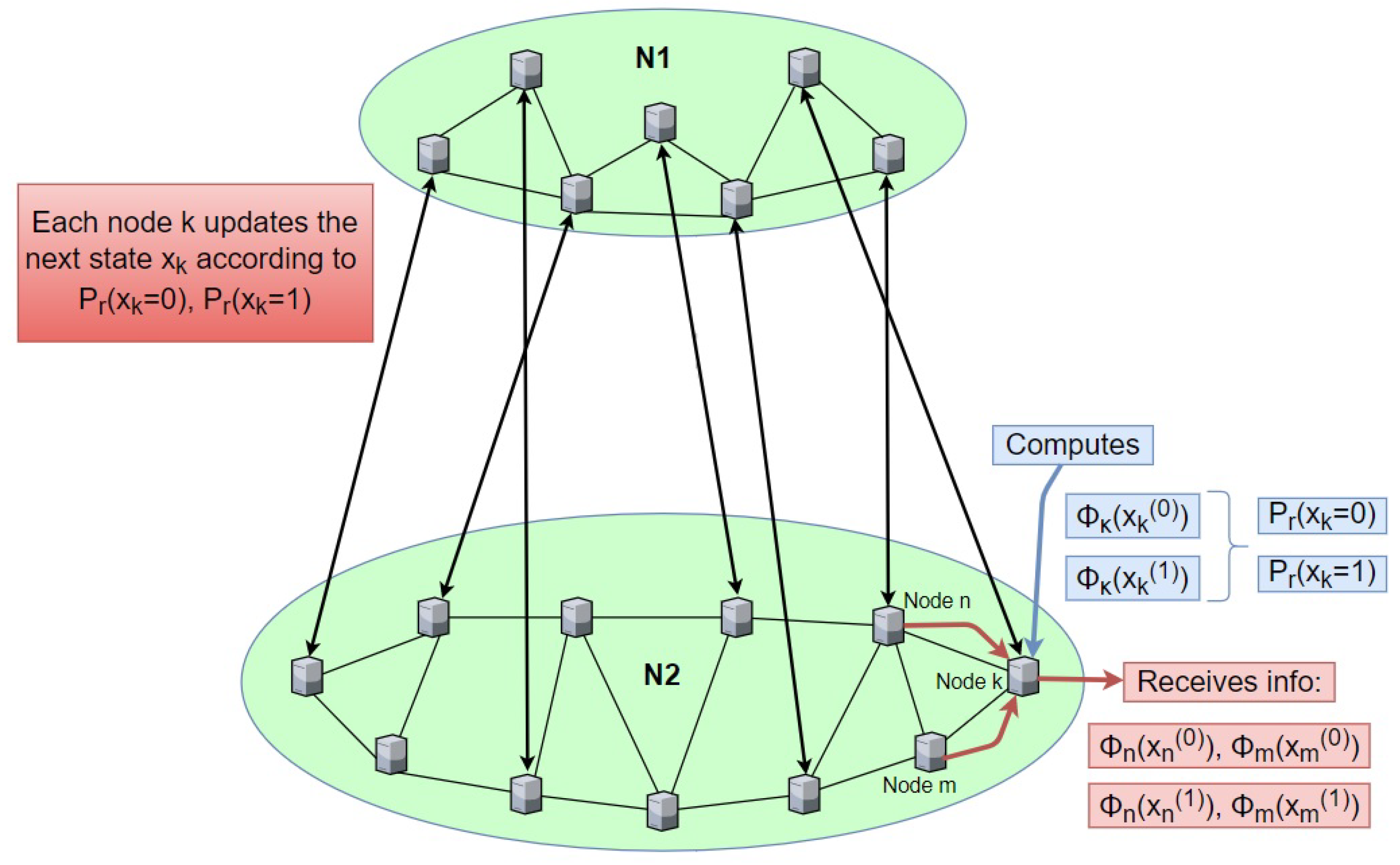
We consider a malware propagative complex communication networks (CCN) with N nodes. In our case, the considered CCN will be a two-layer network, such as the one shown in Figure 1. The term malware propagative denotes that wherever a legitimate node is infected, it can further infect with malware other non-infected legitimate nodes. We study the macroscopic behavior of the system, in which nodes may become infected, then recover to the susceptible state, and become re-infected at a later time instant. This behavior is effectively described by an SIS infection paradigm.

Assume a finite set $S,\left|S\right|=N$, with elements $s\in S$ corresponding to the nodes of the network. We define the phase space $\mathsf{\Lambda }$ as the set of possible states of each $s\in S$. We define a random field on S, the collection $X=\{X_s,\forall s\in S\}$ of random variables with values in $\mathsf{\Lambda }$. A configuration $\mathbf{x}=\{x_s,\forall s\in S,x_s\in \mathsf{\Lambda }\}$ corresponds to one of all possible states of the nodes. The employed MRF framework abstracts connectivity and local interactions through the neighborhood system of each node’s set of neighbors. A neighborhood system on S is defined as a family $\mathcal{N}={\left\{{\mathcal{N}}_s\right\}}_{s\in S}$ of subsets ${\mathcal{N}}_s\subset S$, such that for every $s\in S$, $s\ne {\mathcal{N}}_s$ and $r\in {\mathcal{N}}_s$ if and only if $s\in {\mathcal{N}}_r$. ${\mathcal{N}}_s$ is called the neighborhood of node s. The random field X is called a Markov Random Field (MRF) with respect to $\mathcal{N}$ if for every node $s\in S$,

$$\mathbb{P}(X_s=x_s\mid X_r=x_r,r\ne s)=\mathbb{P}(X_s=x_s\mid X_r=x_r,r\in {\mathcal{N}}_s).$$

(3)

Direct interactions between infected and sensitive nodes are recorded, covering cases where malware infections spread in a localized way that depends on the one-hop communications [43]. However, we can adapt the neighborhood system definition by appropriately defining a new neighborhood system where the nodes involved are direct neighbors (in the overlay topology). The MRF framework achieves macroscopic evolution of the system through point-to-point interactions between adjacent nodes.

For an appropriate MRF modeling of an SIS malware propagation epidemic, we select for each node k a pairwise (depending on neighboring interactions) potential function of the form:

$${\mathsf{\Phi }}_{\kappa }\left(x\right)={\mathsf{\Phi }}_{\kappa }\left(x_{\kappa }\right)=-D\sum _r{\sigma }_{\kappa }{\sigma }_r,\forall r\in N_{\kappa },D>0,$$

(4)

for each pair of neighboring nodes $\kappa ,r\in S$. Function ${\sigma }_{\kappa }$ is a bijective function of $x_i$, $x_i$ being the node state with 0 denoting a susceptible node, 1 denoting an infected one and $\mathbf{x}$ being the vector of all node states denoting the overall system state. Parameter D is a constant scaling factor that can be used to change the sensitivity of the MRF model. The exact definition of the node-specific function $\sigma (·)$ can slightly affect the sensitivity of the model but not the observed behavior. The exact potential function essentially captures the pairwise interactions between network nodes and quantifies the outcome of such interactions, depending on the individual node states, e.g., interactions between infected–susceptible nodes, infected–infected, and susceptible–susceptible. All contributions are aggregated and reflected in the total “energy” value of the system. The goal is to bring the system to a state with the least possible energy, the latter being symbolized by the potential function divided by temperature. Simulated annealing (SA) can be combined with Gibbs sequential sampling to analyze the evolution of the cumulative state of the system. An RF X is called a Gibbs Random Field (GRF) if it satisfies:

$$\mathbb{P}\left(X=\mathbf{x}\right)=\frac{1}{Z}{e}^{-\frac{U\left(\mathbf{x}\right)}{T}},$$

(5)

where $Z:={\sum }_{\mathbf{x}\in {\mathsf{\Lambda }}^n}{e}^{-\frac{U\left(\mathbf{x}\right)}{T}}$ is called the partition function and T is called the temperature of the system. $U\left(\mathbf{x}\right)$ is the general potential function mentioned above. It is not unique.

The approach works as follows. In each iteration, each node is visited once according to a specific visiting scheme, and the status of each site is updated according to its neighboring situations, depending on its possible operation. The process is repeated for a number of scans s until the system converges to its steady state. Before this iterative process, a temperature $T(·)=T\left(s\right)$ and the maximum number of scans s are selected. SA requires a gradual reduction in temperature as the simulation progresses, so that the system initially wanders to a wide area of the search space that contains good candidate solutions. It then drifts to low-energy areas and finally downhill according to the steepest heuristic descent. For each node, a binary decision is made as to whether its status will remain the same for the next scan or change. For every possible value of each state $l\in {\mathsf{\Lambda }}_{\kappa }$, where ${\mathsf{\Lambda }}_{\kappa }$ is the phase space of the node $\kappa$, the potential function for each position $\kappa$, ${\mathsf{\Phi }}_{\kappa }\left(x_k^l\right)={\mathsf{\Phi }}_{\kappa }\left(x_{\kappa }\right)=l,x_{\kappa }^{\prime }:{\kappa }^{\prime }\in N_{\kappa }$, depends only on the state of node k and the states of all neighboring sites ${\kappa }^{\prime }\in N_{\kappa }$. The decision for the next state of each node can be made according to the following probability:

$$Pr(x_k=\ell )=\frac{e^{-\frac{{\mathsf{\Phi }}_k\left(x_k^{(\ell )}\right)}{T\left(n\right)}}}{{\displaystyle \sum _{{\ell }^{\prime }\in {\mathsf{\Lambda }}_k}}{e}^{-\frac{{\mathsf{\Phi }}_k\left(x_k^{\left({\ell }^{\prime }\right)}\right)}{T\left(n\right)}}}.$$

(6)

Thus, with the above probability, the next state of node k will be ℓ. Given that ${\mathsf{\Lambda }}_k=\{1,0\}$ in our case, corresponding to infected and non-infected (susceptible) states, the above can be written in a simpler general form:

$$Pr(x_k=\ell )=\frac{1}{1+e^{-\frac{{\mathsf{\Phi }}_k\left(x_k^{\left({\ell }^{\prime }\right)}\right)-{\mathsf{\Phi }}_k\left(x_k^{(\ell )}\right)}{T\left(n\right)}}},$$

(7)

where $\ell ,{\ell }^{\prime }\in \{0,1\}$ and $\ell \ne {\ell }^{\prime }$.

Taking into account the values of the phases in the defined phase space, we have chosen the following potential function expressions:

$$\begin{array}{c}\hfill {\mathsf{\Phi }}_k(x_k^{\left(0\right)})=-J\sum _{k^{\prime }\in {\mathcal{N}}_k}{\sigma }_k{\sigma }_{k^{\prime }}=-J\sum _{k^{\prime }\in {\mathcal{N}}_k}{x}_k{x}_{k^{\prime }}=0,\end{array}$$

(8)

$$\begin{array}{c}\hfill {\mathsf{\Phi }}_k(x_k^{\left(1\right)})=-J\sum _{k^{\prime }\in {\mathcal{N}}_k}{\sigma }_k{\sigma }_{k^{\prime }}=-J\sum _{k^{\prime }\in {\mathcal{N}}_k}{x}_k{x}_{k^{\prime }}=-J\sum _{k^{\prime }\in {\mathcal{N}}_k}{x}_{k^{\prime }},\end{array}$$

(9)

which yield the following expressions for the node state probabilities:

$$\begin{array}{ccc}\hfill Pr(x_k=1)& =& \frac{1}{1+e^{-J\frac{{\displaystyle \sum _{k^{\prime }\in {\mathcal{N}}_k}}{x}_{k^{\prime }}}{T\left(n\right)}}},\hfill \end{array}$$

(10)

$$\begin{array}{ccc}\hfill Pr(x_k=0)& =& 1-Pr(x_k=1)=\frac{1}{1+e^{J\frac{{\displaystyle \sum _{k^{\prime }\in {\mathcal{N}}_k}}{x}_{k^{\prime }}}{T\left(n\right)}}}.\hfill \end{array}$$

(11)

The annealing pattern is chosen as $T\left(s\right)=\frac{c_0}{logn}$, where $c_0$ is a constant $(c_0=1000)$ that affects the convergence and accuracy of the model. Higher values $J/c_0$ correspond to more vulnerable topologies where malware spreads more easily, while lower values correspond to more powerful ones. The maximum number of scans is selected as s = 2000. Such a number ensures that the sampling process converges to the steady-state system with a high probability, which is verified by ensuring that the system state remains unchanged for a number of consecutive scans. The selected parameter ensures this for all scenarios, as they proved to be sufficient even for smaller values s, e.g., s = 1000 or 1500 scans. All the results that will be presented for each type of network have been calculated on average in 25 different scenarios.

In terms of attacks, we focus on non-smart (random) malware attacks, starting with a single intruder (infected), where the infected node is unable to use any side information to help spread the malware. The intruder and the infected nodes communicate only through point-to-point contacts, and susceptible nodes are infected with the same probability of infection when they come in contact with infected/malicious nodes. Consequently, such non-smart attacks can be considered as “blind” (random) attacks against vulnerable one-hop neighbors. Random attack vulnerability analysis is just one of the many applications that the MRF framework can host.

At this point, we need to note an important aspect of the MRF framework presented above. Malware propagation may have some preferential directions, e.g., an Android-based malware will follow the “direction” of other Android devices but not the direction of iOS devices. MRFs can be applied equally well in directed graphs [63]. An MRF is essentially defined on a neighborhood system, namely the set of all neighborhoods formed by the nodes of the graph. In case of a directed process, the underlying graph will be directed, but each node will be equally fit to define its neighborhood, on which it will be possible to perform the distributed Gibbs sampling with simulated annealing. The rest of the model can remain unchanged.

4. Epidemics Spreading in Multi-Layer Complex Networks via Markov Random Fields

In this section, we provide the results obtained for each separate scenario via the use of the MRF malware modeling framework.

4.1. Analysis of Random Markov Fields on Spreading Malware

We considered a Markov Random Field (MRF)-based framework for modeling the macroscopic behavior of a multi-layer CCN under random attack, where malicious threats propagate through direct interactions and follow the Susceptible–Infected–Susceptible infection paradigm. We studied the behavior of two-layer systems for various topological and malware-related parameters with respect to the general random attacks considered. We demonstrate the effectiveness of the MRF framework in capturing the evolution of SIS malware propagation and use it to assess the robustness of synthetic CCNs with respect to the involved parameters.

We focus on the cumulative number of infected nodes and not on the state of each node in particular. The MRF framework abstracts connectivity and local interactions through the neighborhood system, focusing on the macroscopic evolution of the system through point-to-point interactions between adjacent nodes. Direct interactions between infected and sensitive nodes are recorded, covering cases where malware infections spread locally similarly to [2].

For malware propagation, $L=0,1$ is the phase space, where ‘1’ corresponds to an infected state and ‘0’ corresponds to the non-infected (susceptible) state. We focus on the interactions between neighboring S–I pairs of nodes. Such pairs drive the evolution of malware propagation. The dynamics of malware depend mainly on interactions between attacking nodes and sensitive users [25,43,44,64]. Thus, in relation to defining an appropriate possible operation for an MRF malware, a pairwise potential is employed. Singleton terms could have also been included, representing the contribution of the nodes themselves to the spread of malware. In such cases, where a node suddenly changes its status from vulnerable to infected and starts spreading malware, various types of malware could be represented, e.g., trojan horse, trapdoors, etc. [65].

With respect to attacks, we start from a single attacker, which is constantly infected. The attacker and infected nodes only have point-to-point contacts with susceptible nodes, which are homogeneously infected, i.e., they become infected with the same infection probability when in contact with infected/attack nodes. Here, we focus on these types of attacks in order to demonstrate how the MRF can be used for network robustness analysis and reveal salient features of the framework.

4.2. System Setup

We consider two-layer complex topologies, as shown in Figure 1; also, we consider that each layer may be of different type, i.e., random, small-world, etc. To examine each aspect of the day-to-day networks represented by these combinations, we set the number of nodes in the first network equal to 100, 250, and 500 nodes. Meanwhile, for the corresponding topology that is connected, we defined the nodes equal to 100, 250, 500, 750 and 1000. That is, keeping the number of nodes of the first topology constant, we modified the number of nodes of the second. To cover a wide range, 25 scenarios of each correspondence between the node numbers were repeated, and finally, the average of the infected nodes of our final network was obtained.

To better account for the interaction of the two topologies and the resulting infected nodes, we created vertical links between these two topologies. These vertical connections must also increase, as our network grows, in order to be able to properly and effectively relate the connection and interaction of the two network topologies. Therefore, we set them to equal to the number of nodes in the first topology, i.e., 100, 250 and 500.

In order to determine the vertical connections between the two considered topologies, we select a pair of nodes, i.e., one node from the first topology and one from the second at random. This will also be a link between the topologies. We repeat the same procedure for another random pair of nodes, after first making the appropriate check for whether this pair has been used before. This way, we avoid “losing” some vertical connections by randomly selecting the same node pairs.

4.3. Considered Topologies and Scenarios

4.3.1. Random Geometric Graph and Scale-Free

As the first combination of considered topologies, the Random Geometric Graph (RGG) with a scale-free (SF) topology is presented. This corresponds to a possible application where users use their mobile phones to communicate directly and in parallel access different social networks at the same time. The RGG topology corresponds to the direct connections between mobile phones, i.e., connections at the physical layer, while the SF topology corresponds to the interfaces that users have with each other in each social network (cyber layer). Figure 2 shows the results for different sizes of the single topology and for varying numbers of nodes of the second level topology. As expected, the larger the network, i.e., the denser it becomes, the higher the average number of infected nodes in the network. Another observation that stands out is that as the network density increases, the number of infected nodes increases slightly faster than linearly (comparing the results between curves corresponding to N_1 = 100, N_1 = 250 and N_1 = 500).

4.3.2. Random Graph and Random Graph

A second combination of topologies we consider is that of a Random Graph (RG) with another Random Graph (RG), while each topology has different topological parameters. In this case, one topology could correspond to a peer-to-peer file sharing network, while the other could correspond to random users coexisting on the Internet and communicating with each other. Figure 3 shows the results for different sizes of the single topology and for varying numbers of nodes of the second-level topology. As in the previous figure, we obtain similar results regarding the expected number of infected nodes and the network density. However, compared to the last observation in the previous scenario, here, it seems that in terms of the number of N_1, the increase in the average number of infected nodes is closer to having a linear scale.

4.4. Random Graph and Small-World

As a third combination, a Random Graph (RG) topology combined with a Small-World (SW) topology was chosen. The union of these two topologies may correspond to an application where users use their mobile phones to connect to a peer-to-peer file sharing network. In this network, the Random Graph (RG) topology corresponds to the direct connections between mobile phones (physical), while the Small-World (SW) topology corresponds to a social network that develops and has this structure (cyber layer). Figure 4 shows the corresponding results. As we observe the resulting figure, we realize that the larger the network, i.e., the denser it becomes, the greater the average number of infected nodes in the network. The only difference one may notice is that on average, the number of infected nodes in this topology is a bit less than the previous one (RG-RG).

4.5. Small-World and Scale-Free

A fourth combination of complex topologies was chosen to form a potential cyber-physical system consisting of a Small-World (SW) overlaying a Scale-Free (SF) topology. The SW topology might correspond to a growing social network, while the SF topology could correspond to the interfaces that users have with each other in the social network. Figure 5 presents corresponding results to the previous schemes. That is, the number of spoke nodes directly depends on how much the network created by these two topologies grows and becomes dense.

4.6. Regular and Random Graph

The fifth combination we considered was a Regular (REG) topology combined with a Random Graph (RG) topology. Regular topology (REG) can usually correspond to some physical grid-type topology, e.g., sensor network, while Random Graph (RG) topology can correspond to random users coexisting on the Internet and communicating with each other in their communication with the display or even otherwise using the physical topology. In a grid topology, such as REG, all nodes are interconnected, i.e., we have a fully interconnected topology. This is the most expensive but also the most secure topology model, as a message goes only to the correct recipient; while nodes become infected and malfunction, they do not affect the rest of the network nodes. The shape Figure 6 also shows similar results to the previous graphs. Of course, in this particular example, we notice that with regard to the scaling with respect to the different values of N_1, here, the observation of the first scenario (RGG - SF) is valid; that is, as the density of the network increases, the number of infected nodes increases slightly faster than linearly.

4.7. Regular and Scale-Free

The last combination of topologies was again considered a Regular (REG) topology for the physical system combined with a Scale-Free (SF) for the cyber portion of the network. The Regular (REG) topology corresponds, as in the previous example, to some physical network type topology, e.g., sensor network, while the Scale-Free (SF) topology can be considered as an alternative to the RG topology considered in the previous scenario, mirroring the interfaces that users have with each other in the social network. Figure 7 shows the corresponding results with the previous graphs. In this particular example, we notice again that regarding the scaling with respect to the different values of N_1, here again, the observation of the first scenario (RGG - SF) applies. Thus, we conclude that as the network density increases, the number of infected nodes increases slightly faster than linearly that when we choose an RG topology.

5. Discussion

In this section, we perform a cumulative comparison across the considered scenarios for the purpose of obtaining useful observations and insights. We are mostly interested in observations and their reasoning regarding the structural properties and behavioral features expressed by different types of considered topologies.

The following figures present cumulative results for all considered scenarios, aiming towards comparing among the different combinations of the considered complex topologies and the extraction of longer-term useful observations. Figure 8 presents the cumulative results when N_1 = 100 nodes, Figure 9 presents the cumulative results when N_1 = 250 nodes, and Figure 10 presents the cumulative results when N_1 = 500 nodes. These three figures allow comparing the behavior of the considered scenarios and topologies with respect to the size of the first topology. The first interesting outcome is that a quite similar behavior is exhibited among the different scenarios as the first network becomes larger (and denser). This is due to the fact that some of the topologies share some common features, e.g., SW with SF, etc. The less vulnerable combination is that of RGG-SF, while the most vulnerable one being the RG-RG. The performance of the rest of the schemes performing in between these two extremes remains the same for all three values of the size of the first network. This is due to the fact that the epidemic behavior depends more on the structural properties of the corresponding topologies rather than on the exact size (density of the network). Of course, as can be observed by the three figures, there is more prominent segregation of the relative performance as the topology of the first network becomes larger. The topology determines the neighboring relations and thus defines terminally the allowed interactions and hence the allowed diffusion paths in the network. In any case, the structural feature seems to have a stronger effect than the size of the topology.

Then, Figure 11, Figure 12, Figure 13, Figure 14 and Figure 15 present similar cumulative results for the number of infected nodes when the second topology has N_2 = 100, 250, 500, 750 and 1000 nodes, respectively. Such figures allow comparing the behavior of the considered scenarios–topologies as well, this time with reference to the second topology. A similar interesting outcome, as in the previous case, is that a quite similar behavior is exhibited among the different scenarios in each figure, as the second network becomes larger (and denser). However, here, the relative ordering of the behavior of each combination changes. The more robust combination is that of RG-RG, while the most vulnerable one is the RGG-SF. The relative ordering of the performance of the schemes in between remains the same for all the considered sizes of the second topology. The reason for the repeating relative ordering is again the fact that the epidemic behavior depends more on the structural properties of the corresponding topologies rather than on the exact size (density of the network). The segregation of the relative ordering is again due to the second topology becoming more dense and thus producing more epidemic events in the corresponding scenarios. The modification in the relative ordering compared to the previous set of results is due to the nature of the type of each employed topology as second topology in the two-layer combination. Differences in the density of such topologies lead to different relative orderings. In any case, the structural feature prevails overall, having a stronger effect than the size of the topology.

Through the above analysis for random attacks, it can be concluded that overall, and with gravity of importance on the factors of structural topology, the combination RGG-SF is more vulnerable. Second in order of vulnerability follows the combination of the SW-SF, which is followed by REG-SF and RG-SW. Finally, the combinations REG-RG and RG-RG are observed to be the most reliable.

More specifically, in the RGG-SF combination, it is observed that the spread of malware on the network is more intense, resulting in more network nodes being infected as the density of the topology increases. In the combinations SW-SF and REG-SF, similar results are observed, as the spread of malware in networks such as a developing social network or some natural grid-type topology (e.g., sensor network), when malware comes in contact with the interfaces that users have with each other in the social network is less harmful and the network is quite reliable. The RG-SW combination, representing, e.g., a network where users connect with their mobile phones to a peer-to-peer network, is equally vulnerable and reliable. The possible shortcuts in the topology introduced by the SW part of the network reduce the robustness potentials of the RG part, which if independent would exhibit very good robustness performance [2].

The most reliable and least vulnerable networks according to the research results are those of the combinations REG-RG and RG-RG, respectively, i.e., some natural grid-type topology, e.g., sensor network, over which users may access a social or other type of information exchange network. This is due to the fact that the grid-like part of the topology ensures local interactions, while the random part of the topology provides the necessary randomization with respect to the contacts. This means that even though there might be intense local epidemic incidents, these will propagate randomly, and thus, they will not necessary hit on key nodes, eventually diminishing the potential effect of strong epidemics.

It is very important to note that as the final network density increases, in most of the studied topologies, the percentage of infected nodes reduces relevantly, i.e., the increase of the number of expected infected nodes increases linearly or mostly sub-linearly. Thus, on larger networks, malware is less harmful and can be restricted more easily. Even if we set the initial number of infected nodes equal to 10, we observe that the final number of infected nodes does not differ much from the final number of infected nodes when we set the initial number of infected nodes equal to 1. This phenomenon was observed and investigated in all topologies analyzed, of all sizes. Our results show that the final number of infected nodes is eventually more due to the topological features of the network topologies themselves and their density rather than due to the initial number of malicious nodes that may begin the epidemic.

6. Conclusions and Future Research

6.1. Summary

In this work, we studied the modeling of malware in multi-layer network topologies and more specifically in two-layer topologies, representing possible cyber-physical systems. We observed and recorded the propagation of malware, starting in each case from a random node of the network, in the two-layer network that we set each time. The considered two-layer topologies combine different types of complex networks, which represent potential networks emerging in our daily lives and more specifically topologies emerging as cyber-physical systems. A Markov Random Field (MRF)-based framework was used to model the propagation of random malware throughout the systems under consideration. We study such systems macroscopically, in the sense that over a long period of time, vulnerable nodes can be infected and then fully recover only to be infected again by another malware. Thus, we considered the SIS paradigm for the MRF-based propagation model. By combining Gibbs sampling with simulated annealing, we obtained the long-term statistics of the propagation of such malware in the considered topologies through the expected number of infected nodes in each scenario. The main results are that networks with denser topologies ultimately offer greater flexibility in handling random malware regardless of its type. Regarding vulnerability, the most reliable and least vulnerable networks were observed in the combinations of REG-RG and RG-RG topologies, that is, the combination of a physical mesh-type topology or a topology that could correspond to a peer-to-peer file sharing network, in combination with a topology that corresponds to the random users that coexist on the Internet and communicate with each other.

6.2. Future Work

Multiple directions have been identified for future work. An interesting one was mentioned before, involving the study of the model and of the propagation in directed topologies, modeling “preferential” malware. A second direction for future work is the analysis and extension to systems with more network layers (third and fourth layers), thus listing networks that we use in our daily life, even up to the semantic layer. Finally, a more practical direction for extension would be to study the results of this work in real cyber-physical systems for cross-validation of the results.