Management of Coastline Variability in an Endangered Island Environment: The Case of Noirmoutier Island (France)

Abstract

This article presents a diachronic study of evolution along the coastline of Noirmoutier Island in France, a sandy shore particularly susceptible to erosion and submersion risks, which are exacerbated by climate change due to two-thirds of its territory being below sea level. The study is based on an analysis of aerial images covering a period of 72 years, divided into five distinct periods: 1950–1974, 1974–1992, 1992–2000, 2000–2010, and 2010–2022. The methodology used combines two complementary approaches: the Digital Shoreline Analysis System (DSAS) for taking linear measurements of the erosion and accretion that have taken place along various shorelines, and the surface method to evaluate the amount of surface lost or gained between different shorelines while calculating the uncertainties associated with the obtained results. The overall trend observed between 1950 and 2022 indicates that the Noirmoutier coastline studied has gained surface area (81 hectares) at an average rate of +0.57 ± 0.06 m per year. The article then presents an application of the method developed by Durand and Heurtefeux in 2006 to estimate the future position of the shoreline. A map of the local area is also provided, identifying the areas susceptible to coastal erosion by 2052 and by 2122, in accordance with the provisions of the Climate and Resilience Law adopted in France on 22 August 2021. The results reveal that there are many sources of uncertainty in predicting the future evolution of the shoreline using this methodology. Therefore, it is crucial to consider these uncertainties when planning future coastal management actions and adopting appropriate adaptation methods to counteract unforeseen developments.

1. Introduction

Coasts are highly esteemed but vulnerable and changing environments that are subject to natural processes such as currents, waves, tides, storms, and anthropic processes such as artificialisation, the installation of structures, preventive and curative management operations, and beach replenishment, all of which have been widely studied over a long period of time [1]. The risk is generated by the intersection of these processes, along with the presence of coastal hazards such as erosion and marine submersion [2]. The geographic co-occurrence of these hazards and the issues affecting the coastal strip are the reasons why coastal risk has increased since the 1960s [3]. The heightened vulnerability of the coastline due to both human and non-human factors is also at the centre of a huge debate, and the issue has now been generally taken on board by the scientific community and public authorities [4].

In the wake of Storm Xynthia on 28 February 2010, which had an enormous impact on the central area of France’s Atlantic coast, and in respect of climate change forecasts [5], it is apparent that we must improve our overall understanding of the phenomena that affect the sea–land interface. This necessity underscores the importance of continuously monitoring and detecting spatio-temporal changes in shorelines to keep track of the changes and understand the vulnerability and risks associated with natural disasters [6]. Analysing coastal development has become an indispensable pre-requisite for coastal management due to the need to reduce risks [7]. To do this, it is essential to understand how the coastline has evolved according to the associated temporal scales and to have a reliable tool to enumerate, estimate, and predict the shoreline movement landward or seaward [8]. A growing number of studies have highlighted the effects of the climate change processes, both recognised and assumed, associated with each spatio-temporal scale, with the probable overall consequence, as observed both now and in the past, of an increase in coastal variability [9,10,11].

Confronted with these challenges, the Climate and Resilience Law, adopted in France on 22 August 2021, under the number 2021-1104, has introduced a mechanism to strengthen the resilience of coastal areas. In particular, the mechanism includes the establishment of maps indicating risks associated with coastline recession in the short and long term and providing tools with which local authorities can combat or adapt to coastal erosion and predict how it will develop.

The aim of this article is to improve knowledge and understanding of the evolution of the Noirmoutier coastline (France), both current and historical, and evaluate potential developments over 30 and 100 years in terms of climate change and increasing pressure on the land. The work is essential to provide decision-makers and local authorities with reliable data to inform the implementation of coastal management and adaptation strategies in line with the requirements of the Climate and Resilience Law and to consider the specific island characteristics of the Noirmoutier coast.

2. Characterisation of the Study Area

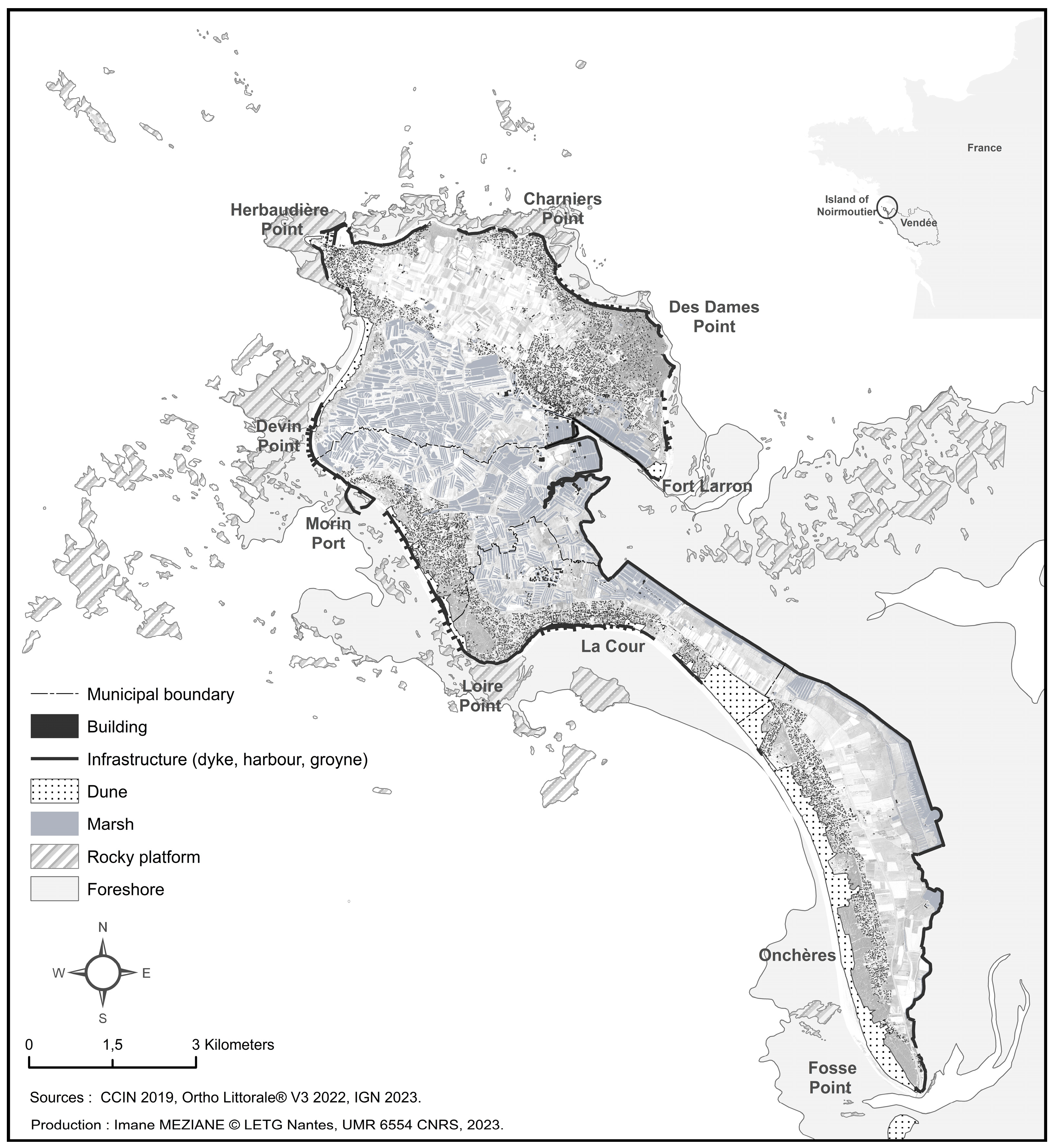
2.1. Outline of the Study Area

The island of Noirmoutier is an insular territory located on the Atlantic coast of France, integrated into the department of Vendée. It is 18 km in length and varies in width from 500 m to 6 km, occupying a total area of 49 km². Two-thirds of the island of Noirmoutier is below the average level of the open sea at high tide [12]. The northern part of the island comprises a rocky plateau, with the western side having a series of dune ridges stretching northwest to southeast (Figure 1). The low-lying areas behind this ridge have gradually been reclaimed. The eastern side of the island is protected by a system of dykes. Urban development has taken place mainly on the northern plateau and dune ridges (Figure 1).

The area is a semi-diurnal macrotidal type, with a mean tidal range of 3.4 m [13]. In terms of hydrodynamic characteristics, westerly winds have been the most frequent between 1979 and 2022, at 10.12% [14]. Overall, SW to WSW winds dominate (40%). Winds from the NE and ENE are secondary (15%). In terms of wave climate, the most frequent waves predominantly originate from the west (73%). The second most frequent is WSW, at around 16%. The highest significant wave heights reach 1.84 m on average, with the maximum being 10.9 m [14].

In terms of coastal protection structures, several installations have been installed to protect the shoreline. The table below (

Table 1. Summary of coastal protection structures on the island of Noirmoutier [15].

Category	Class	Type	Number	Cumulative Length (km)
Protective structures	Structure replacing the shoreline	Coastal dyke	18	21.9
		Retaining wall	11	1.7
		Stone revetment	35	8.9
	Erosion control structure	Breakwater	2	0.3
		Groyne	74	4
Other coastal developments	Access	Entrance, path, submersible causeway, etc.	1	3.8
		Slipway	7	0.3
	Constructions	Building, blockhouse, fortification, etc.	2	0.1
		Individual protection	16	2.4
	Port and navigation infrastructure	Jetty	6	2.3
	Miscellaneous	Other or unidentified	17	1.3
Total			189	47

) gives a summary of the main installations.

The Noirmoutier coast has been the subject of various projects to divide it into hydro-sediment cells [16,17]. As a result of these studies and the demarcation of the cells by fixed landmarks (rocky headlands, jetties, dykes, and slipways) and mobile landmarks (the reversal point of the longshore drift), nine littoral cells were identified along the coastline, as shown in Figure 2 (the term “littoral cells” is used, according to Carter [18], Bray et al. [19], Frihy et al. [20] and Anfuso et al. [21]). The eastern side of the island forms a littoral cell (LC) subdivided into three sections running from south to north (A, B, and C), corresponding to the same sedimentary units as defined by DHI [16]. The western side represents littoral cell 2, divided into six sections running from north to south (A, B, C, D, E, and F), following the divisions established by Parcineau [17], with the exception of LC2-E, which has been divided into two distinct littoral cells, forming a mobile boundary at the point of inversion of littoral drift.

2.2. Regulatory Context

French legislation relating to the policy on prevention of coastal risks is based on a number of framework laws introduced to ensure the coastal areas are protected and forestall risks linked to erosion, sea level rise, and extreme weather events. The Coastal Law of 3 January 1986 on developing, protecting, and enhancing the coastline is the mainstay of this legislation. It is an essential pillar of French law governing urbanisation, prohibiting any construction within a 100-metre strip, and is part of a strategy designed to balance development of the coastal area with the preservation of ecosystems that are under threat, responding therefore to both natural exigencies and those linked to the increasing pressure of human activity. Other legislation has subsequently been brought in to reinforce this protection policy, including the Barnier Act of 1995, which introduced Risk Prevention Plans (PPR) to define areas exposed to natural threats. The Grenelle II Law of 2010 likewise brought in environmental provisions to reinforce protection by introducing climate change measures. The more recent Climate and Resilience Law, enacted on 22 August 2021, has brought about significant changes by consolidating coastal risk prevention measures and combining them with measures to ensure shoreline retreat is incorporated into urban planning by producing local maps of the shoreline showing predicted erosion within 30 and 100 years.

3. Methodology

3.1. Data Presentation

Shoreline evolution trends were calculated from shoreline positions extracted from aerial images covering the 1950–2022 period.

Table 2. Inventory of aerial images.

Date	Type of Data	Source	Scale
1950	BD ORTHO® HISTORIY	GEOPAL (IGN)	1/25,000
1974	Aerial photo	CCIN (IGN)	1/30,000
1992	Aerial photo	CCIN (IGN)	1/30,000
2000	Ortho Littorale®	Géolittoral (IGN)	1/25,000
2006	BD ORTHO® V2	CCIN (IGN)	1/25,000
2010	BD ORTHO® V2	CCIN (IGN)	1/25,000
2016	BD ORTHO®	CCIN (GEOVENDEE)	1/25,000
2020	Ortho Littorale® V3	CEREMA (GEOFIT)	1/25,000
2022	Ortho Littorale® V3	CCIN (Department)	1/25,000

gives a summary of the dataset.

3.2. Choice of Shoreline Position Marker

The shoreline is defined as the physical interface between land and sea, where the action of marine processes on the continental zone ends [22]. There are many different markers identifiable from aerial photographs that can be used to determine the precise position of a shoreline, including hydrodynamic, morphological, and biological indicators [22,23].

The choice of marker fell on the extent of dune vegetation, as this is the most conclusive indicator of how sandy coastlines have evolved in the medium and long term [24]. It is also quite easy to see on low-resolution aerial photographs [25]. In cases where no dune vegetation was visible, the dune toe was used as a marker.

3.3. Methodology for Calculating the Historical Evolution of the Shoreline

Various methods can be used for diachronic analyses of the shoreline [22,23,26,27,28,29,30,31,32,33]. The interpretation of aerial photographs, analysis of maps (historical, topographical, and hydrographic), study of satellite images, field surveys, and interviews with local residents all constitute valuable sources of information for studying the shoreline [34]. These data are subsequently compared using either transect-based analysis or area-based analysis methods. The former is based on the measurement of the distance between each shoreline at set points along transects [35], while the latter calculates the total surface area to evaluate the extent of loss by erosion, or gain by accretion, between two shorelines over a given period.

3.3.1. Kinematic Analysis of the Shoreline by Transects

The stability of the shoreline was analysed and estimated using extension 5.1 of the Digital Shoreline Analysis System (DSAS), provided by the USGS (United States Geological Survey) and operated by the Esri ArcGis 10.8 software [36]. The DSAS method involves marking a baseline parallel to the position of the shoreline, either on the onshore or offshore side. In this case, the line corresponds to the onshore boundary of a 300 m² buffer zone around the digitised shorelines.

The line was then used as a starting point to draw equally spaced perpendicular transects every 20 m along the coast [37,38,39], this distance being the best suited to the small beaches in the study area [40]. Finally, the rate of shoreline evolution was calculated along each transect according to the End Point Rate (EPR) method, which consists of dividing the distance of net movement along the shoreline (NSM) calculated on the transect between the oldest and the most recent shorelines by the number of years separating them [41,42,43].

3.3.2. Surface Analysis of the Shoreline Evolution

The surface evolution of the shoreline was analysed using spatial units known as ‘boxes’, inspired by the work of Debaine and Robin [13], Juigner et al. [44], Juigner and Robin [45], Kerguillec et al. [46] and Robin et al. [47]. Boxes were created between the two shorelines—the historic one and the recent one—for each period of the study, using transects spaced 20 m apart. Boxes were created where the transects intersected with the coastline, retaining only the surface area between the two shorelines. Each box was bounded by four lines: two transects and two longitudinal lines representing the former and recent shorelines. The depth of each box varied depending on the distance between the two shorelines. The surface analysis was accomplished by calculating the area of each box for each littoral cell using ArcGIS software. This involved grouping the boxes in each littoral cell and calculating the total area gained or lost for each group of boxes in square metres.

3.3.3. Cartographic Representation of the Historic Shoreline Evolution

Evolutionary trends, calculated every 20 m along the sandy coastline of the study area, were represented as uniform boxes of 20 × 250 m. The rates of evolution were discretised into ten distinct classes, each allocated a different colour to facilitate clear, concise visual analysis of the variations along the coast (Figure 3). Note that these boxes are different from those used to estimate surface uncertainty. Each box was bounded by four lines: two transects and two longitudinal lines, offshore and onshore.

Erosion is represented by shades of yellow and orange, and accretion by shades of green and blue. The boundary between the erosion and accretion trends appears as a grey band, representing a margin of error of ±0.25 m/year. This value was obtained by calculating the mean value of the errors for each period studied. Longitudinal protection structures are also identified on the map in white, but they are excluded from calculations of evolution rate.

3.3.4. Estimation of Error

Several sources of error affect the accuracy of positioning the shoreline and consequently the results of analyses [23,27,28,30,33,48]. Three were measured in this study [38,47,49]. One is the pixel size of the aerial images; another is the accuracy of the orthorectification or georeferencing process, which uses root mean square error (RMSE); and finally, the digitisation error refers to the average distance between the digitisation of two shorelines from the same aerial image by different operators. The overall positioning error for each stretch of coast (

Table 3. Summary of linear errors on the digitised shorelines.

$\mathbf{A}.\mathbf{Calculation}\mathbf{of}\mathbf{overall}\mathbf{shoreline}\mathbf{position}\mathbf{error}{\mathbf{E}}_{\mathbf{sp}}$ (m) = (Epixel 2 + Eortho 2 + Edig 2) 0.5
Year	1950	1974	1992	2000	2010	2022
Epixel—Pixel error (m)	0.5	1	0.58	0.5	0.5	0.5
Eortho—Orthorectification error (m)	2.83	2.83	2.83	2.83	2.83	2.83
Edig—Digitisation error (m)	1.68	2.00	1.91	1.60	0.50	0.23
${\mathrm{E}}_{\mathrm{sp}}\text{—}$Overall error (m)	3.33	3.61	3.46	3.29	2.92	2.88
B. Calculation of period error${\mathbf{E}}_{\mathbf{s}\mathbf{p}\mathbf{/}\mathbf{I}}$(m) = (${\mathbf{E}}_{\mathbf{sp}}$ 2 a + ${\mathbf{E}}_{\mathbf{sp}}$ 2 b) 0.5 and E$\mathit{\alpha }$ (m/an) = (${\mathbf{E}}_{\mathbf{s}\mathbf{p}\mathbf{/}\mathbf{I}}$)/I, where a = date a and b = date b
Period (year)	1950–1974	1950–2022	1974–1992	1992–2000	2000–2010	2010–2022
I—Interval (year)	24	72	18	8	10	12
${\mathrm{E}}_{\mathrm{sp}/\mathrm{I}}$—Overall error (m)	4.91	4.40	5.00	4.78	4.40	4.10
$\mathrm{E}\alpha$—Periodic error (m/year)	0.20	0.06	0.28	0.60	0.44	0.34

A) was calculated using the square root of the sum of the squares of each error [30,33,48,49]. The method for producing an annual value for this error between two dates (Table 3B) consists of calculating the square root of the sum of the overall error for each date and dividing it by the period of time that has elapsed between the two dates [30,33,48].

The surface uncertainty for the period (E_sp²,

Table 4. Summary of surface errors.

Littoral Cells (LCs)	1950–1974		1950–2022		1974–1992		1992–2000		2000–2010		2010–2022
	Cl (m)	Esp2 (m2)	Cl (m)	Esp2 (m2)	Cl (m)	Esp2 (m2)	Cl (m)	Esp2 (m2)	Cl (m)	Esp2 (m2)	Cl (m)	Esp2 (m2)
LC1-A	1856	9107	778	3425	1008	5039	868	4147	680	2988	523	2147
LC1-B	2433	11,940	332	1463	1402	7013	302	1442	227	999	151	618
LC1-C	3373	16,557	625	2751	3091	15,457	736	3517	359	1579	325	1335
LC2-A	2796	13,723	643	2832	3870	19,352	802	3832	632	2777	417	1710
LC2-B	701	3440	414	1824	254	1268	255	1217	98	433	136	556
LC2-C	4480	21,990	1523	6707	3268	16,341	914	4363	673	2957	668	2738
LC2-D	643	3157	925	4075	936	4683	1470	7022	887	3898	545	2236
LC2-E	7235	35,510	2938	12,938	5218	26,091	4487	21,430	2429	10,680	2105	8632
LC2-F	3087	15,153	3171	13,964	3170	15,851	3182	15,197	3180	13,980	3256	13,352
Overall coastline studied	26,604	130,577	11,349	49,979	22,218	111,095	13,016	62,167	9164	40,290	8125	33,324

) was calculated by multiplying the overall coastline position error (E_sp, Table 3A) by the length of the coastal stretch (C_l, Table 4) by the littoral cell for each period studied.

3.4. Shoreline Projection Methodology

Several authors have produced overviews of the status of predictive analysis research [50,51,52,53,54,55,56,57,58]. There are various shoreline projection methods that consider the rise in sea level, for example, the Bruun [9], the Durand and Heurtefeux [59], and the Ranasinghe et al. [60] methods. In this study, the projection of the shoreline due to sea level rise was calculated along each transect, spaced 20 m apart. This estimate was based on the following formula, using the Durand and Heurtefeux method [59]:

R = r + [(E21 − E20)/P]

where R = predicted recession at a given time (in metres); r = recession predicted by linear regression (in metres); E21 = projected sea level rise by the given time (in centimetres); E20 = average annual sea level rise in the 20th century (in centimetres), multiplied by the duration of the projection (this value needs to be deducted because it has already been taken into account in the prediction by linear regression); P = slope of the lower beach and the higher part of the upper beach (%).

In this case, the variable “r” was obtained by multiplying the average annual rate (Tx) by the respective duration of each horizon. Tx was determined based on nine historical evolution dates over a long-term period (1950, 1974, 1992, 2000, 2006, 2010, 2016, 2020, 2022) and seven dates over a short-term period (1992, 2000, 2006, 2010, 2016, 2020, 2022) along transects spaced at 20-metre intervals. On each transect, the linear regression rate (LRR) method is employed using the DSAS extension. This method involves fitting a least-squares regression line to all shoreline transect points [36]. The calculation of Tx by the LRR method was compared with that obtained by the EPR method, revealing similarity with correlation coefficients of 0.97 for the 1950–2022 period and 0.98 for the 1992–2022 period.

This annual movement rate was calculated over an observation period equivalent to the projected period [61]. This being a significant historic period, two tests were carried out to assess whether the selected historic period would affect the future position of the shoreline for projection to the target horizon. Another aspect of the tests was to consider two scenarios: the longitudinal structures being retained in the first test and eliminated in the second. This distinction was crucial since it enabled the shoreline projection in the anthropised areas to be evaluated in the absence of structures, leading to consideration of how the shoreline would have evolved in these areas if the current developments had not taken place and there had been no coastal management.

Test 1

The Tx was calculated for a 30-year horizon between 1992 and 2022 and for a 100-year horizon between 1950 and 2022. Data from the 1950s were only used because no data were available going back to the 1920s. For the 30-year horizon, the Tx calculated between 1992 and 2022 was multiplied by 30 to obtain a projection over a 30-year period, starting from the 2022 reference shoreline. Additionally, for the 100-year horizon, the Tx calculated between 1950 and 2022 was multiplied by 70 to project over a 70-year period from the 2052 shoreline (with 70 corresponding to the number of years between 2052 and 2122). The structures were considered to be fixed for this test.

Test 2

Based on previous observed trends at different periods, the historic period used to calculate Tx was between 1950 and 1974. This period was chosen to ensure the rate was truly historic and not influenced by any longitudinal coastal structures that may have been installed since. The Tx calculated for the period between 1950 and 1974 was multiplied by the number of years for the projection. For this test, the projection was 48 years, starting from the 1974 shoreline and arriving at its new position in 2022, in the hypothetical scenario where no coastal management has taken place. This rate was then multiplied by the respective duration of each horizon, i.e., 30 years for the shoreline projected in 2022 and 70 years for the shoreline projected in 2052.

The “E21” variable is the rise in sea level for the given time horizons (30 or 100 years). The value of E21 differs according to which projection is chosen from the five proposed by the IPCC (Intergovernmental Panel on Climate Change). For this study, two specific projections were selected: the median scenario (SSP2-4.5), which is based overall on moderate projections of sea level rise, and the secure projection (SSP5-8.5), which uses more conservative estimates aimed at minimising potential risks. The values for scenarios SSP2-4.5 and SSP5-8.5 correspond to rises of 21 cm and 23 cm, respectively, for the 30-year horizon and 64 cm and 90 cm, respectively, for the 100-year horizon [62].

The third variable, “E20”, on sea level rise between 1950 and 2014, i.e., an increase of 0.159 cm per year, was calculated using a series of tide gauges from Saint-Nazaire provided by Ferret [63]. This value was multiplied by the forecast period (30 years or 100 years) to calculate the projected rise (4.77 cm for the 30-year horizon and 15.9 cm for the 100-year horizon). This was deducted since it had already been considered for the linear regression prediction [59]. It is important to note that this tide gauge is situated in close proximity to the study area of Noirmoutier Island.

Finally, the beach slope variable “P” for each transect was delimited by the lowest line that could be extracted from the 2022 Lidar DTM provided by the Vendée department, i.e., −1.6 m NGF (nivellement général de la France—General Levelling of France), and the highest astronomical tide line for Saint-Nazaire, i.e., +3.4 m NGF.

3.4.1. Mapping of the Projected Shorelines

The methodology set out below consists of plotting the position of the projected shoreline over a period of 30 years based on the reference 2022 shoreline. The steps are as follows (Figure 4):

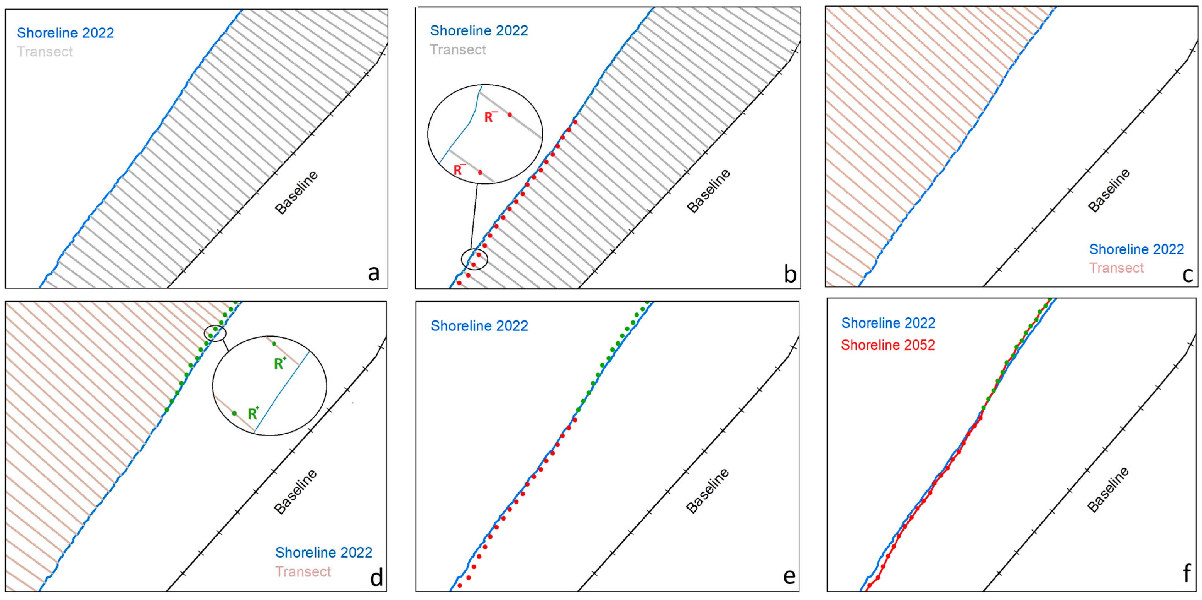
• Generation of transects: transects spaced 20 m apart were generated using DSAS, from the baseline to the 2022 reference shoreline.
• Projection of points on the land: after generating the transects, points were plotted along them towards land, spaced at a specific distance, using the ArcGIS ‘Create Point on Lines’ extension. The distance corresponded to the negative values of the projected retreat “R⁻” over a period of 30 years, as calculated by the Durand and Heurtefeux equation.
• Creation of transects oriented towards the sea: transects were also created for the reference 2022 shoreline, this time oriented towards the sea. These were spaced in the same way as the transects towards land.
• Projection of points towards the sea: the positive values of the projected retreat “R⁺” over 30 years were used to project points towards the sea along these transects.
• Overlay of points: Once all points are created, they are overlaid to obtain a complete visualisation of the projected shoreline at the 30-year horizon.
• Digitisation of the shoreline position in 2052: the shoreline position in 2052 was digitised by connecting the points created.

After plotting the shorelines for both time horizons based on the two IPCC projections, they then had to be compared to the situation on the ground. This step was carried out using the Lidar 2022 DTM provided by the Vendée department to identify low-lying areas and ensure that the projections were limited to the dune ridge, as for the study area, without going over the rocky platforms or other geomorphological or geological features. Following these steps, the 100-year projection shoreline was mapped using the 2052 reference shoreline in place of the 2022 reference shoreline, using the related predicted recession values.

The projected evolutionary shoreline trend was then divided into nine classes, represented by coloured boxes of 20 × 250 m along the coast. Shades of red were used for areas predicted to recede and shades of blue for areas predicted to advance. The white areas represent longitudinal protection structures. These were not considered for the projection since they were considered fixed in this projection test.

3.4.2. Estimation of Error

Projecting a shoreline to a given date consists of (i) extrapolating past evolutionary trends for the shoreline and (ii) estimating shoreline retreat due to sea level rise. Uncertainties related to both the choice of methodology and the choice of data are involved with each of these parameters [53,64]. An uncertainty analysis was therefore carried out based on these criteria:

• Data error for the four variables used in the Durand and Heurtefeux equation [59] (

  Table 5. Uncertainty relating to the data.

  Variables	Uncertainty of shoreline position (pixel error, orthorectification error, digitisation error)	This study	Uncertainty	1950–2022	1992–2022	Uncertainty by projection horizon	2052	2122
  				6 cm/an	15 cm/an		450 cm	600 cm
  	Uncertainty related to the average annual sea level rise since 1950 (E20)	Ferret (2016) [63]		1950–2014			2052	2122
  				0.022 cm/an			0.66 cm	2.2 cm
  	Uncertainty about slope (DTM error)	Lidar provided by the Vendée department (2022)		2022			2052	2122
  				15 cm	15 cm		15 cm	15 cm
  	Uncertainty related to the estimation of future sea level rise (E21)	IPPC (2022) SSP2-4.5 (median)	Projection	2052	2122		2052	2122
  				21 cm	23 cm		9 cm	33 cm
  		IPPC (2022) SSP5-8.5 (secure)		64 cm	90 cm		10 cm	30 cm

  ): the calculation of uncertainty associated with the position of the shoreline was based on the results of the error in the overall position of the shoreline, as shown previously in Table 3. In addition, uncertainty relating to variable E20 was derived from work carried out by Ferret [63]. With regard to uncertainty related to slope, this value was deduced from the error present in the Lidar 2022 DTM data provided by the Vendée department. Finally, to estimate the uncertainty of variable E21 relating to future sea level rise, the IPCC assessments were used as a reference.
• Error relating to the shoreline projection based on the results of the comparison between the digitised and projected shorelines for 2022 (

  Table 6. Uncertainty relating to the shoreline projection test: statistical differences between projected and digitised shorelines in 2022.

  Littoral Cells (LCs)	Mean Deviation (m)	Annualised Mean (m)	Max (m)	Min (m)	Standard Deviation (m)	Total (m)	Total Number of Transects
  LC1-A	15.29	0.59	39.49	1.06	11.34	886.65	58
  LC1-B	0.00	0.00	0.00	0.00	0.00	0.00	0
  LC1-C	3.31	0.13	10.06	0.40	2.65	109.32	33
  LC2-A	11.39	0.44	49.82	0.06	10.85	1685.64	148
  LC2-B	0.00	0.00	0.00	0.00	0.00	0.00	0
  LC2-C	6.13	0.24	24.76	0.03	5.60	337.12	55
  LC2-D	18.26	0.70	29.49	1.39	7.86	255.69	14
  LC2-E	22.48	0.86	54.64	0.07	12.10	8316.74	370
  LC2-F	110.09	4.23	270.23	0.05	85.44	15,082.25	137
  Overall coastline studied	32.73	1.26	270.23	0.03	50.71	26,673.41	815

  ): the aim of the methodology was to quantify the past evolution of the shoreline and project it to the 2022 horizon, a year for which the position of the shoreline is known. The method consisted of first calculating an average evolutionary trend over a period of 26 years (1974–2000). The parameters used in the Durand and Heurtefeux formula, comprising extrapolation, slope, and rise in sea level since 1950 and predicted for 2022, were used for a 22-year projection of the shoreline based on the position of the shoreline in 2000. The uncertainty was then evaluated according to the mean annual difference between the two shoreline positions (digitised and projected in 2022) and normalised by the number of years used in the projection.

Uncertainty relating to both the data and the projection testing (

Table 7. Overall uncertainty by projection horizon.

	2052	2122
Data error (m)	4.50	6.01
Projection test error (m)	37.76	125.88
Overall error (m)	38.03	126.02

) was considered when evaluating the overall uncertainty about the future position of the shoreline. The uncertainty was calculated as the square root of the sum of the squares of the two types of error.

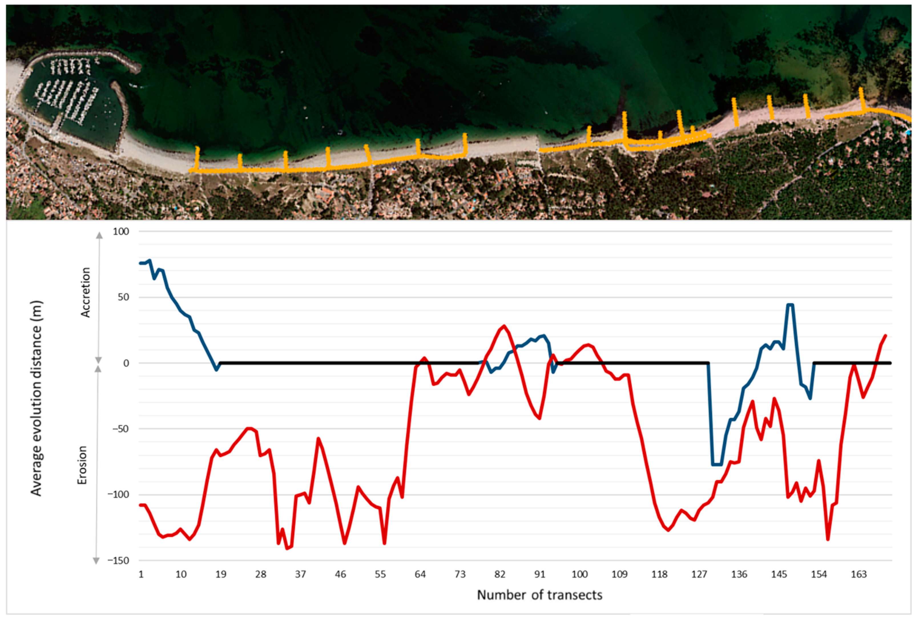
3.4.3. Proximity of Stakes to the Projected Shorelines

Only one type of stake was considered for this study—buildings. The data are from the IGN (French National Geographic Institute) BD-Parcellaire 2023. The analysis focuses on the surface area these buildings occupy entirely or partially within the uncertainty band. This band is defined as a buffer zone where future shoreline retreat is anticipated. It lies on both sides of the projected shorelines; the most pessimistic IPCC scenario (SSP5-8.5) was chosen in each case. The zone will extend over ±38 m by 2052 and rise to ±126 m by 2122. The intersection where the buffer zone comes into contact with a building indicates buildings that will potentially be affected by the retreating shoreline.

4. Results

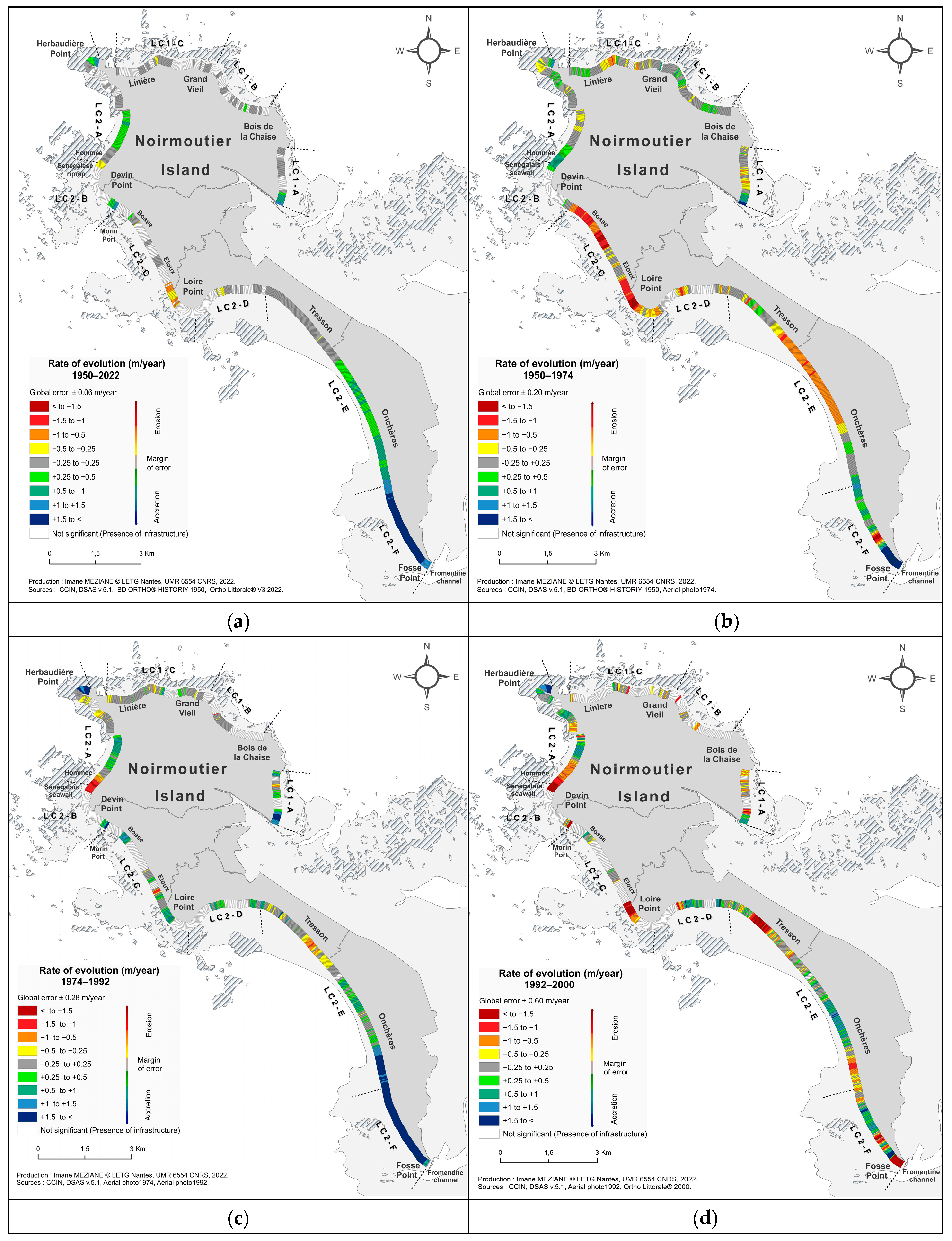
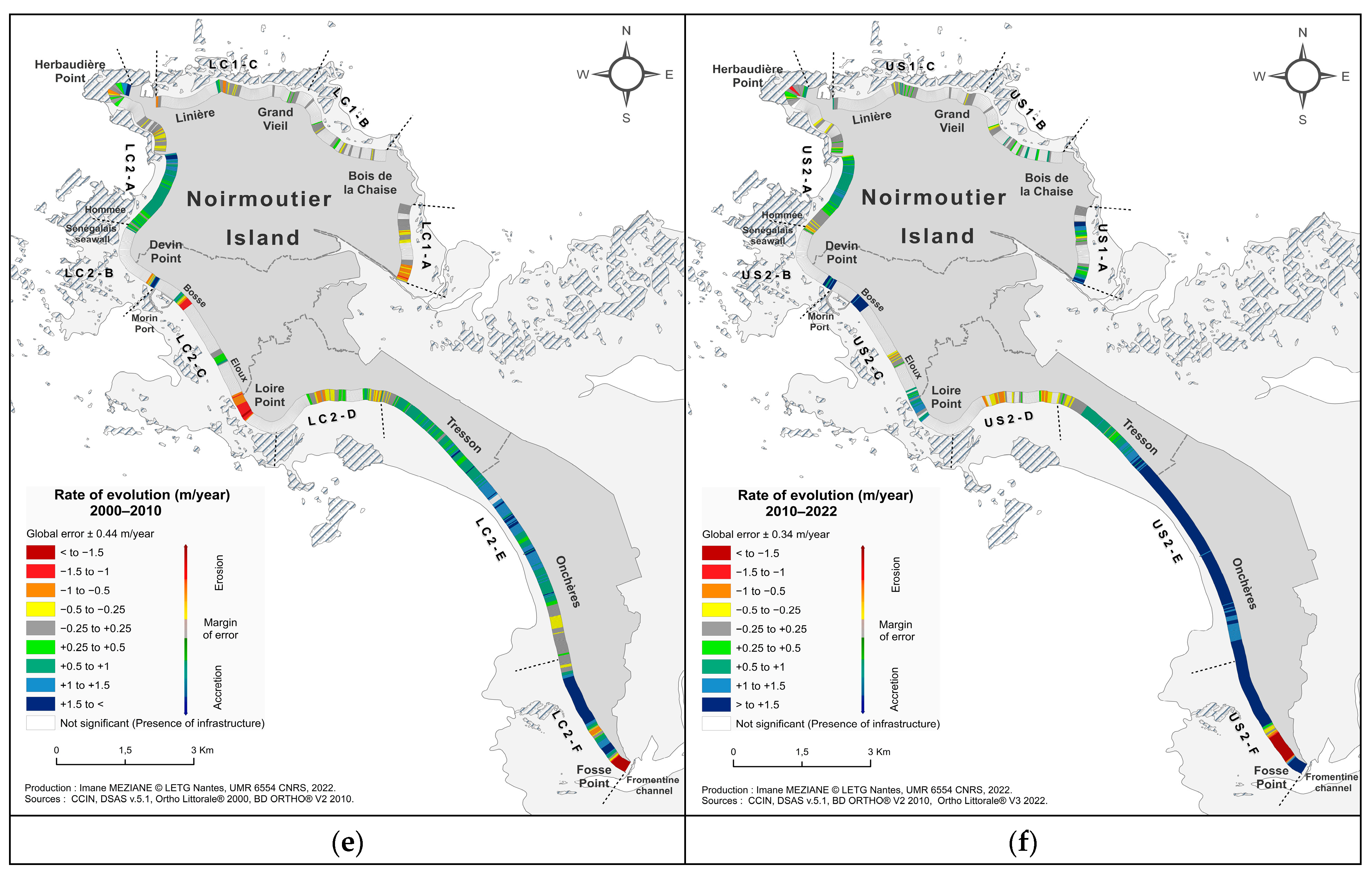
4.1. Analysis of the Shoreline Linear Evolution

An analysis of the linear evolution of the Noirmoutier shoreline in the period 1950–2022 revealed significant variation. A total of 47% of the Noirmoutier shore with no longitudinal structures was subject to accretion over 72 years. The overall average rate of accretion was approximately +0.57 ± 0.06 m/year (Figure 5a), corresponding to an average advance of +40.63 ± 4.32 m over the period. Between 1950 and 1974 (Figure 5b), 54% of the shoreline studied was subject to erosion, with an average retreat rate of −0.12 ± 0.20 m/year, i.e., −2.96 ± 4.8 m.

Between 1974 and 1992 (Figure 5c), an overall progression trend was observed, with 48% accretion and 23% retreat, while longitudinal structures were present along 29% of the shoreline. The average progradation rate was +1.10 ± 0.28 m/year, with LC2-F as high as +120 ± 5.04 m, and the maximum retreat was observed at the southern end of LC2-A at −1.59 ± 0.28 m/year, revealing the presence of disturbances linked to the state of disrepair of the Sénégalais seawall [65]. The construction of the port of Morin accelerated accretion in the areas to the south and immediate north of the port at a maximum rate of +2.63 ± 0.28 m/year, equivalent to +46.48 ± 5.04 m over the period in question.

In contrast to the above period, extensive erosion was observed between 1992 and 2000, with an overall average retreat rate of −0.2 ± 0.60 m/year, i.e., −1.65 ± 4.8 m (Figure 5d). The storms that occurred in October and December 1999 probably contributed to the trend. Across the whole length of shoreline studied, 33% was subject to erosion, while 30% experienced accretion. Longitudinal structures were observed along 37% of the shoreline.

Between 2000 and 2010, the sections of the coastline without longitudinal structures (38%) experienced progradation, i.e., 43% of the overall coast, with an average progradation of +5.58 ± 4.4 m, i.e., a rate of +0.54 ± 0.44 m/year (Figure 5e). The progradation may be explained by the introduction of soft defence measures, in particular a sand nourishment programme in cells 2-A, 2-B, and 2-E (+3000 m³ in Lutins, +43,700 m³ in Hommée, and +31,000 m³ in Tresson). LC2-F registered a maximum progradation of +16.02 ± 4.4 m, leading to the formation of a sandy spit. By contrast, LC2-C showed a recession of −4.79 ± 4.4 m despite successive replenishment operations to a total volume of more than 143,900 m³ for the period and despite a succession of protective installations such as stone revetments and groynes. These measures failed to prevent erosion [12]. The erosion trend could be linked to the negative effects of the coastal drift being interrupted by the construction of the port at Morin, which restricted the amount of sediment deposited in this area. Indeed, the port acts as a barrier that reduces sediment input down-drift and causes accumulation up-drift.

Between 2010 and 2022, extensive progradation was observed in 47% of the study area at an average rate of approximately +1.45 ± 0.34 m/year, or +16.26 ± 4.08 m (Figure 5f). However, 12% of the shoreline retreated, 41% of which was artificial. The maximum accretion rate was recorded in the north of LC2-F, with +13.36 ± 0.34 m/year (+150.13 ± 4.08 m). Despite negative fluctuations, this sector recorded an average advance of +44.06 ± 4.08 m. The variations can be explained by the random oscillations of the Fromentine channel [66], where there are no developments to disturb the coastal dynamics. In addition, a reversal of the trend towards accumulation was observed in LC2-C, with a progradation of +11.89 ± 4.08 m due to a sand nourishment programme (24,000 m³ at La Bosse in 2011/2012) and the construction of two stone revetments (at Éloux in 2010 and Loire Point in 2013).

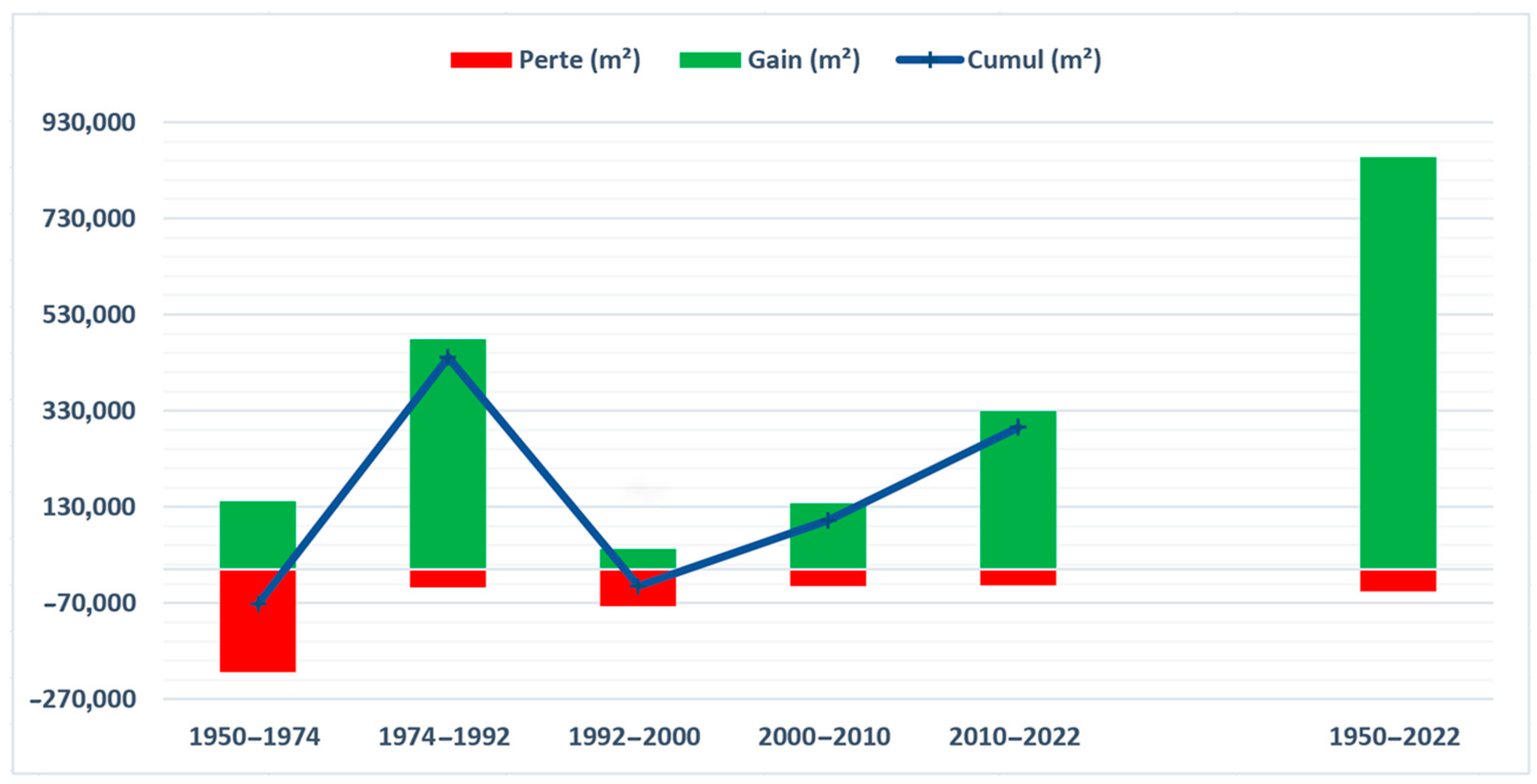
4.2. Analysis of the Shoreline Surface Evolution

The results reveal that the island of Noirmoutier experienced phases of both erosion and accretion, marked by significant changes over various periods (Figure 6). The overall surface balance for the 72-year period between 1950 and 2022 is +810,422 ± 49,936 m². Different phases were observed during this period. Between 1950 and 1974, the island experienced marked erosion with a negative balance of −71,770 ± 130,577 m². This erosion phase was followed by a period of recovery between 1974 and 1992, with a positive balance of +441,087 ± 111,095 m². The period between 1992 and 2000 is particularly interesting, as there was a shift towards another phase of erosion. The surface balance during this period recorded a loss of −34,805 ± 62,167 m². Since 2000, the island has shown steady surface growth, with a dominant sedimentation and expansion trend. Between 2000 and 2010, the surface balance was positive with +101,770 ± 40,290 m², and this trend increased between 2010 and 2022 with a balance of +295,588 ± 33,324 m².

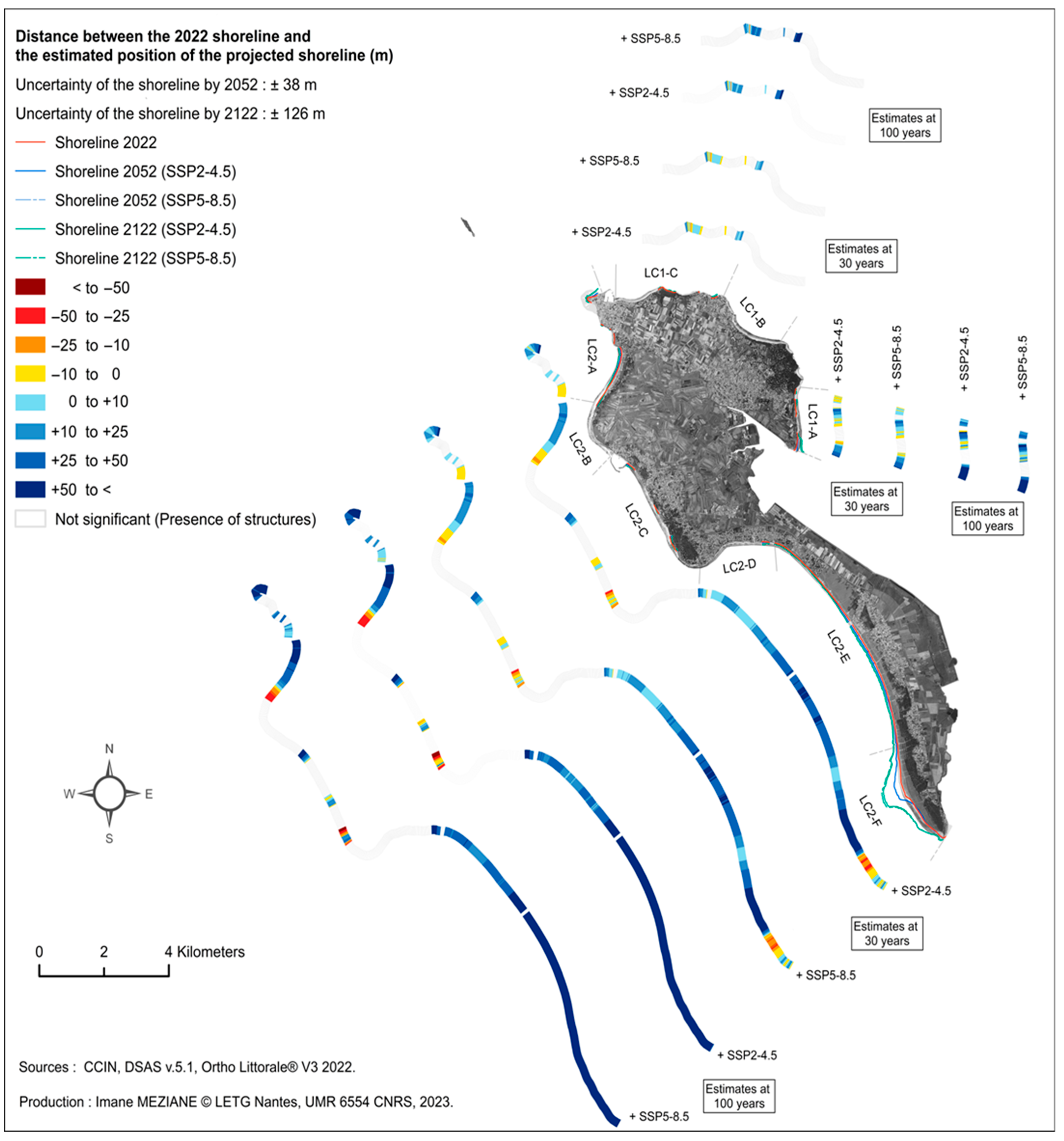
4.3. Prospective Analysis of the Shoreline over 30 Years and 100 Years

4.3.1. Comparison of the Two Projection Tests

A comparison of the shoreline evolution projections to 30-year and 100-year horizons, as shown in

Table 8. Projection of the shoreline evolution to the 30-year and 100-year horizons according to the secure scenario (SP5-8.5), as an illustration, considering the maintenance or absence of longitudinal coastal structures.

A. Distance between the 2022 and 2052 Shorelines According to the SP5-8.5 Scenario.
			The average distance of evolution (m) over 30 years (2022–2052)
Test	Observation period		LC1-A	LC1-B	LC1-C	LC2-A	LC2-B	LC2-C	LC2-D	LC2-E	LC2-F
1	1992–2022 (presence of longitudinal coastal structures)		+58	/	+33	+10.83	−7.71	+3.05	+12.04	+28.33	+76.46
2	1950–1974 (absence of longitudinal coastal structures)		+7.46	+10.49	+4.34	+7.7	+13.53	−20.4	+3.46	−4.82	+45.17
B. Distance between the 2022 and the 2122 shoreline according to the SP5-8.5 scenario.
			The average distance of evolution (m) over 100 years (2022–2122)
Test	Observation period		LC1-A	LC1-B	LC1-C	LC2-A	LC2-B	LC2-C	LC2-D	LC2-E	LC2-F
1	1950–2022 (presence of longitudinal coastal structures)		+62.52	/	+30.03	+36.55	−34.81	+10.18	+62.86	+70.07	+351
2	1950–1974 (absence of longitudinal coastal structures)		+36.61	+46.3	+26.43	+33.65	+53.91	−51.95	+37.07	−7.08	+181

as an illustration of the secure scenario (SP5-8.5), revealed significant differences between the two tests. The projections arising from the 1950–1974 observation period (test 2) produced evolution rates different from those resulting from the 1992–2022 period (test 1) for the 30-year horizon and from the 1950–2022 period (test 1) for the 100-year horizon. In addition, in the results of the second test, the projection for the 2022 shoreline based on the period between 1950 and 1974 showed significant deviations from what was actually observed. The average deviation was actually 49 m, with a maximum value of around 150 m recorded at Fosse Point, where there was an active sediment dynamic caused by the Fromentine channel and where a sandy spit is present.

To highlight the differences observed between the two tests, a zoom on a specific sector has been selected as an example. Figure 7 shows that the distance projected on the basis of historic changes between 1950 and 2022 and based on the digitised 2022 shoreline in test 1 is characterised by a progradation of the shoreline by about +10 m, where there are no longitudinal protection structures. The distance projected on the basis of the historic changes between 1950 and 1974 and from the theoretical 2022 shoreline for test 2, on the other hand, is marked by a retreat of approximately −62 m over the entire sector studied.

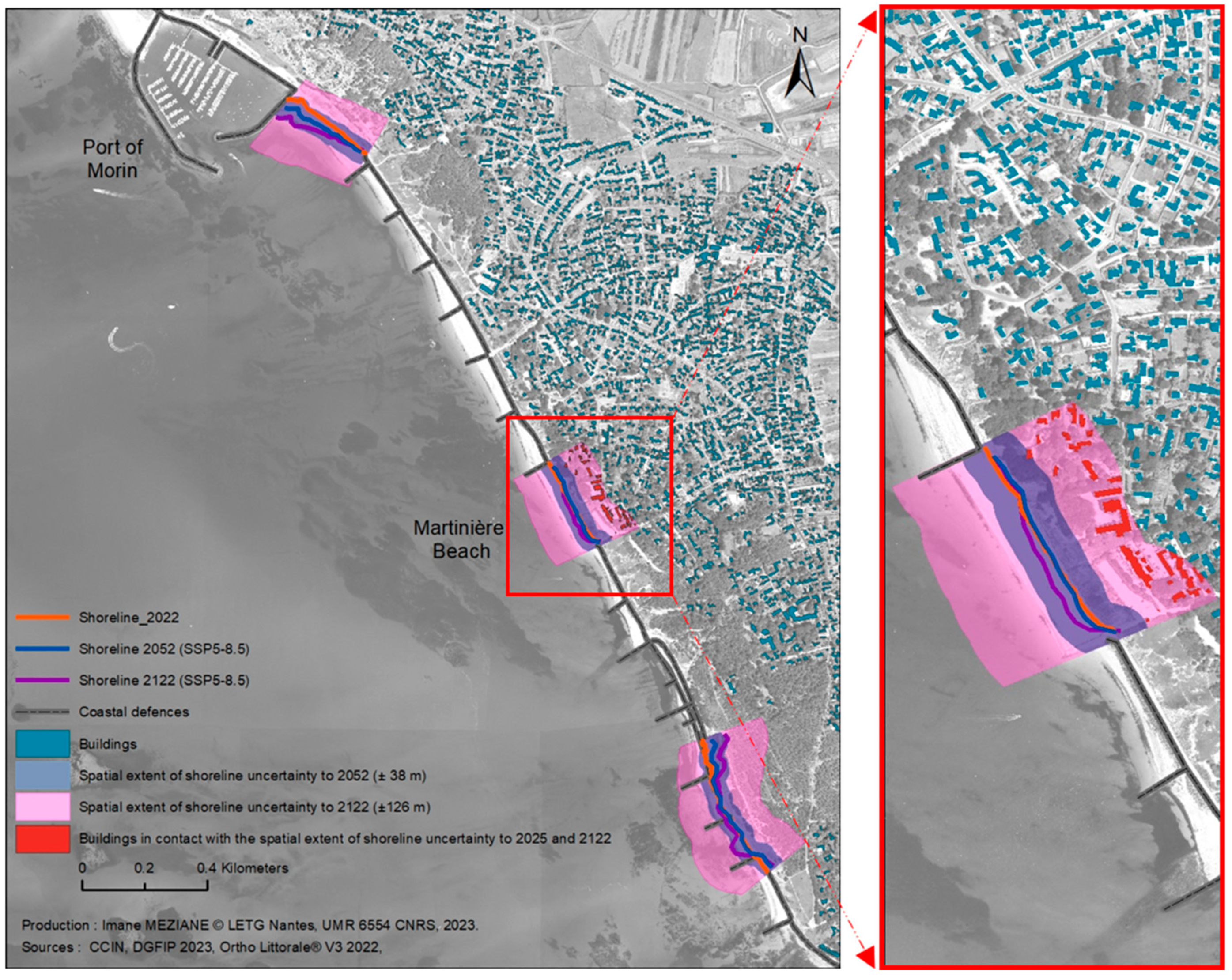
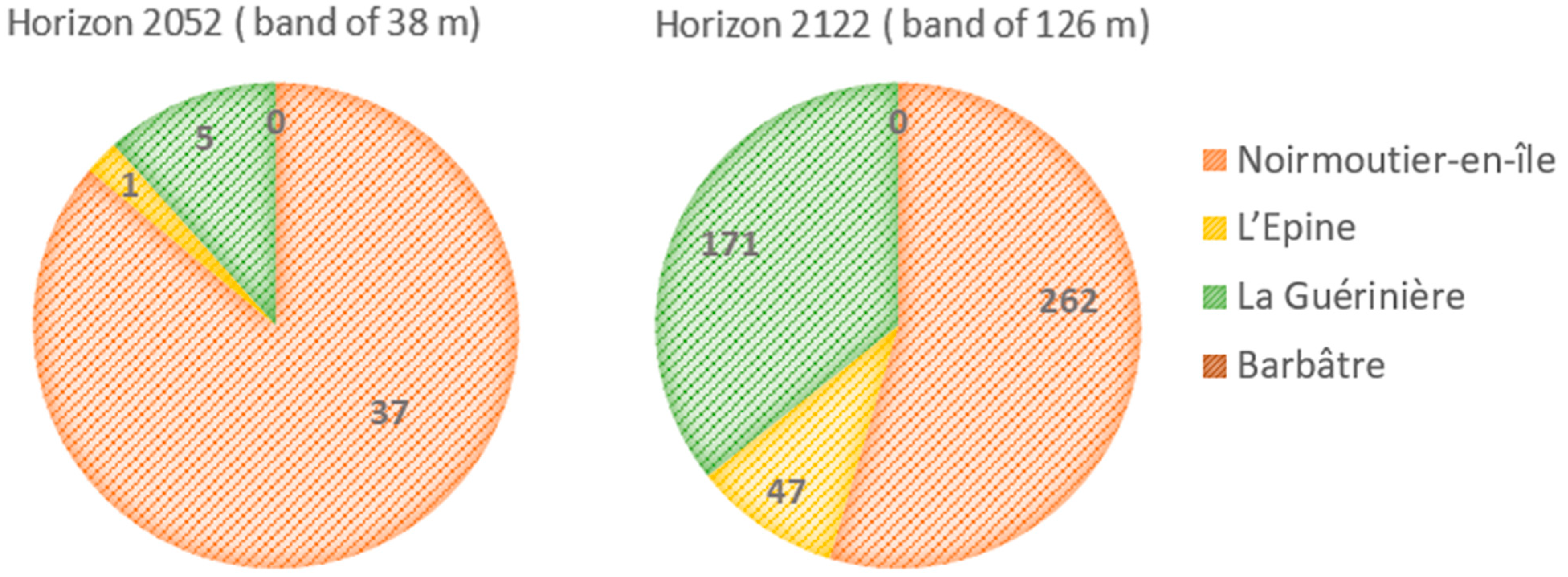
4.3.2. Prospective Mapping of the Noirmoutier Island Shoreline in 2052 and 2122

This section shows a map of local exposure to shoreline retreat over 30 years and 100 years, focusing on the scenario where the coastal structures are retained; this could be the result of a political decision to preserve the existing infrastructure.

Figure 8 shows the distance, calculated at 20-metre intervals, between the shoreline in 2022 and the projected shorelines for 2052 and 2122 for coastal stretches where there are no longitudinal protection structures and in line with IPCC scenarios SSP2-4.5 and SSP5-8.5. The most important observations to be drawn from the map are that accretion could be predominant in 2052, with a maximum estimated accretion of +242 m and a maximum estimated erosion of −32 m. The average erosion could be established at −8.5 m and the average accretion at +36 m. Projecting towards the horizon of 2122, the results indicate a significant increase in accretion to an estimated maximum of +706 m, while a maximum erosion could be estimated at −77 m. The mean erosion for this period could be −24.1 m, with a mean accretion of +112.3 m. It is important to note that these results are subject to differing levels of uncertainty. In comparison, the projected shoreline for the year 2122 exhibits a greater degree of uncertainty than that projected for the year 2052. Specifically, the uncertainty associated with the 30-year horizon is ±38 m, whereas the uncertainty for the 100-year horizon is ±126 m.

5. Discussion

5.1. Methodological Choices

The accuracy of shoreline evolution projections heavily depends on the methods and data utilized. Each methodological choice influences the results and reliability of predictions. This exploration of methodology is essential for understanding the analytical foundations of our findings and for correctly interpreting the implications of our forecasts for future coastal zone management in the face of environmental and climate change. It underscores the critical importance of every decision in constructing a robust and valid analysis of shoreline retreat.

5.1.1. Choice of Method for Estimating Surface Uncertainty in the Shoreline Evolution

The choice of method for estimating surface uncertainty in shoreline evolution was based on the use of the length of the coastline, which enabled direct, accurate measurement of the uncertainty. Considering the actual geometry of the coastline, this method provided a more accurate and representative estimation of how the coastline has evolved. It also enabled a holistic approach to be adopted by identifying local variations and peculiarities of the study zone, thereby ensuring the reliability of the results. By combining these elements, the method provided a more complete evaluation of the uncertainty associated with coastal dynamics.

5.1.2. Choice of Shoreline Projection Method

The most commonly used method of estimating shoreline retreat due to sea level rise is the Bruun rule [9], based on the hypothesis that beaches have a sediment equilibrium profile that translates variations in the sea level without changing shape. Because of this, it can only be used for sandy areas and fails to consider the effects of longshore drift [67]. It has actually been subject to strong criticism [68,69]. Various studies have concluded that although Bruun’s rule may be suitable for qualitative evaluations on a regional level, its relatively weak quantitative precision and unreliability mean it is inappropriate for evaluations at the local level, where more reliable estimations are required [70,71]. Another method by Ranasinghe et al. [60] was proposed as an alternative to Bruun’s rule; known as the Probabilistic Coastline Recession Model (PCR), it uses an impact model based on physical processes. It enables probabilistic extrapolation of the future position of a coastal stretch, considering both extreme events and periods of dune rehabilitation. It is more complicated to implement and not fully tested, providing margins of uncertainty based on the identification of morphogenic events, their impact on the coastline, and the non-consideration of a succession of less morphogenic events that could cumulatively result in severe erosion [64]. Our decision was motivated by practical considerations and data availability, and we finally settled on the Durand and Heurtefeux method [59], inspired by Bruun’s rule. This approach is based on measuring historic trends to evaluate future shoreline evolution at the local level. It considers past processes that have contributed to the localisation of the shoreline and also incorporates sea level rise in its projections. Although it is an unequivocally hypothetical method since it fails altogether to consider the dynamic effects of an acceleration in sea level rise (increase in frequency and intensity of storms, potential changes in sediment flow, beach profile) [59], it can provide estimates of shoreline retreat due to sea level rise without the complexities associated with the Ranasinghe et al. [60] method.

5.1.3. Choice of Historic Period

The discrepancies noted between the projected 2022 shoreline based on the period 1950–1974 and the digitised 2022 shoreline call into question both the reliability of the projection method used and the ability of the observation period to capture all the factors that could have affected shoreline evolution up to 2022. In addition, the differences observed between the results of the two tests highlight the importance of choosing the right historic period on which to base the estimation of future shoreline evolution, suggesting that historic conditions such as environmental change, climate change, and human intervention during this period may have considerably influenced the accuracy of the projections. Extrapolating historical trends, in fact, assumes that the evolution of a shoreline in the future will be subject to the same processes the shoreline is currently experiencing (i.e., the influence of local geology, waves, sea level rise, and sedimentary budgets) [72].

It is also pertinent to note that the projections in test 2 were carried out on a 2022 shoreline, which was itself produced as a projection. This too could help explain the discrepancies observed between the two tests and underline the complexity of predicting shoreline evolution, since it depends not only on the selected observation period but also on the data used as the basis for prediction.

5.1.4. Uncertainty Relating to the Estimation of Future Sea Level Rise (E21)

As mentioned previously, the recommended sea level rise projections for mapping local exposure to shoreline retreat over 30 and 100 years are the middle-of-the-road SSP2-4.5 and the secure SSP5-8.5.

In the short term, the retreat scenarios are relatively low. This is because the predictions for sea level rise are constant, with SSP2-4.5 indicating an increase of only 20 cm and SSP5-8.5 only 23 cm. The differences are more marked over the longer term, with SSP2-4.5 predicting 64 cm and SSP5-8.5 predicting 89 cm in 100 years’ time. These discrepancies suggest more contrasting scenarios when it comes to the long-term evolution of the shoreline. They also give rise to a considerable increase in uncertainty depending on the time horizon; this stems from the fact that the longer the period considered, the more extensive the uncertainties. In addition, estimates of future sea level rise are based on records of observations from between 1995 and 2014, which adds to the uncertainty. This is a relatively short period, so it cannot fully consider the natural variability of the sea level over longer periods, introducing the uncertainty that this period is insufficiently representative for making future projections.

5.1.5. Uncertainty Relating to Slope Estimation

In terms of using the Durand and Heurtefeux method [59] to evaluate shoreline retreat, one key variable requires determination of the slope of the beach, which is defined as the slope of the lower beach and the higher part of the upper beach expressed as a percentage, from the crest of the berm to the first pre-littoral sand bar, approximately 1 m away in a microtidal environment. However, the exact meaning of the term ‘beach slope’ leads to a fundamental problem [73,74,75,76].

For the present study, it was essential to adapt the definition of slope to the specific characteristics of the macrotidal Noirmoutier coast. This could potentially have affected the positioning of reference points to identify the slope, and consequently, the slope was delimited by the high astronomical tide level (HAT) and the low astronomical tide level (LAT). The Lidar 2022 DTM supplied by the Vendée department, however, was unable to ascertain the LAT because it does not cover this limit. Consequently, the beach limit was based on the lowest line that could be extracted from the model.

This was the best possible approach given the data available, but it is important to note that the beach slope can considerably alter the final evaluation of the recession [70]. This circumstance illustrates how critical it is to achieve the most accurate definition of the slope in a way that is appropriate for the purpose of the study in order to reduce uncertainty about shoreline retreat within a given period to a minimum.

5.1.6. Choice of Using L_max in the Durand and Heurtefeux Method

A number of recent works, including the methodological guide for Coastal Risk Prevention Plans (PPRL) [77], recommend adding a maximum retreat (L_max), corresponding to the retreat observed following an extreme event, to the long-term trend in order to estimate the future position of the shoreline [78]. Likewise, Audère and Robin [40] suggest estimating the value of L_max to consider the impact of certain morphogenic events, the estimate being based on an observation of only two storms, i.e., Lothar and Martin (1999) and Xynthia (2010), due to the lack of available data. The value thus obtained for L_max can then be added to the historic trend together with the future sea level rise.

In spite of the recommendation, however, it is prudent to consider the limits and uncertainties associated with these methods. The value of L_max can vary considerably from one coastal area to another depending on the local geography, and the specific characteristics of the two selected storms cannot fully represent the overall range of potential scenarios; this means that the real impact of future events could be either overestimated or underestimated.

In this particular study, adding L_max to the Durand and Heurtefeux formula for predicting the shoreline could mean doubling the effects of past storms when evaluating the future evolution of a shoreline, since the maximum shoreline retreat associated with these extreme events has already been considered in the historical evolution of the shoreline. The limited availability of data from past events, as noted in this study, may also introduce significant uncertainty in estimating L_max, negatively affecting the reliability of the value.

Taking all these considerations into account, the decision was made not to add L_max to the shoreline projection method based on the Durand and Heurtefeux approach. It is important to note that every approach has its advantages and its limitations; the final choice depends on the study specifications and the data available.

5.1.7. Inclusion or Exclusion of Coastal Protection Structures for Mapping

This issue of whether to include coastal protection structures was an important part of the discussion concerning shoreline retreat projections over 30 and 100 years. Initial observations suggested that in scenarios where protection structures were maintained, the impacted areas may appear relatively limited, at least in the short term. Note, however, that the impact they have could be significantly higher in the longer term, highlighting their increasing relevance over time.

With this in mind, the issue of the sustainability of protection structures becomes more pressing and requires careful consideration since various factors come into play, such as climate change, extreme events, and even the simple fact that installations wear out over time. The cost of maintaining and reinforcing them may also be prohibitive for local authorities.

On the other hand, if coastal protection structures are not taken into consideration, the coastal areas would be exposed to increased risks of shoreline retreat. Without these structures, areas that were previously considered low-risk could face major challenges. This observation highlights the crucial importance of the existing protective structures in preserving coastal areas and reducing potential impacts. It does lead to the question, however, of whether these structures are able to cope with extreme events and the long-term effects of climate change, highlighting the need for continuous re-evaluation of their effectiveness and adaptability to ever-changing conditions. It also constitutes an incentive to explore sustainable alternatives, such as nature-based approaches and planned relocation strategies.

5.2. Most Impacted Sectors

The most impacted sectors, irrespective of the issues involved, can be synthesised in the following graph (Figure 9). Relative to the overall balance (erosion or accretion) evaluated in terms of surface area, the percentage representation of each coastal cell’s contribution to this total illustrates several key points:

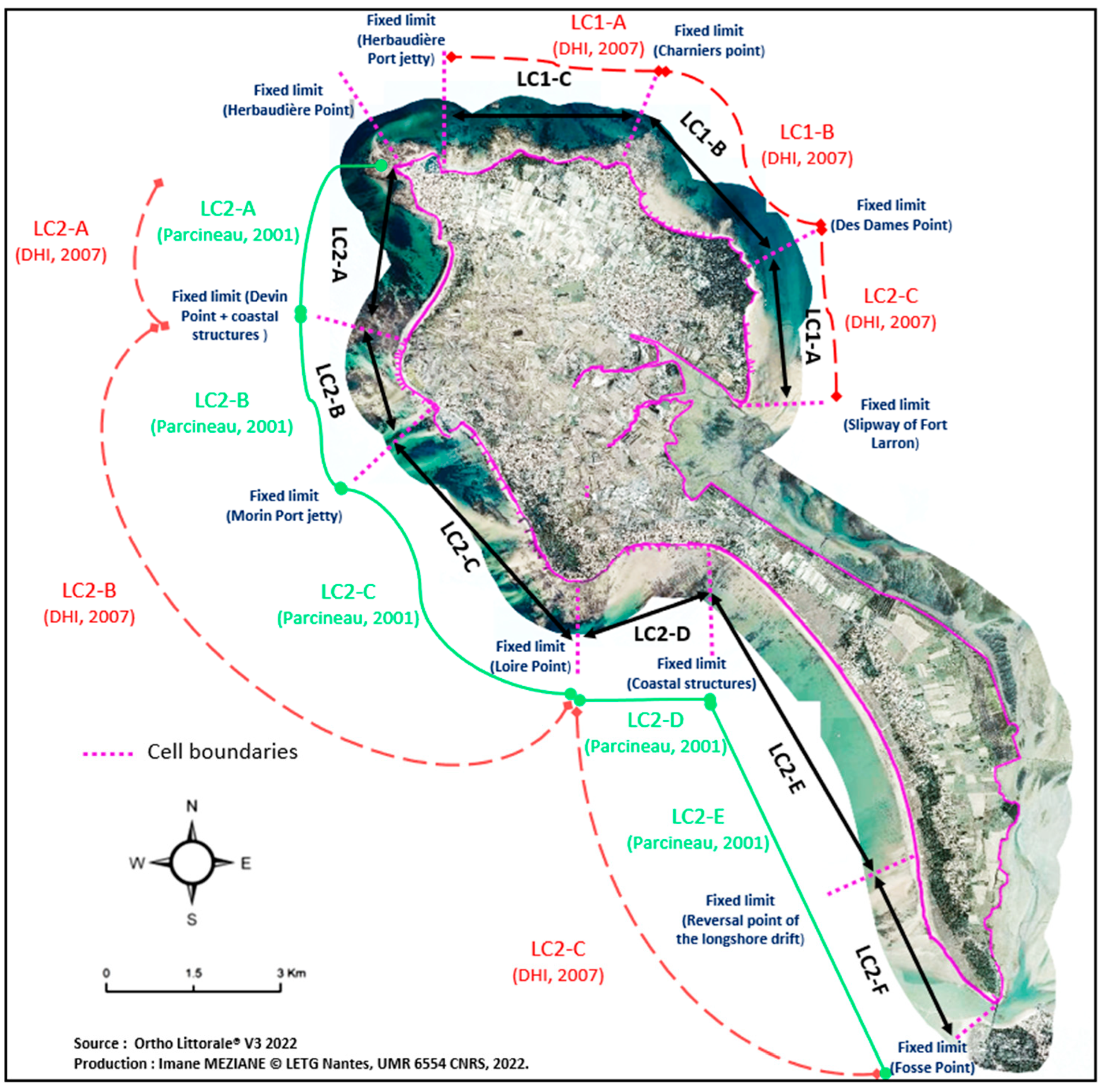
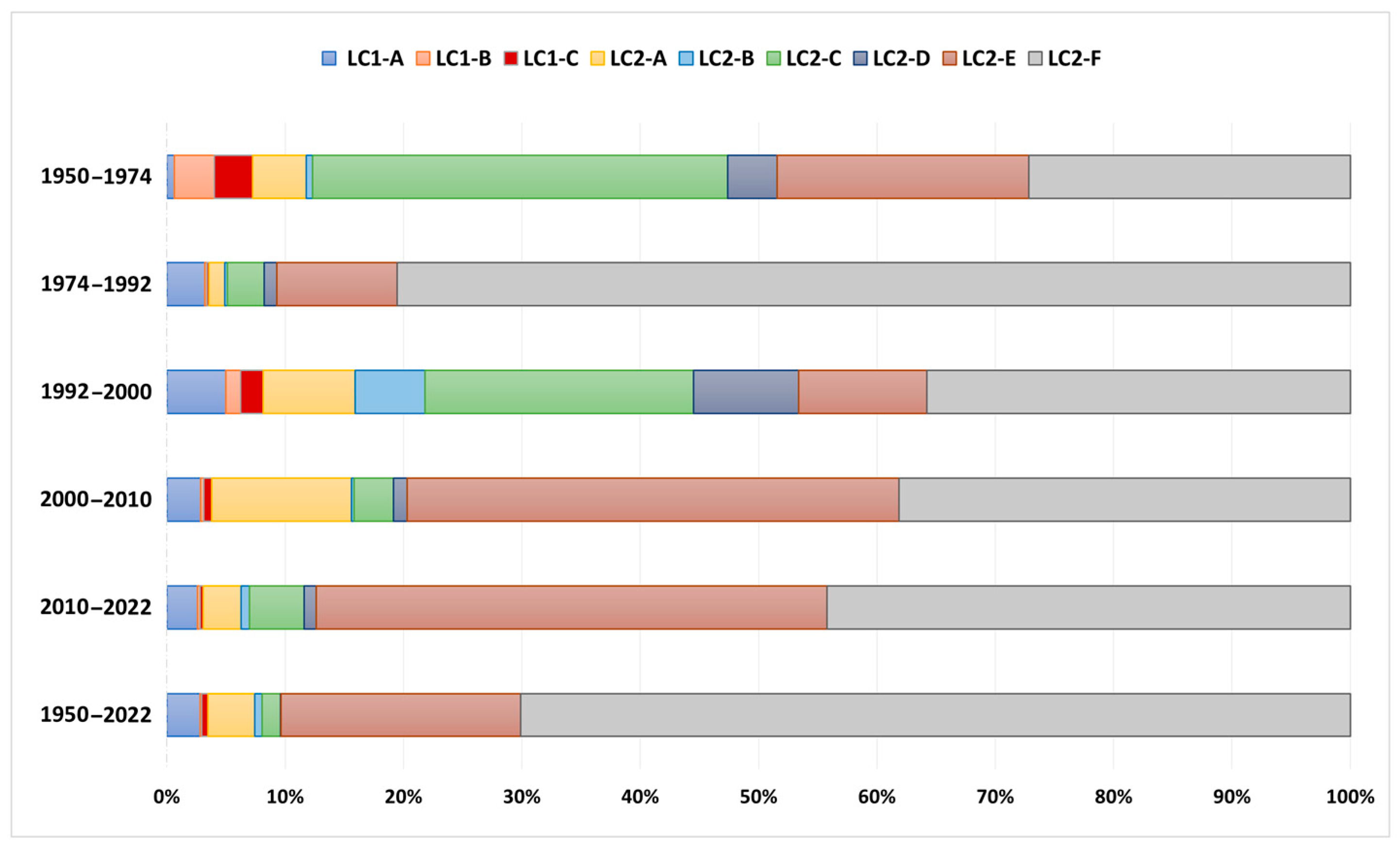
• The significant contribution of certain cells to the total balance. For instance, LC2-E showed a remarkable contribution to the overall balance, especially during the periods from 2000 to 2010 and 2010 to 2022. Indeed, each coastal cell exhibits a distinct behaviour that evolves at its own pace.
• Variations in contributions among different coastal cells over time. For example, LC2-F made a major contribution during the period 1974–1992, and its smallest contribution remains significant during the earlier period from 1950 to 1974. Other cells have minor contributions.
• These variations stem from both storm cycle variations and sand replenishment, as well as coastal defense development. For instance, LC1-B has seen a diminishing contribution over time, attributed in this case to an increase in protected coastline length. Thus, each case requires a thorough analysis of natural forces and human interventions.

However, the minor contribution of a particular coastal cell does not imply an absence of issues related to the location of stakes. This underscores the importance of considering retro-littoral issues within these cells.

5.3. Operational Use of Results

The main results consist of creating erosion bands that can be used within the framework of climate resilience laws. For example, Figure 10 presents, in a specific sector, the principle of the intersection of future erosion bands with urbanisation stakes. The mapping shows areas that are particularly susceptible to shoreline retreat within 30 and 100 years, including a 38 m uncertainty band for the 30-year horizon and a 126 m band for the 100-year horizon. This visual representation enables spatial identification and projection of the areas and buildings that could be affected over time. For the four municipalities concerned in this article, the totality of the impacted urbanisation stakes is presented in Figure 11. In view of the secure scenario projection where coastal structures remain, 523 buildings could be affected by shoreline retreat between 2052 and 2122. During this period, the number of buildings across the whole study area will increase significantly, from 43 in 2052 to 480 in 2122. Indeed, the comparison between the 30-year and 100-year horizons shows a significant increase in the number of buildings affected as the shoreline retreats over time. Buildings that are less affected in the short term, most of them located in the municipalities of L’Epine and La Guérinière, will be increasingly affected moving towards the 100-year horizon.

State services in France are expecting this type of production to update the Local Urban Plans (PLU) in accordance with Article L121-22-2 of the Urban Planning Code, modified by Law No. 2021-1104 of 22 August 2021. This example illustrates that buildings will be impacted by shoreline retreat on both time horizons. Therefore, this work has a real operational purpose that can be replicated elsewhere in coastal municipalities in metropolitan France and overseas, where the Climate Resilience Law applies.

6. Conclusions

In conclusion, this study has been an opportunity to analyse the spatio-temporal evolution of the coastline of the island of Noirmoutier in its natural configuration and monitor changes brought in by successive coastal developments. The most significant erosion appears to have occurred during the period 1992–2000 in the far north of LC2-B, with an average retreat rate of −1.57 ± 0.60 m/year. Although the island has undergone phases of both erosion and accretion over the decades, the results for the entire period between 1950 and 2022 show a positive balance, with a net increase in overall surface area estimated at +81 ha. These observations suggest that natural processes and appropriate management strategies have helped stabilise and reinforce the island’s coastline.

The study has also highlighted the complexity of predicting the future evolution of the shoreline with accuracy and the importance of taking the uncertainties associated with this into account. Many factors have a considerable effect on the results of these predictions, including the projection method used, the historical period on which the analysis is based, the uncertainties associated with estimating the slope and future rise in sea level, and the decision whether or not to take coastal protection structures into account. Decision-makers and managers must take uncertainty into account when planning their adaptation strategies and managing coastal areas. To ensure a resilient response to future changes, it is important to consider a buffer zone around each projected shoreline as an area of uncertainty where future retreat can be anticipated.

In addition, in connection with current legislation, it is necessary to highlight the importance of the bands advocated in the Climate and Resilience Law, defining horizons at 30 years and 100 years. Compared to the Coastal Law of 1986, which prohibits construction within the 100-metre band, this study raises questions about the need for adaptation to address the evolving realities of the coastline. It suggests that some communities might adjust their regulations in response to this new law. The maps drawn up in the course of this study are indispensable tools for informing future regulatory documents and guiding public policy on dealing with foreseeable challenges within the next 30 and 100 years. This proactive approach will ensure that coastal communities endure in the face of climate change.

Finally, note that further studies will be required to refine these projections, considering additional data and improving the projection models used. Ongoing research in this field is essential to better understand the processes involved and provide more accurate predictions, which is critical for sustainable coastal management in the future.

References

1. Paskoff, R. Côte en Danger, Collection Pratiques de la Géographie; Masson: Paris, France, 1993; Volume 250. [Google Scholar]
2. Onerc. Le Littoral Dans le Contexte du Changement Climatique, la Documentation Française. 2015; Volume 180. Available online: https://www.ecologie.gouv.fr/sites/default/files/documents/ONERC_Rapport_2015_Littoral_WEB.pdf (accessed on 13 April 2024).
3. Meur-ferec, C.; Morel, V. L’érosion sur la frange côtière: Un exemple de gestion des risques. Nat. Sci. Soc. 2004, 12, 263–273. [Google Scholar] [CrossRef]
4. Callaghan, D.P.; Roshanka, R.; Andrew, S. Quantifying the storm erosion hazard for coastal planning. Coast. Eng. 2009, 56, 90–93. [Google Scholar] [CrossRef]
5. Oppenheimer, M.; Glavovic, B.C.; Hinkel, J.; van de Wal, R.; Magnan, A.K.; Abd-Elgawad, A.; Cai, R.; Cifuentes-Jara, M.; Deconto, R.M.; Ghosh, T.; et al. Sea level rise and implications for low-lying islands, coasts and communities. In IPCC Special Report on the Ocean and Cryosphere in a Changing Climate; Pörtner, H.-O., Roberts, D.C., Masson-Delmotte, V., Zhai, P., Tignor, M., Poloczanska, E., Mintenbeck, K., Alegría, A., Nicolai, M., Okem, A., et al., Eds.; Intergovernmental Panel on Climate Change: Geneva, Switzerland, 2019. [Google Scholar]
6. Rahman, M.K.; Crawford, T.W.; Islam, S. Shoreline Change Analysis along Rivers and Deltas: A Systematic Review and Bibliometric Analysis of the Shoreline Study Literature from 2000 to 2021. Geosciences 2022, 12, 410. [Google Scholar] [CrossRef]
7. Buchou, S. Quel Littoral Pour Demain? Vers un Nouvel Aménagement des Territoires Côtiers Adapté Au changement Climatique. Rapport Remis à Monsieur le Premier Ministre. 2019, Volume 108. Available online: https://www.lereportersablais.com/wp-content/uploads/2019/11/Rapport_Buchou_Extrait.pdf (accessed on 2 May 2023).
8. Apostolopoulos, D.; Nikolakopoulos, K. A review and meta-analysis of remote sensing data, GIS methods, materials and indices used for monitoring the coastline evolution over the last twenty years. Eur. J. Remote Sens. 2021, 54, 240–265. [Google Scholar] [CrossRef]
9. Bruun, P. Sea level rise as a cause of shore erosion. J. Waterw. Harb. Div. 1962, 88, 117–130. [Google Scholar] [CrossRef]
10. Luijendijk, A.; Hagenaars, G.; Ranasinghe, R.; Baart, F.; Donchyts, G.; Aarninkhof, S. The State of the World’s Beaches. Sci. Rep. 2018, 8, 6641. [Google Scholar] [CrossRef] [PubMed]
11. Cooper, A.; Masselink, G.; Coco, G.; Short, A. Sandy beaches can survive sea-level rise. Nat. Clim. Chang. 2020, 10, 993–995. [Google Scholar] [CrossRef]
12. Fattal, P.; Robin, M.; Paillart, M.; Maanan, M.; Mercier, D.; Lamberts, C.; Costa, S. Effets des tempêtes sur une plage aménagée et à forte protection côtière: La plage des Éloux (côte de Noirmoutier, Vendée, France). Norois 2010, 215, 101–114. [Google Scholar] [CrossRef]
13. Debaine, F.; Robin, M. A new GIS modelling of coastal dune protection services against physical coastal hazards. Ocean Coast. Manag. 2012, 63, 43–54. [Google Scholar] [CrossRef]
14. DHI. Analyses Météocéaniques au Large de Noirmoutier; DHI: Trentino, Italy, 2023; pp. 29–50. [Google Scholar]
15. CEREMA. Dynamique et Évolution du littoral, Fascicule 6 de la pointe de Chémoulin à la pointe de Suzac, Collection: Connaissances. 2019. Available online: https://doc.cerema.fr/Default/digital-viewer/c-16157 (accessed on 8 May 2023).
16. DHI; GEOS. Etude de Connaissance des Phénomènes D’érosion sur le LITTORAL vendéen. Rapport Final de la Tranche Ferme 2007. Volume 356. Available online: https://www.pays-de-la-loire.developpement-durable.gouv.fr/IMG/pdf/_50198_Erosion_du_littoral_vendeen_TF_FINAL.pdf (accessed on 22 April 2023).
17. Parcineau, L. Noirmoutier, Une île à Fleur D’eau: Évolution et Défense du Littoral de la Côte Ouest de l’île de Noirmoutier du 18e Siècle à Nos Jours 1. Master’s Thesis, Nantes University, Nantes, France, 1991. [Google Scholar]
18. Carter, R.W.G. Coastal Environments; Academic Press: Cambridge, MA, USA, 1988; p. 617. [Google Scholar]
19. Bray, M.; Carter, D.; Hooke, J. Littoral cell definition and budgets for central southern England. J. Coast. Res. 1995, 11, 381–400. [Google Scholar]
20. Frihy, O.E.; Shereet, S.M.; El Banna, M.M. Pattern of beach erosion and scour depth along the rosetta promontory and their effect on the existing protection works, Nile Delta, Egypt. J. Coast. Res. 2008, 244, 857–866. [Google Scholar] [CrossRef]
21. Anfuso, G.; Pranzini, E.; Vitale, G. An integrated approach to coastal erosion problems in northern Tuscany (Italy): Littoral morphological evolution and cell distribution. Geomorphology 2011, 129, 204–214. [Google Scholar] [CrossRef]
22. Boak, E.H.; Turner, I.L. Shoreline definition and detection: A review. J. Coast. Res. 2005, 214, 688–703. [Google Scholar] [CrossRef]
23. Moore, L.J. Shoreline mapping techniques. J. Coast. Res. 2000, 16, 111–124. [Google Scholar]
24. UNESCO-CSI. Environment and Development in Coastal Regions and in Small Islands. Available online: http://www.unesco.org/csi/pub/info/info410.htm (accessed on 15 May 2023).
25. Zemmour, A. Étude de l’évolution des Littoraux Dunaires de la Côte d’Opale à Différentes Échelles de temps: Analyse de leur Capacité de Régénération Post-Tempête. Thèse de Doctorat, Université du Littoral Côte d’Opale, Wimereux, France, 2019. Available online: https://theses.hal.science/tel-02270709 (accessed on 23 March 2022).
26. Dolan, R.; Fenster, M.S.; Holme, S.J. Temporal Analysis of Shoreline Recession and Accretion. J. Coast. Res. 1991, 7, 723–744. [Google Scholar]
27. Crowell, M.; Leatherman, S.P.; Buckley, M.K. Historical shoreline change: Error analysis and mapping accuracy. J. Coast. Res. 1991, 7, 839–852. [Google Scholar]
28. Durand, P. Approche Méthodologique Pour L’analyse de L’évolution des Littoraux Sableux par Photo-Interprétation. Exemple des Plages Situées Entre les Embouchures de l’Aude et de l’Hérault (Languedoc, France). Photo-Interprétation, 2000/1-2, 3-18. Available online: http://geoprodig.cnrs.fr/items/show/190158 (accessed on 2 July 2023).
29. Morton, R.A.; Miller, T.L. National Assessment of Shoreline Change—Part 2: Historical Shoreline Changes and Associated Coastal Land Loss along the US Southeast Atlantic Coast; U.S. Geological Survey Open-File Report; U.S. Geological Survey: Reston, VA, USA, 2005; p. 1401. Available online: http://pubs.usgs.gov/ (accessed on 30 September 2023).
30. Hapke, C.J.; Reid, D.; Richmond, B.M.; Ruggiero, P.; List, J. National Assessment of Shoreline Change: Part 3: Historical Shoreline Changes and Associated Coastal Land Loss Along the Sandy Shorelines of the California Coast; U.S. Geological Survey Open-File Report; U.S. Geological Survey: Reston, VA, USA, 2006; Volume 79, p. 1219.
31. Genz, A.S.; Fletcher, C.H.; Dunn, R.A.; Frazer, L.N.; Rooney, J.J. The Predictive Accuracy of Shoreline Change Rate Methods and Alongshore Beach Variation on Maui, Hawaii. J. Coast. Res. 2007, 231, 87–105. [Google Scholar] [CrossRef]
32. Del Río, L.; Gracia, F.J.; Benavente, J. Shoreline change patterns in sandy coasts. A case study in SW Spain. Geomorphology 2012, 196, 252–266. [Google Scholar] [CrossRef]
33. Juigner, M.; Robin, M.; Paul, F.; Maanan, M.; Debaine, F.; Le Guern, C.; Gouguet, L.; Baudouin, V. Cinématique d’un trait de côte sableux en Vendée entre 1920 et 2010. Méthode et analyse. Dyn. Environnementales Méthode Anal. 2012, 30, 29–39. [Google Scholar]
34. Grenier, A.; Dubois, J.M.M. Evolution littorale récente par télédétection: Synthèse méthodologique. Pho-Interprétation 1990, 6, 3–16. [Google Scholar]
35. Anfuso, G.; Bowman, D.; Danese, C.; Pranzini, E. Transect based analysis versus area based analysis to quantify shoreline displacement: Spatial resolution issues. Environ. Monit. Assess. 2016, 188, 568. [Google Scholar] [CrossRef] [PubMed]
36. Himmelstoss, E.A.; Henderson, R.E.; Kratzmann, M.G.; Farris, A.S. Digital Shoreline Analysis System (DSAS) Version 5.1 User Guide; U.S. Geological Survey Open-File Report; U.S. Geological Survey: Reston, VA, USA, 2021; Volume 104, p. 1091. [CrossRef]
37. Houser, C.; Hapke, C.; Hamilton, S. Controls on coastal dune morphology, shoreline erosion and barrier island response to extreme storms. Geomorphology 2008, 100, 223–240. [Google Scholar] [CrossRef]
38. Moussaid, J.; Fora, A.A.; Zourarah, B.; Maanan, M.; Maanan, M. Using automatic computation to analyze the rate of shoreline change on the Kenitra coast, Morocco. Ocean Eng. 2015, 102, 71–77. [Google Scholar] [CrossRef]
39. Cellone, F.; Carol, E.; Tosi, L. Coastal erosion and loss of wetlands in the middle Río de la Plata estuary (Argentina). Appl. Geogr. 2016, 76, 37–48. [Google Scholar] [CrossRef]
40. Audère, M.; Robin, M. Assessment of the vulnerability of sandy coasts to erosion (short and medium term) for coastal risk mapping (Vendée, W France). Ocean Coast. Manag. 2021, 201, 105452. [Google Scholar] [CrossRef]
41. Apostolopoulos, D.N.; Avramidis, P.; Nikolakopoulos, K.G. Estimating Quantitative Morphometric Parameters and Spatiotemporal Evolution of the Prokopos Lagoon Using Remote Sensing Techniques. J. Mar. Sci. Eng. 2022, 10, 931. [Google Scholar] [CrossRef]
42. Chrisben Sam, S.; Gurugnanam, B. Coastal transgression and regression from 1980 to 2020 and shoreline forecasting for 2030 and 2040, using DSAS along the southern coastal tip of Peninsular India. Geod. Geodyn. 2022, 13, 585–594. [Google Scholar] [CrossRef]
43. Sheik, M.; Chandrasekar. A shoreline change analysis along the coast between Kanyakumari and Tuticorin, India, using digital shoreline analysis system. Geo-Spat. Inf. Sci. 2011, 14, 282–293. [Google Scholar] [CrossRef]
44. Juigner, M.; Robin, M.; Debaine, F.; Hélen, F. A generic index to assess the building exposure to shoreline retreat using box segmentation: Case study of the Pays de la Loire sandy coast (west of France). Ocean Coast. Manag. 2017, 148, 40–52. [Google Scholar] [CrossRef]
45. Juigner, M.; Robin, M. Caractérisation de la morphologie des massifs dunaires de la région Pays de la Loire (France) face au risque de submersion marine. VertigO Revue Electr. Sci. Environ. 2018, 18, 2. [Google Scholar] [CrossRef]
46. Kerguillec, R.; Audère, M.; Baltzer, A.; Debaine, F.; Fattal, P.; Juigner, M.; Launeau, P.; Le Mauff, B.; Luquet, F.; Maanan, M.; et al. Monitoring and management of coastal hazards: Creation of a regional observatory of coastal erosion and storm surges in the pays de la Loire region (Atlantic coast, France). Ocean Coast. Manag. 2019, 181, 104904. [Google Scholar] [CrossRef]
47. Robin, M.; Juigner, M.; Luquet, F.; Audère, M. Assessing surface changes between shorelines from 1950 to 2011: The case of a 169-km sandy coast, Pays de la Loire (W France). J. Coast. Res. 2019, 88, 122–134. [Google Scholar] [CrossRef]
48. Fletcher, C.; Rooney, J.; Barbee, M.; Lim, S.C.; Richmond, B. Mapping shoreline change using digital orthophoto-grammetry on Maui, Hawaii. J. Coast. Res. Spec. Issue 2003, 38, 106–124. [Google Scholar]
49. Dada, O.A.; Li, G.; Qiao, L.; Ding, D.; Ma, Y.; Xu, J. Seasonal shoreline behaviours along the arcuate Niger Delta coast: Complex interaction between fluvial and marine processes. Cont. Shelf Res. 2016, 122, 51–67. [Google Scholar] [CrossRef]
50. Blanc, J.J.; Froget, C.H. Mesure et méthode d’étude quantitative de l’érosion des littoraux meubles, exemple de la Camargue. Bull. L’association Française L’étude Quat. 1981, 18, 47–52. [Google Scholar] [CrossRef]
51. Pilkey, O.H.; Young, R.S.; Bush, D.M.; Thieler, E.R. Predicting the behavior of beaches: Alternatives to models. In Proceedings of the 2nd International Symposium, Littoral 94, Lisbon, Association EUROCOAST, Lisbon, Portugal, 26–29 September 1994; pp. 53–60. [Google Scholar]
52. Crowell, M.; Douglas, B.C.; Leatherman, S.P. On forecasting future U.S. shoreline positions: A test of algorithms. J. Coast. Res. 1997, 13, 1245–1255. [Google Scholar]
53. Douglas, B.C.; Crowell, M.; Leatherman, S.P. Considerations for shoreline position and prediction. J. Coast. Res. 1998, 14, 1025–1033. [Google Scholar]
54. Durand, P. L’évolution des Plages de L’ouest du Golfe du Lion au 20ème Siècle. Cinématique du Trait de Côte, Dynamique Sédimentaire et Analyse Prévisionnelle. Ph.D. Thesis, Université Lumière Lyon II, Lyon, France, 1999; p. 461.
55. Durand, P. Erosion et protection du littoral de Valras-Plage (Languedoc, France). Un exemple de déstabilisation an-thropique d’un système sableux. Géomorphologie Relief Process. Environ. 2001, 1, 55–68. [Google Scholar] [CrossRef]
56. Douglas, B.C.; Crowell, M. Long-Term Shoreline Position Prediction and Error Propagation. J. Coast. Res. 2000, 16, 145–152. [Google Scholar]
57. Sabatier, F.; Suanez, S. Evolution of the Rhône Delta coast since the end of the 19th century. Géomorphologie Relief Process. Environ. 2003, 4, 283–300. [Google Scholar] [CrossRef]
58. Dubois, R.N. How does a barrier shoreface respond to a sea-level rise? J. Coast. Res. 2002, 18, iii–v. [Google Scholar]
59. Durand, P.; Heurtefeux, H. Impact de l’élévation du niveau marin sur l’évolution future d’un cordon littoral lagunaire: Une méthode d’évaluation. Exemple des étangs de Vic et de Pierre Blanche (littoral méditerranéen, France). Z. Geomorphol. N.F. 2006, 50, 221–244. [Google Scholar] [CrossRef]
60. Ranasinghe, R.; Callaghan, D.; Stive, M.J. Estimating coastal recession due to sea level rise: Beyond the Bruun rule. Clim. Chang. 2012, 110, 561–574. [Google Scholar] [CrossRef]
61. Collectif (BRGM/Cerema). Recommandations Pour L’élaboration de la Carte Locale D’exposition au Recul du Trait de Côte; Co-Edition BRGM et Cerema, août 2022; BRGM: Orleans, France, 2022; p. 95. ISBN 978-2-7159-2791-9/978-2-37180-566-8. [Google Scholar]
62. Garner, G.G.; Hermans, T.; Kopp, R.E.; Slangen, A.B.A.; Edwards, T.L.; Levermann, A.; Nowikci, S.; Palmer, M.D.; Smith, C.; Fox-Kemper, B.; et al. IPCC AR6 Sea Level Projections. Version 20210809. 2021. Available online: https://sealevel.nasa.gov/ipcc-ar6-sea-level-projection-tool (accessed on 13 March 2023).
63. Ferret, Y. Reconstruction de la série marégraphique de Saint-Nazaire. Rapport No.27, Shom/DOPS/HOM/MAC. 2016. Available online: https://www.pays-de-la-loire.developpement-durable.gouv.fr/IMG/pdf/_50198_Erosion_du_littoral_vendeen_TF_FINAL.pdf (accessed on 11 August 2023).
64. Audère, M. Spatialisation des Enjeux Côtiers sous l’emprise de l’aléa Érosion Observé et Scénarisé en Fonction des Changements Climatiques en Région Pays de la Loire. Ph.D. Thesis, Nantes Université, Nantes, France, 2022. Available online: https://www.theses.fr/2022NANU2027 (accessed on 22 May 2023).
65. SAFEGE CETIIS. Etude Hydrosédimentaire de la Côte Ouest de Noirmoutier: Rapport Final; SAFEGE CETIIS: Barcelona, Spain, 2004; p. 104. [Google Scholar]
66. Bernier, P.; Gruet, Y. Environnement Littoral. Sédimentation et Biodiversité de l’Estran. Île de Noirmoutier (Vendée). 2011. Available online: https://www.persee.fr/doc/geoly_0245-9825_2011_hos_10_1 (accessed on 1 July 2023).
67. Le Cozannet, G.; Bulteau, T.; Castelle, B.; Ranasinghe, R.; Wöppelmann, G.; Rohmer, J.; Bernon, N.; Idier, D.; Louisor, J.; Salas-Y-Mélia, D. Quantifying uncertainties of sandy shoreline change projections as sea level rises. Sci. Rep. 2019, 9, 42. [Google Scholar] [CrossRef] [PubMed]
68. List, J.H.; Sallenger, A.H.; Hansen, M.E.; Jaffe, B.E. Accelerated relative sea-level rise and rapid coastal erosion: Testing a causal relationship for the Louisiana barrier islands. Mar. Geol. 1997, 140, 347–365. [Google Scholar] [CrossRef]
69. Cooper, J.A.G.; Pilkey, O.H. Sea-level rise and shoreline retreat: Time to abandon the Bruun Rule. Glob. Planet. Chang. 2004, 43, 157–171. [Google Scholar] [CrossRef]
70. Ranasinghe, R.; Stive, M.J.F. Rising seas and retreating coastlines. Clim. Chang. 2009, 97, 465–468. [Google Scholar] [CrossRef]
71. Stive, M.J.F.; Ranasinghe, R.; Cowell, P. Sea level rise and coastal erosion. In Handbook of Coastal and Ocean Engineering; Kim, Y., Ed.; World Scientific: Singapore, 2010; p. 1023. [Google Scholar]
72. Yates-Michelin, M.; Le Cozannet, G.; Krien, Y.; Lenôtre, N. Amélioration de la Méthode RNACC: Caractérisation des Incertitudes Relatives à la Quantification des Impacts de l‘Elévation du Niveau Marin. Rapport Final BRGM/RP-59405-FR. 2011, p. 142. Available online: https://infoterre.brgm.fr/rapports/RP-59405-FR.pdf (accessed on 3 August 2023).
73. Holman, R.A.; Sallenger, A.H. Set-up and swash on a natural beach. J. Geophys. Res. 1985, 90, 945–953. [Google Scholar] [CrossRef]
74. Nielsen, P.; Hanslow, D.J. Wave runup distributions on natural beaches. J. Coast. Res. 1991, 7, 1139–1152. [Google Scholar]
75. Stockdon, H.F.; Holman, R.A.; Howd, P.A.; Sallenger, A.H., Jr. Empirical parameterization of setup, swash, and runup. Coast. Eng. 2006, 53, 573–588. [Google Scholar] [CrossRef]
76. Cariolet, J.-M. Quantification du runup sur une plage macrotidale à partir des conditions morphologiques et hydrodynamiques. Geomorphol. Process. Environ. 2011, 17, 95–109. [Google Scholar] [CrossRef]
77. MEDDE. Guide Méthodologique: Plan de Prévention des Risques Littoraux. Ministère de l’Écologie, du Développement Durable, et de l’Energie, Direction Générale de la Prévention des Risques, La Défense. 2014; p. 169. Available online: https://www.ecologie.gouv.fr/sites/default/files/documents/Guide_m%C3%A9thodo_PPRL_%202014.pdf (accessed on 1 January 2023).
78. Héquette, A.; Ruz, M.-H.; Zemmour, A.; Marin, D.; Cartier, A.; Sipka, V. Alongshore variability in coastal dune erosion and post-storm recovery, northern coast of France. J. Coast. Res. 2019, 88, 25–45. [Google Scholar] [CrossRef]
Figure 1. Geographic location of Noirmoutier Island (France).
Coasts 04 00025 g001
Figure 2. Identification of littoral cells on the Noirmoutier coastline: the DHI strategy [16] (red dashed line), comparison of the Parcineau strategy [17] (green line) and this study (black line).
Coasts 04 00025 g002
Figure 3. Magnified image showing a sample representation of the evolution rates between 1950 and 1975 in boxes of 20 × 250 m along LC2-E. Background: BD ORTHO® 2016.
Coasts 04 00025 g003
Figure 4. Schematic process of mapping the projected shoreline over 30 years (2052) from the reference shoreline of 2022. (a) generation of transects; (b) projection of points on the land; (c) creation of transects oriented towards the sea; (d) projection of points towards the sea; (e) overlay of points; (f) digitisation of the shoreline position in 2052. Red dots (negative retreat rate = R) represent the projection towards land, and green dots (positive retreat rate = R+) towards the sea.
Coasts 04 00025 g004
Figure 5. Summary map of the Noirmoutier shoreline evolution. (a) Overall shoreline evolution between 1950 and 2022: EPR = +0.57 m/year, NSM = +40.63 m, overall error = ±0.06 m/year; (b) Overall shoreline evolution between 1950 and 1974: EPR = −0.12 m/year, NSM = −2.96 m, overall error = ±0.20 m/year; (c) Overall shoreline evolution between 1974 and 1992: EPR = +1.10 m/year, NSM = +19.47 m, overall error = ±0.28 m/year; (d) Overall shoreline evolution between 1992 and 2000: EPR = −0.20 m/year, NSM = −1.65 m, overall error = ±0.60 m/year; (e) Overall shoreline evolution between 2000 and 2010: EPR = +0.54 m/year, NSM = +5.58 m, overall error = ±0.44 m/year; (f) Overall shoreline evolution between 2010 and 2022: EPR = +1.45 m/year, NSM = +16.26 m, overall error = ±0.34 m/year.
Coasts 04 00025 g005aCoasts 04 00025 g005b
Figure 6. Surface balances at the scale of the studied coastline per study period and the whole considered time span.
Coasts 04 00025 g006
Figure 7. Projected evolution of the shoreline to the 100-year horizon according to scenario SP5-8.5; enlargement of the Epine sector (LS2-C). Blue line: distance in metres between the digitised 2022 shoreline and the projected 2122 shoreline. Red line: distance in metres between the projected 2022 shoreline and the projected 2122 shoreline. Orange line: presence of coastal protection structures.
Coasts 04 00025 g007
Figure 8. Scenarios for the prospective evolution of the shoreline over 30-year and 100-year horizons. Projection distance based on the 2022 shoreline for stretches of coast with no longitudinal protection structures.
Coasts 04 00025 g008
Figure 9. Percentage contribution of different coastal cells to the total surface balance over the studied periods. Each period is represented by a horizontal bar, subdivided into coloured segments corresponding to the relative percentages of different cells compared to the total surface balance.
Coasts 04 00025 g009
Figure 10. Enlarged view of a prospective map of Martinière Beach (LC2-C).
Coasts 04 00025 g010
Figure 11. Number of buildings impacted by the uncertainty band, by municipality.
Coasts 04 00025 g011