Abstract
This study analyses climate variability on the north coast of Peru to understand how the local weather is coupled with anomalous ocean conditions. Using high-resolution satellite reanalysis, statistical outcomes are generated via composite analysis and point-to-field regression. Daily time series data for 1979–2023 for Moche area (8S, 79W) river discharge, rainfall, wind, sea surface temperature (SST) and potential evaporation are evaluated for departures from the average. During dry weather in early summer, the southeast Pacific anticyclone expands, an equatorward longshore wind jet ~10 m/s accelerates off northern Peru, and the equatorial trough retreats to 10N. However, most late summers exhibit increased river discharge as local sea temperatures climb above 27 °C, accompanied by 0.5 m/s poleward currents and low salinity. The wet spell composite featured an atmospheric zonal overturning circulation comprised of lower easterly and upper westerly winds > 3 m/s that bring humid air from the Amazon. Convection is aided by diurnal heating and sea breezes that increase the likelihood of rainfall ~ 1 mm/h near sunset. Wet spells in March 2023 were analyzed for synoptic weather forcing and the advection of warm seawater from Ecuador. Although statistical correlations with Moche River discharge indicate a broad zone of equatorial Pacific ENSO forcing (Nino3 R~0.5), the long-range forecast skill is rather modest for February–March rainfall (R2 < 0.2).
1. Introduction
Northern Peru’s coastal climate (4–12S, Figure 1A) is naturally dry due to subsiding equatorward winds and pronounced coastal upwelling. The average rainfall is ~15 mm/month at the coast and reaches ~80 mm/month in the foothills ~100 km inland. The Andes Mountains block humidity outflows from the Amazon and accelerate the anticyclonic southeasterly winds [1,2,3]. Wind-driven upwelling [4,5] tends to relax in late summer (January–March), causing sea surface temperatures (SST) to warm and rivers to flow with an annual rhythm.
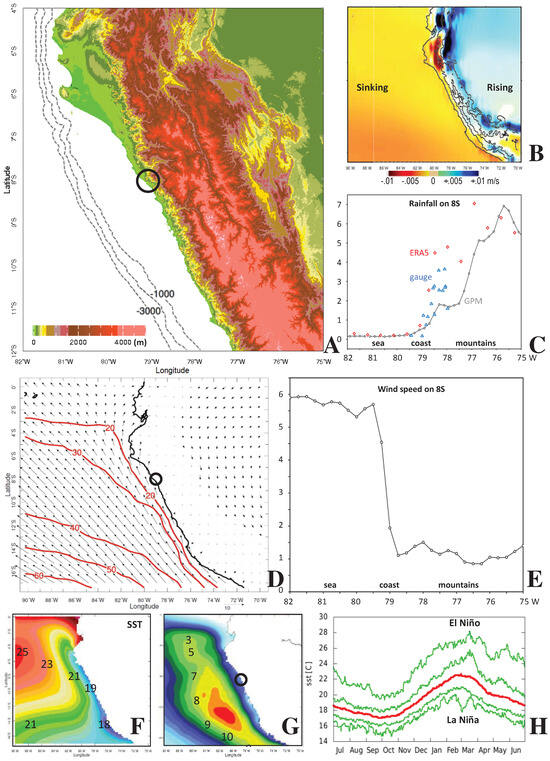
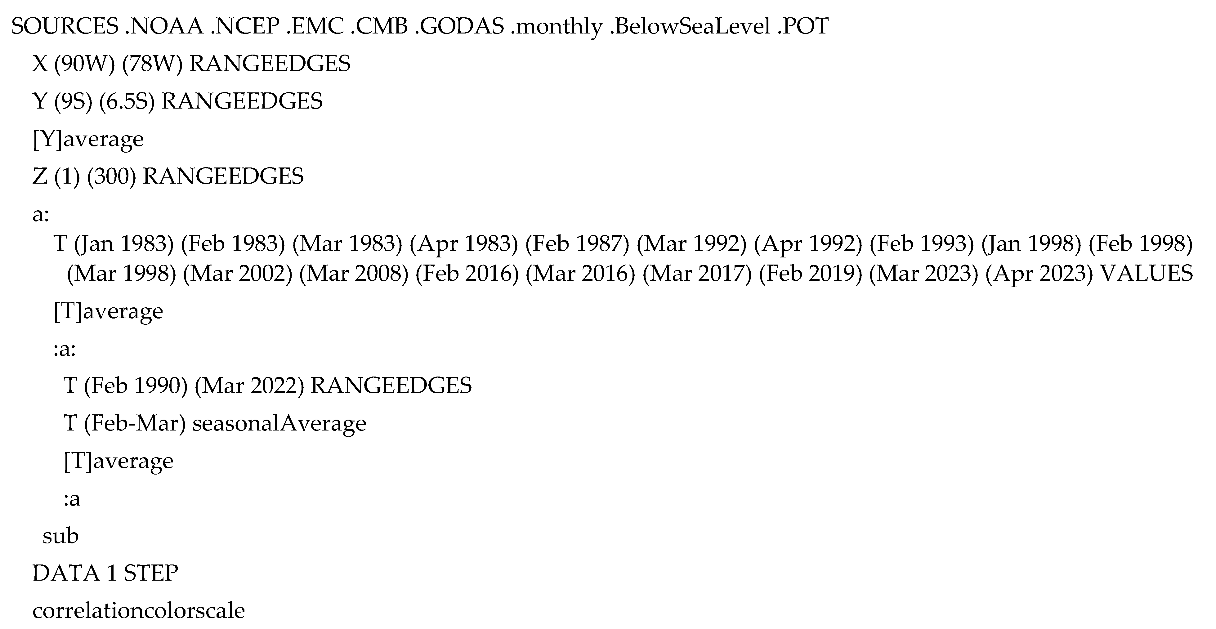
Figure 1.
(A) Topography (shaded)
and shelf edge (dashed) in the Moche area of Peru (o). Long-term
average: (B) vertical air motion at 700 hPa, (C) rainfall on 8S
slice: GPM (–o–), ERA5 ( ) and
gauges on the western slope (Δ), (D)
near-surface wind field (vector, largest 8 m/s) and ocean mixed layer depth
(red contours, m), (E) wind speed on 8S slice. Long-term SST analysis: (F)
average, (G) variance, (H) annual cycle in Moche area Peru (red
mean, green upper/lower quintiles), based on daily data 1979–2022.
) and
gauges on the western slope (Δ), (D)
near-surface wind field (vector, largest 8 m/s) and ocean mixed layer depth
(red contours, m), (E) wind speed on 8S slice. Long-term SST analysis: (F)
average, (G) variance, (H) annual cycle in Moche area Peru (red
mean, green upper/lower quintiles), based on daily data 1979–2022.
On the doorstep of northern Peru is the El Niño Southern Oscillation (ENSO), a leading source of global climate variability associated with tropical Pacific SST and trade winds [6]. ENSO’s warm and cool phases have opposing SST patterns whose eastward extent depends on ocean–atmosphere coupling in austral summer [7,8,9]. The tropical Atlantic and Indian Oceans show greater responses to eastern El Nino events [10], as does the wind-driven upwelling along the north coast of Peru. During neutral or La Nina conditions, the wind-driven upwelling persists, and the local weather remains sunny and dry. Past research has uncovered multi-decadal sequences of warm or cool ENSO phase [11], temporal shifts in ENSO transitions involving early or late onset [12], and north–south contrasts in Peru rainfall [13,14].
The arid north coast climate is punctuated by wet spells at quasi-decadal intervals which challenge resource management. Archeological evidence over five millennia has revealed an irrigation network to draw seasonal runoff from the western Andes for crop farming and socio-economic development [15]. Although floods occasionally led to destruction, hydraulic technology gradually improved so that late summer stream-flows could be converted to beneficial water supply. By the 15th century, indigenous communities were well established, but the equilibrium was upset by soil erosion/salinization and multi-decadal dry spells.
The east Pacific experiences a zonal tilting of the tropical thermocline accompanied by propagating ocean–atmosphere waves [16,17]. During eastern El Nino events such as in 1983 and 1998, Peru’s north coast receives an inflow of equatorial air [18,19]. Wind-driven upwelling ceases and SSTs increase above 26 °C, leading to atmospheric convection [20,21] at near-monthly intervals via eastward-moving Madden Julian Oscillations (MJO) [22]. A secondary process that affects the timing of local rainfall is the diurnal cycle [23]. Seabreeze convergence of humid air over the west-facing Andes as the coastal plains warm during mid-day. The subsiding southeasterly airflow turns shoreward and rises up-slope, so runoff tends to peak in the evening.
Local climatic features may be analyzed via modern numerical weather models underpinned by the global coupled data assimilation of satellite and in situ measurements. However, predictability is uncertain and impacts are problematic: flash-floods move quickly down the steep ravines, damaging hydraulic, agricultural and urban infrastructure, with knock-on effects for sediment transport, food and water shortages, and disease. In recent decades, flood events have become more frequent on the north coast of Peru. Whereas ancient society gained benefit from the runoff in the form of vegetation blooming events and replenished water supplies, modern society has lost some of that resilience—despite sophisticated warning systems that can distinguish the onset and extent of El Nino. Hence, our scientific questions include the following: (i) How does the coastal climate switch from stratiform to convective? (ii) Does the influence of coastal upwelling and ENSO shift N-S along the coast? (iii) Is the temporal character annually wet or infrequently wet? (iv) Are regional drivers of coastal warm events consistent with recent studies? (v) How can El Nino risks be better managed to sustain food and water resources?
2. Data and Methods
Along Peru’s north coast, 4–12S, 82–75W (Figure 1A), are the Chicama and Moche river-mouths and the city of Trujillo (8S, 79W), a center of pre-Columbian culture whose meso-climate was studied via hourly to monthly gridded satellite reanalysis products in the period 1979–2023. Our main focus is on river discharge, near-shore SST and winds, and potential evaporation (heat flux causing soil moisture depletion, [24,25]. Dataset acronyms, characteristics, and documentation are listed in Table 1. The reader should note that Peru’s national weather and ocean services make routine surface observations for assimilation in global models. These include a network of weather stations, hydrological streamflow, tide gauges, and in situ ocean variables from buoys and ships; however, upper air observations are scarce and necessitate satellite remote sensing.

Table 1.
Dataset details, characteristics, and references; coverage 1979–2023 unless indicated (yr+).
The discharge of the Chicama and Moche Rivers in the study area was derived by an EC hydrological model assimilation of daily in situ catchment rainfall and stream-flow measurements. To describe the weather and climate, ERA5 and CFS2 fields were analyzed for air pressure, wind velocity, vertical motion, temperature, specific humidity, potential evaporation, and convective available potential energy (CAPE). Rainfall (GPM) and sea surface height were derived from multi-satellite + gauge merged products, and coupled ensemble model forecasts were obtained. Moist convection was quantified by satellite net outgoing longwave radiation (OLR), and land temperature and vegetation conditions were analyzed via de-clouded satellite IR and VIS data (NDVI). Ocean reanalyses were employed to describe near-surface currents, vertical motion, temperature, and salinity along the north coast of Peru. Station records were derived from Trujillo airport hourly observations (8S, 79W) and daily tide gauge measurements at 4S, 8S, and 12S.
Time series of daily river discharge, SST, and meridional (V) wind were constructed for the Moche area (8S, 79W ± 0.25°) on the north coast of Peru (cf. Figure A1). The 44-year record of daily data (N = 44 × 365 = 16,070) was analyzed for long-term average, mean annual cycle, and extreme dry and wet cases: 14 October 2011 and 10 March 2023, respectively. The daily time series were lag-correlated across the entire record, 1979–2022, and per month (N = 1340) to establish the seasonality of wind-driven upwelling and hydrological response. Intra-seasonal pulsing was evaluated by 20–60-day band-filtering and wavelet spectral analysis.
Reducing these time series to monthly resolution, dry and wet groups were identified (Table 2) according to highest potential evaporation (dry early summer) and highest river discharge (wet late summer) for the subsequent composite analysis of regional anomalies of SST, wind, humidity (30S–15N, 150–30W), and subsurface ocean conditions over the Peru shelf (90–78W, 0–300 m). Anomalies were calculated by subtracting long-term mean October–November (dry) and February–March (wet) values. In addition, dry and wet composites of the atmospheric circulation were analyzed.
Table 2.
Based on time series in the Moche area, Trujillo, Peru, in chronological order: (a) dry months according to highest potential evaporation and (b) wet months according to highest river discharge. Rainfall (mm/day) or discharge (m3/s) and SST (°C) also given. These groups are used to form composites: Figures 5, 6, 8 and 9.
The river discharge time-series was point-to-field regressed onto fields of runoff and net OLR to quantify spatial decorrelation and define a zone of ‘sympathetic’ climate responses and impacts within the area 0–17S, 90–70W. Independently, a Principal Component analysis of evapotranspiration (ERA5 latent heat flux) and satellite vegetation NDVI was conducted to determine areas with similar mean annual cycle and response to eastern Pacific ENSO. These support the use of the Moche area time series as an indicator of climate variability on the north coast of Peru.
The January–March river discharge was analyzed for inter-annual ocean–atmosphere teleconnections by point-to-field correlation with Hadley SST [34], satellite OLR, and 850 hPa zonal wind. The 1979–2022 records have ~44 degrees of freedom due to annual cycling, so 95% confidence is reached with |R| > 0.30. Lag correlations were calculated between the Moche area discharge/pot. evap. and the Pacific ENSO variables: SST in prescribed areas Nino1–2, Nino3, and Nino4, the multi-variate ENSO index MEI2, and Pacific Decadal Oscillation PDO.
Among the methods, the point-to-field correlation maps use all 44 seasons to establish standardized, linearly opposed spatial patterns that tend to be dominated by the larger ± ENSO events. In contrast, the composite technique separates dry early summer and wet late summer, uses ~15% of the total months, and assigns equal weights therein. These statistical approaches will generate different outcomes.
Mean diurnal cycles in the Moche area were analyzed using hourly time series of GPM rainfall and zonal (U) wind during late summer wet spells in December 2014–April 2015 and December 2022–April 2023. Departures from the all-hour mean were analyzed for MERRA2 11:00–14:00 surface temperatures, with 14:00–17:00 wind velocity and 17:00–20:00 GPM rainfall over the 0–17S, 90–70W area. This helps to establish the link between afternoon sea breezes and evening flash floods.
The wet spell in March 2023 was analyzed for airflow patterns, SST, and ocean currents, and the daily time series of GPM rainfall and sea surface height. This outcome shows an influx of equatorial air over high SST that may be compared with an earlier El Niño wet spell in March 2017.
To evaluate long-lead forecasts, the EC ensemble model for Jan, Feb, Mar rainfall hindcasts and 3-month forecasts for 1980–2017 were compared. Although the EC model corresponds with GPM-gauge observations at the coast, it has a wet bias over the Andes. A further statistical limitation is the small degrees of freedom owing to the infrequent nature of floods. Short-term forecasts were evaluated via the CFS2 ensemble model for daily rainfall hindcasts and 1-month forecasts for 2014–2022. The linear regression fit is the primary measure of skill, which for daily data was restricted to rainfall > 0.1 mm.
The workflow progresses from mean climate and cross-coast gradients to environmental conditions in dry early summer and wet late summer. Tropical late summer rainfall over Andes catchments is beneficial except when amplified to flood proportions by El Nino conditions, as the statistics demonstrate. Lag-correlations enable inferences on how central Pacific warm events spread eastward with coupled ocean–atmosphere Kelvin waves.
3. Results
3.1. North Coast Climate and Seasonality
The geography (Figure 1A) of the Moche area shows a straight NNW coastline backed by steep mountains that separate atmospheric sinking and rising motions (Figure 1B), resulting in a sharp eastward increase in orographic rainfall on 8S (Figure 1C). The shelf is broad and overlain by shallow equatorward winds (Figure 1D) aligned to the coastal plains. The prevailing SSE winds at Trujillo airport (Figure A2) are rarely outside that sector. Marine winds of ~6 m/s decrease rapidly at the coast (Figure 1E), leaving a shallow mixed layer and imparting cyclonic vorticity (−10−4 s−1) that enhances near-shore upwelling. Long-term mean SST (Figure 1F) exhibits upwelling effects <20 °C in a plume that extends along the coast ~200 km wide of the Moche area, narrowing equatorward/widening poleward. The mean annual cycle of SST (Figure 1G) reaches a minimum/maximum in September–October/February–March, a few months behind the atmospheric heat budget. Upper/lower quintiles of SST depend on La Nina/El Nino influence and range from 18 °C to 26 °C in late summer. A circular area of tropical SST > 25 °C~6S, 90W often reaches the shelf edge, causing high SST variance there (Figure 1H).
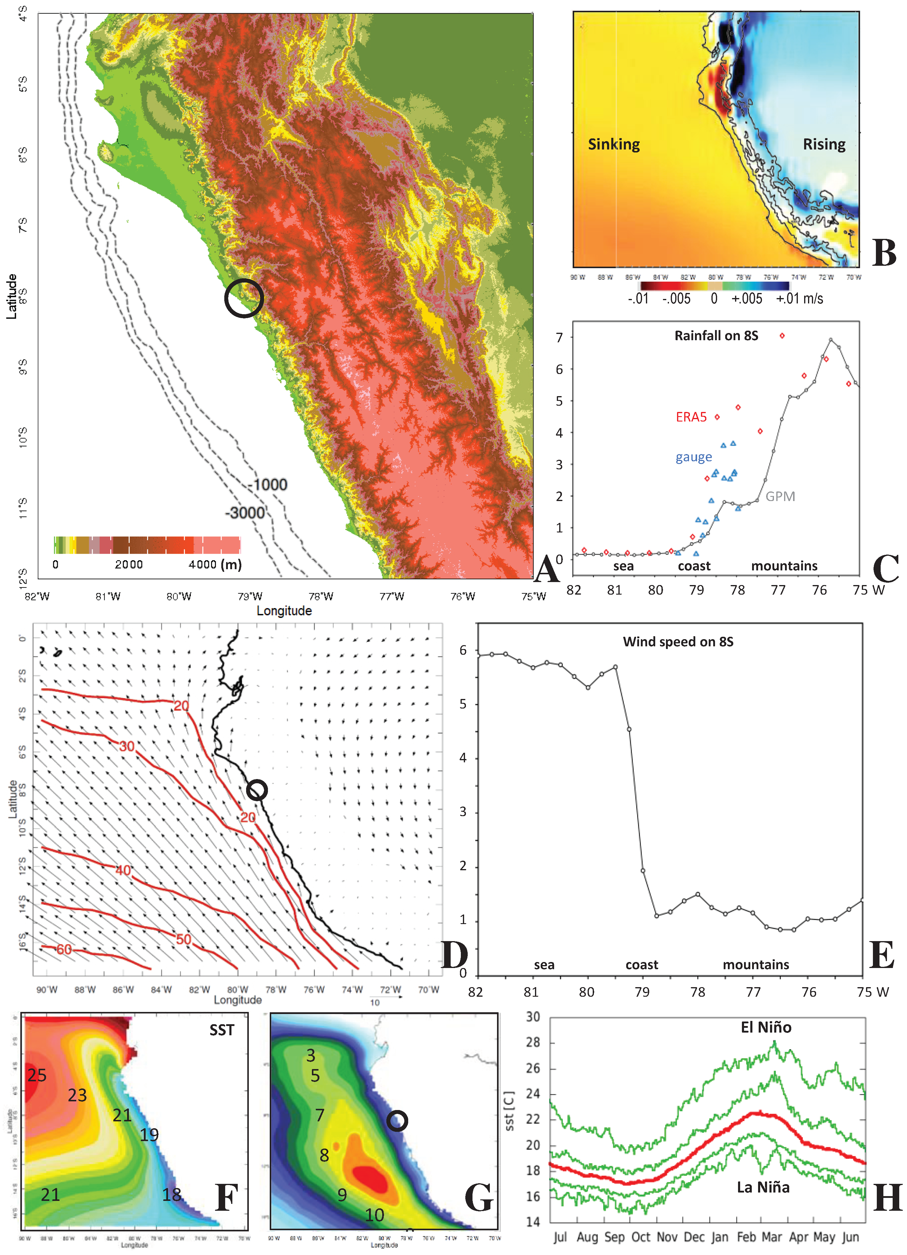
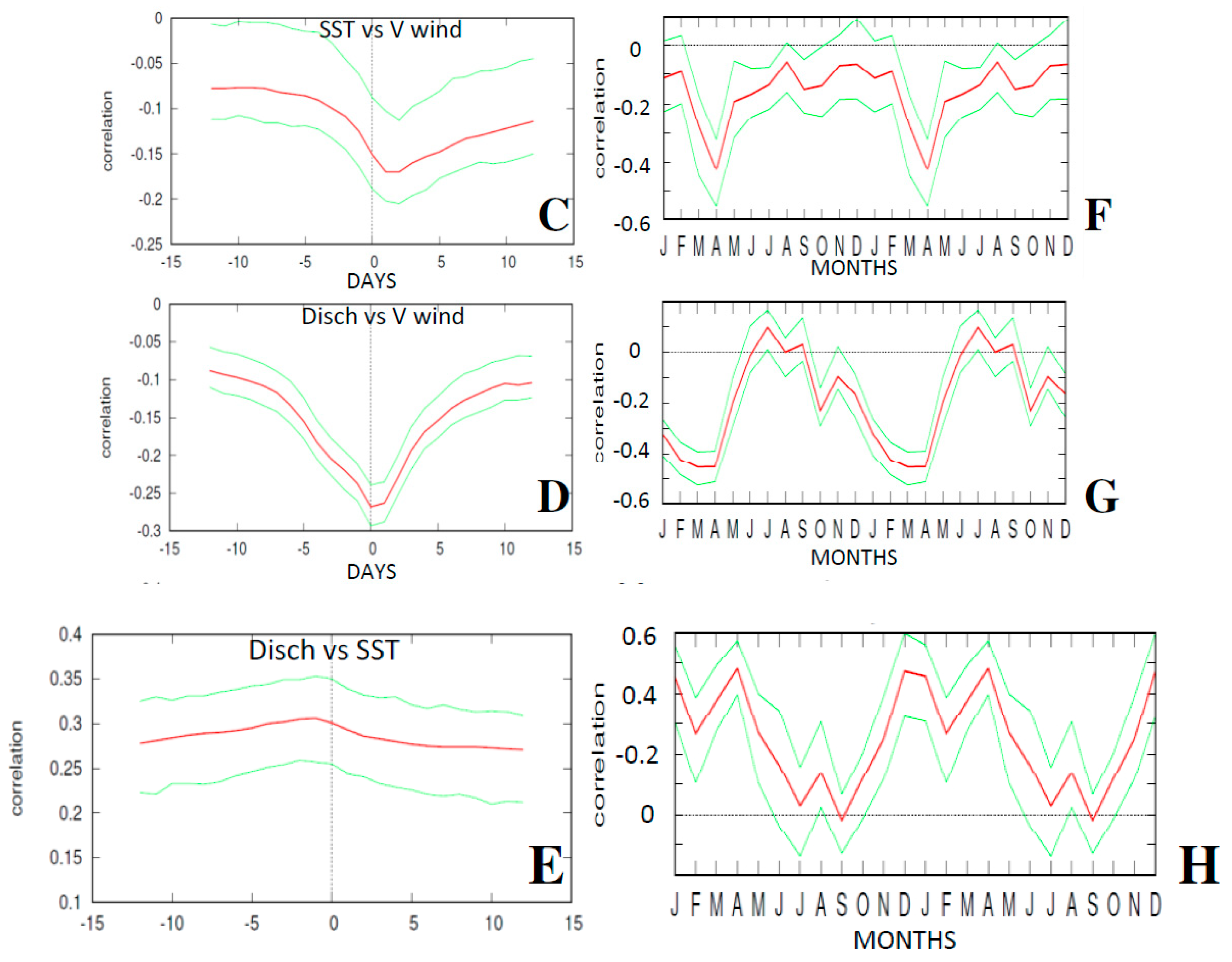
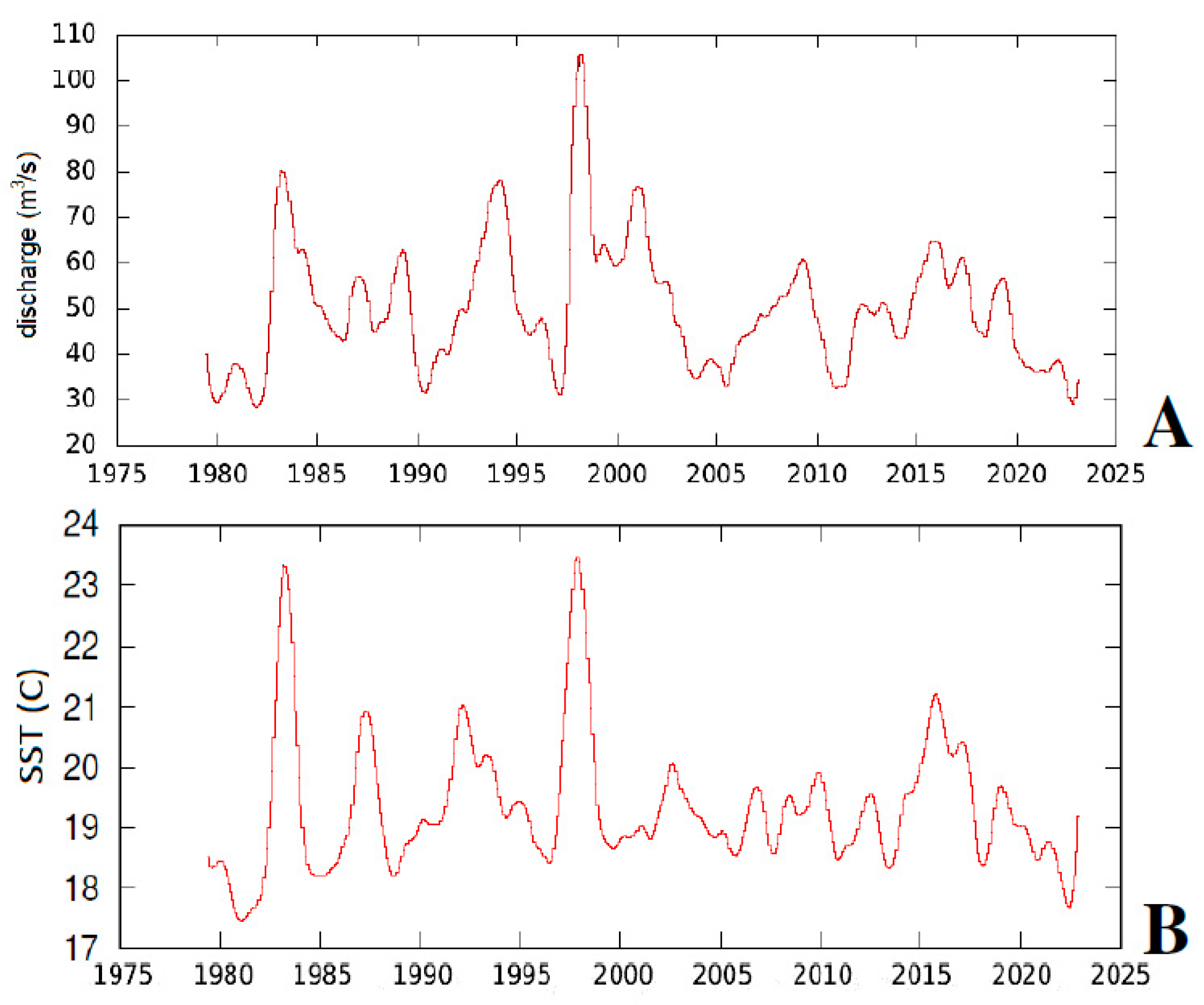
Turning our attention to the Moche area hydrology, Figure 2A shows the daily river discharge over the 44 yr record, with an annual rhythm aligned to SST. Intra-seasonal oscillations tend to occur at monthly interval, according to wavelet spectral analysis (Figure 2B). Wind-driven upwelling suppresses river discharge, as seen in lag correlation and monthly plots (Figure 2C–H). Equatorward winds tend to cool SST a day later, but correlations are weak (R~−0.15) except in March–April (−0.4), indicating secondary effects from net heat flux and current advection. Relationships with discharge are informative: a reduction in equatorward winds contributes to a rapid increase in river flow (R~−0.25) that is particularly strong in February–April (−0.45). SST naturally exhibits a more gradual influence on discharge (R~0.30) from −3 to +2 days. Correlations per month show a double maxima (R > 0.4) in November–December and March–April when local weather couples with anomalous ocean conditions.
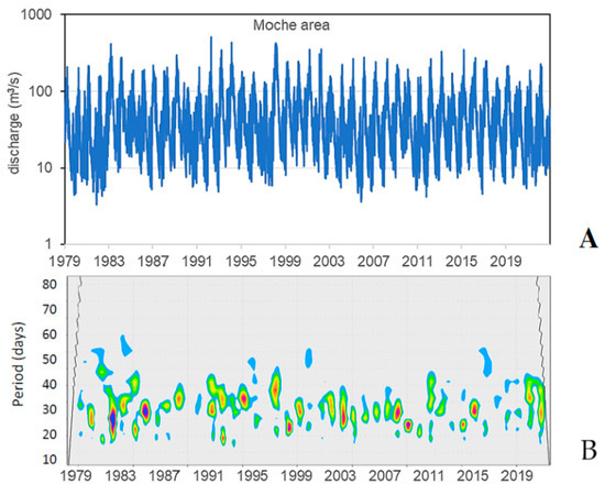
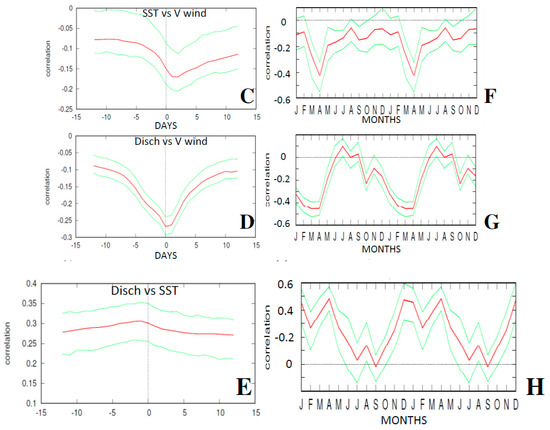
Figure 2.
(A,B) Moche area daily fluvial discharge and its spectral power after 20–60-day band-filtering, shaded blue to red for 90 to 99% confidence. Lag correlation between continuous daily time series in the Moche area, Trujillo, Peru: (C) SST vs. V wind, (D) discharge vs. V wind, (E) discharge vs. SST. Correlation between the same time series but segregated by month: (F) SST vs. V wind (1 day earlier), (G) discharge vs. V wind (0 lag), (H) Moche discharge vs. SST (0 lag) and duplicated to reflect austral summer. In (C–H) red line is mean, green lines are 95% confidence intervals.
The inter-annual filtered time series of Moche area discharge and SST (Figure 3A,B) are linked through the ENSO phase. The local SST leads discharge by 2–4 months (R > 0.6) and both exhibit 2–8 yr cycles that are strong before 2000 and weak thereafter. To check for coherence between Moche area discharge and the north coast climate, point-to-field correlations were calculated with respect to runoff and net OLR (Figure 3C,D). Sympathetic values spread along the west-facing Andes from 0 to 17S, and into the equatorial east Pacific. Runoff derives from rainfall on the western slopes of the Andes mountains (not snowmelt). The spatial correlation map suggests that the Moche area discharge can be used to indicate ENSO-modulated climate forcing across the region.
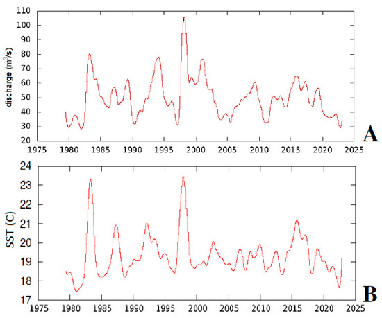
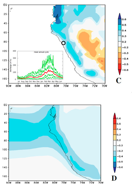
Figure 3.
(A,B) Time series of inter-annual filtered Moche river discharge and coastal SST. Correlation of Moche area river discharge (8S, 79W) with January–March 1979–2022 fields of (C) surface runoff and (D) net OLR; blue shading is wet and outlines the coherent zone. Inset in (C) is the mean annual cycle of daily Moche area fluvial discharge and upper/lower quintiles.
3.2. Regional Teleconnections
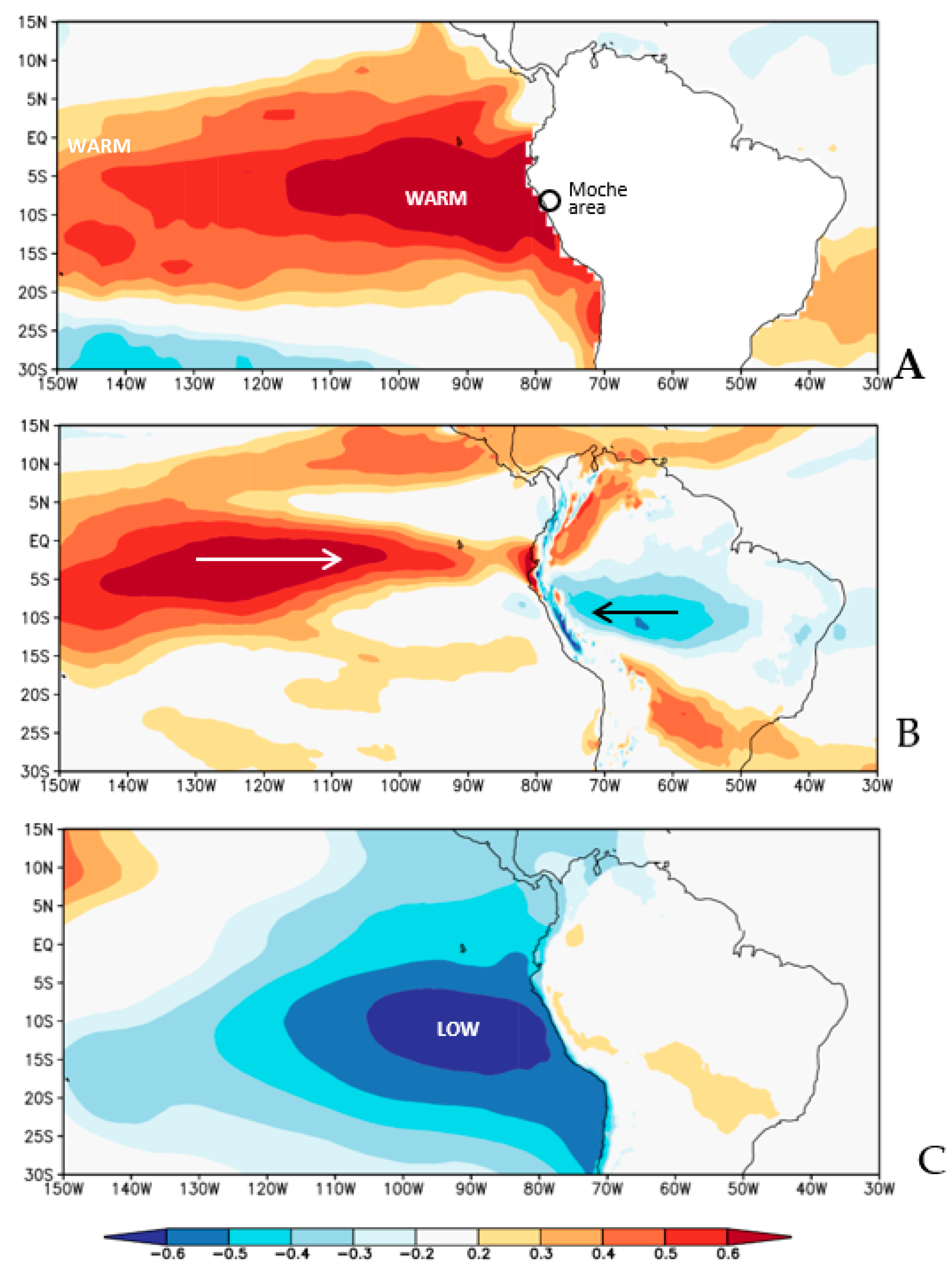
Point-to-field correlations between the January–March discharge time series and SST, 850 U wind and surface air pressure fields are illustrated in Figure 4A–C. Moche rivers flow when the tropical Pacific SST exhibits an eastern El Nino warming (5–10S, 140–80W) coupled with westerly winds (0–5S, 150–90W) and a weakened SE Pacific anticyclone (10–15S, 110–80W). A secondary feature is easterly winds from the southern Amazon that push up against the Andes and ‘leak’ onto the Peruvian north coast at 6S. Table 3 confirms that Nino1–3 and MEI2 have significant influence on the January–March Moche area discharge. The influence of eastern and coastal ENSO forcing seems blurred; they act in concert, according to the broad extent of high correlations in Figure 4B. Table 3 also suggests that Nino4 and PDO had minimal influence on Moche area discharge in 1979–2022.

Figure 4.
Correlation with January–March fields of (A) SST, (B) 850 U wind, (C) SL. pressure, 1979–2022. Arrows in (B) refer to wind direction.
Table 3.
Correlation of January–March Moche river discharge with ENSO variables. Lead/lag months before/after; N = 44, 95% confidence at r > 0.30. Values are listed in descending order, with significant peaks underlined.
3.3. Dry Climate and Weather
The dry early summer composite satellite daytime land temperature and vegetation maps (Figure 5A,B) reveal that the coastal plains are warm ~40 °C and sparsely covered (green fraction < 0.2), due to sinking motions imparted by divergent anticyclonic winds and cool SST in early summer. The principal component analysis of evapo-transpiration and vegetation (representing the Peruvian north coast) have mean annual cycles that follow SST: maxima in February–April/minima in September–November (Figure 5C). The terrestrial hydrology ‘turns off’ as wind-driven upwelling intensifies.
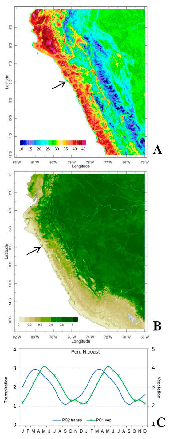
Figure 5.
Composite dry conditions based on months in Table 2a and high-resolution satellite data: (A) IR daytime land temperature and (B) VIS color fraction, with an arrow on the Moche area; map scales differ. (C) Mean annual cycles of evapo-transpiration (mm/day) and vegetation color (fraction) in the north coastal plains, duplicated to reflect austral summer.
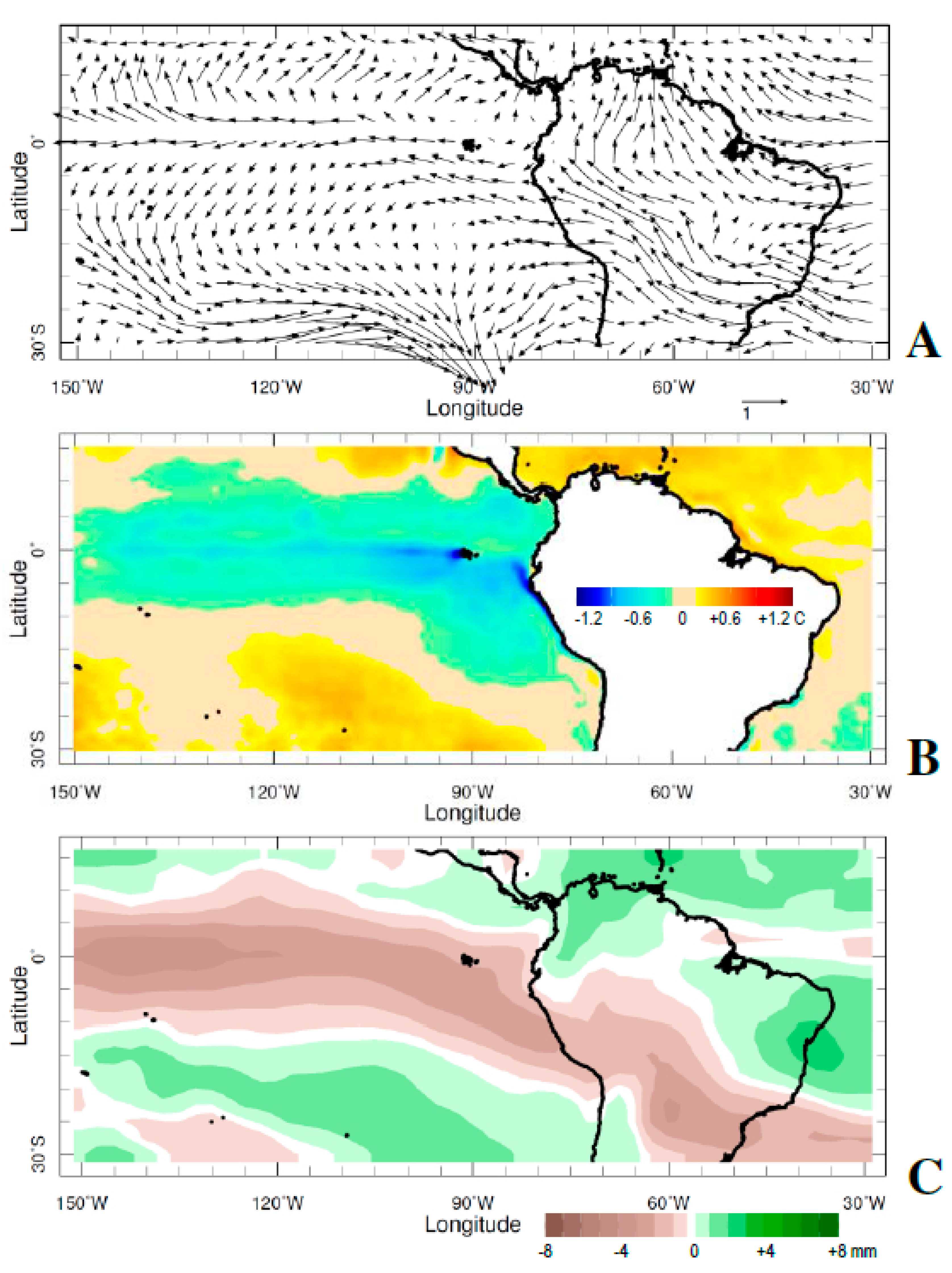
Dry composite climate anomalies (Figure 6A–C) based on months listed in Table 2a feature equatorial trade winds diverging away from an east Pacific cold tongue (SST anomaly < −1 °C). There is an axis of dry air extending from subtropical South America to the equatorial east Pacific (moisture anomalies −8 mm). A Rossby wave pattern focuses extra-tropical troughs and poleward airflow on 30S, 90W. These features tend to weaken eastward, moving ocean Kelvin waves in the equatorial Pacific, consistent with La Niña conditions.

Figure 6.
Dry composite anomalies: (A) 925–850 hPa winds, (B) SST, and (C) precipitable water, based on ERA5 reanalysis and months listed in Table 2a.
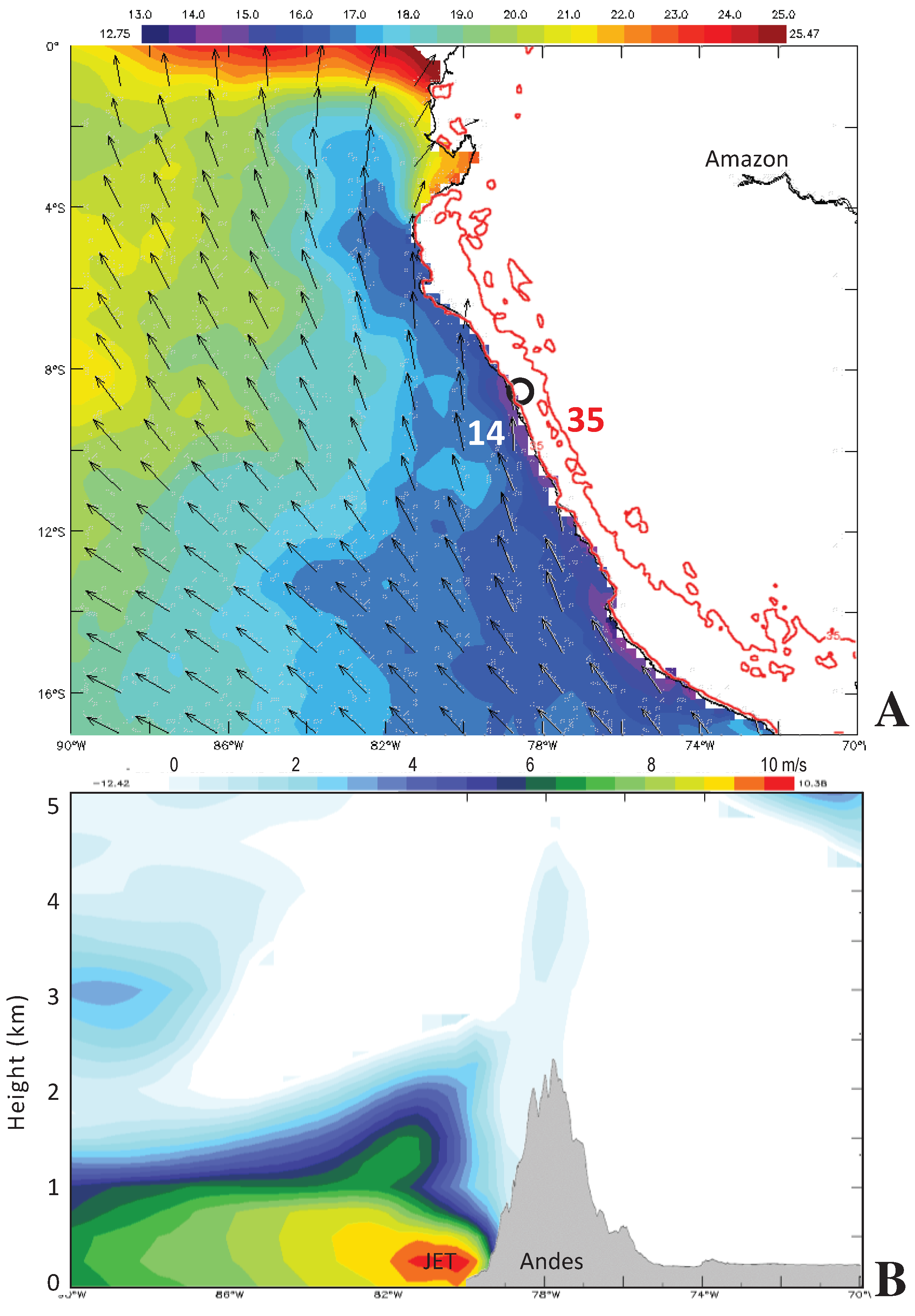
A spell of dry weather on 14 October 2011 is analyzed in Figure 7A,B. Wind-driven upwelling cooled SST over the shelf to 14 °C. A low-level equatorward wind jet of 10 m/s accelerated along the coast, while daytime temperatures on the coastal plain exceeded 35 °C. The Hadley circulation was displaced northward, thereby damping equatorial ocean Kelvin waves. River discharge in early summer tends to stay below 10 m3/s.
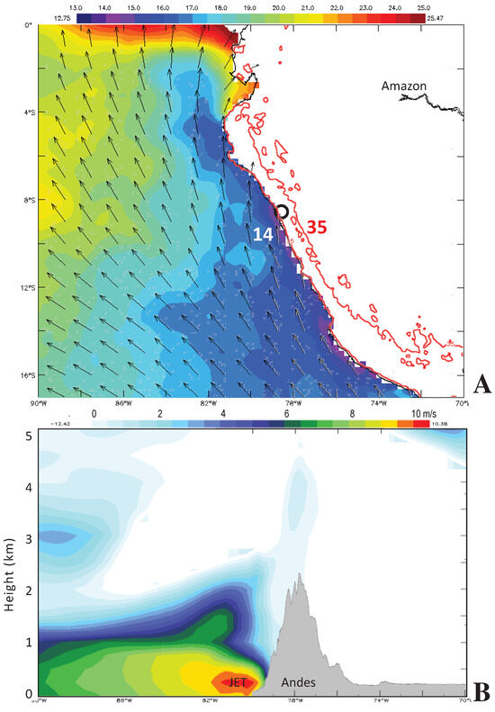
Figure 7.
(A) Marine winds (vector) and SST (shaded) and max land temp > 35 °C (contour), (B) W–E height section 6.5–9S of the equatorward wind jet, during a dry spell and upwelling event on 14 October 2011.
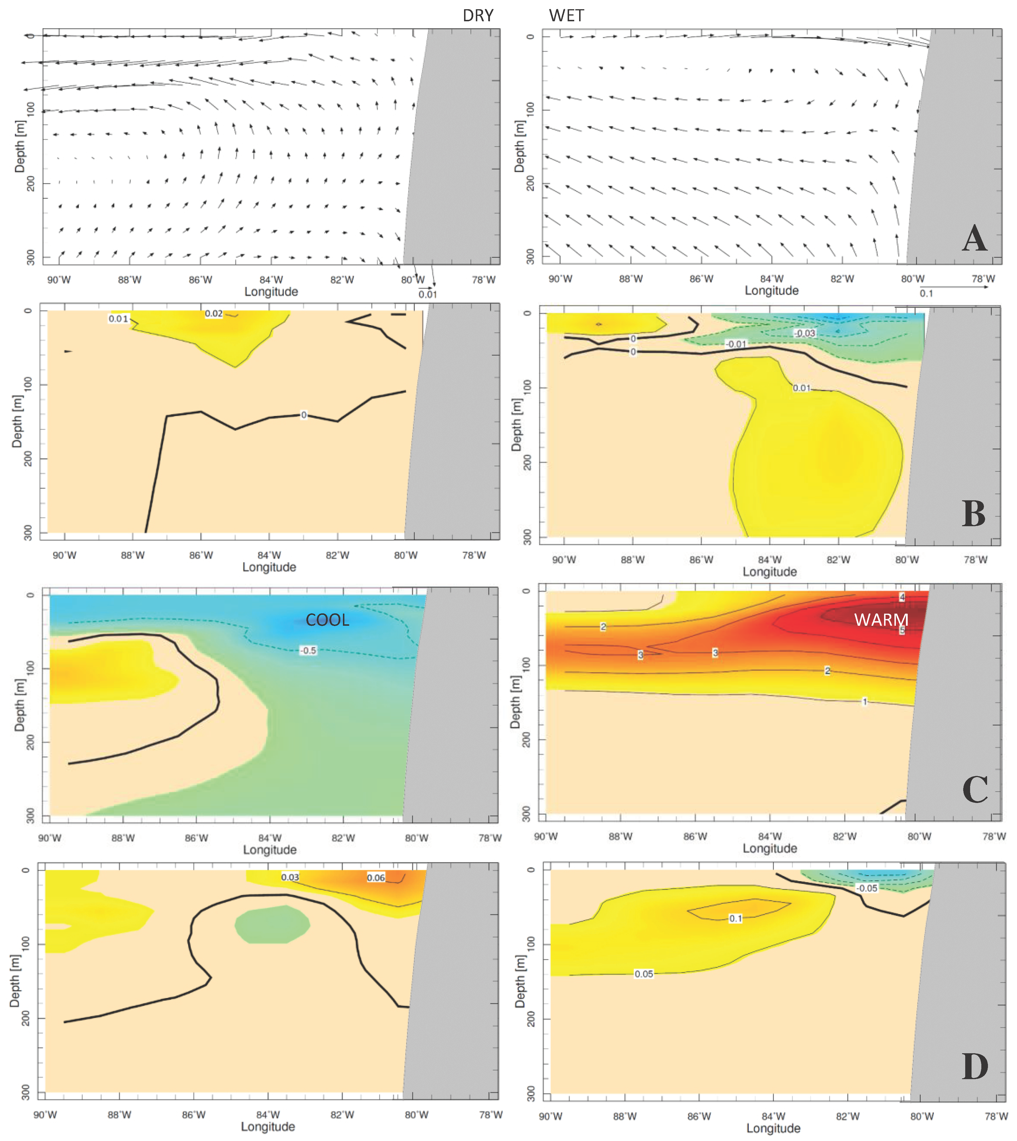
3.4. Shelf Composites: Dry vs. Wet
In this section, we employ GODAS ocean data over the shelf of northern Peru (averaged 6.5–9S) to contrast dry and wet composite anomalies, based on the months listed in Table 2a,b. The opposing patterns exhibit asymmetry in Figure 8A–H. The dry composite has offshore Ekman transport, near-shore upwelling, and northward currents, whereas the wet composite shows onshore transport, downwelling, and stronger southward currents. Near-shore upper ocean sea temperature anomalies are −1 °C in the dry composite, but +4 °C in the wet composite. Salinity reflects near-shore negative anomalies in wet climate due to rainfall and runoff. It is noted that quarterly ship sections at various latitudes over the shelf [40] underpin the model-interpolated results.

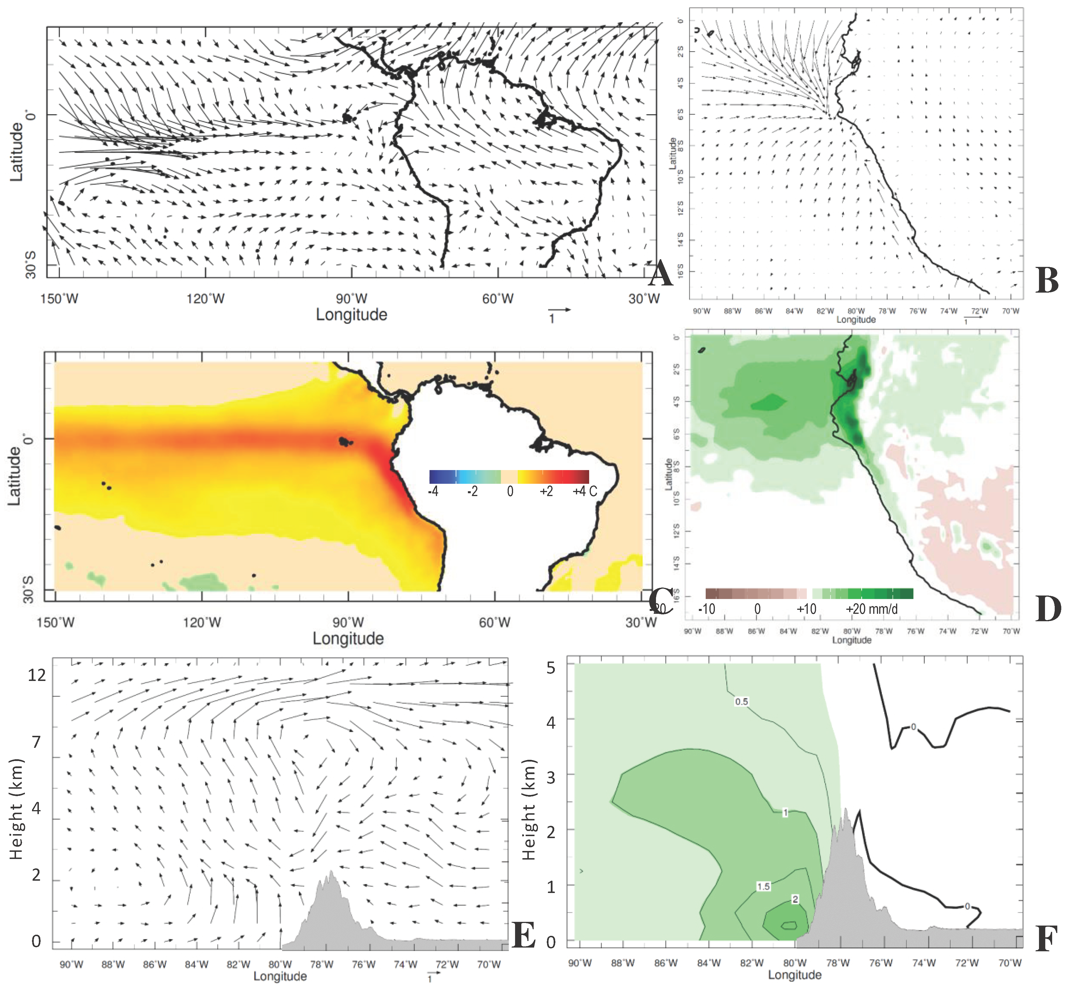
3.5. Wet Composite
In this section, we focus on wet composites using months listed in Table 2b. Figure 9A,C present regional maps, while Figure 9D–F illustrate local features. Low-level westerly wind anomalies flow across the equatorial east Pacific (10N–10S, 150–80W) toward Ecuador, where they divide. Low-level wind anomalies over the Amazon turn northward into the Caribbean. SST anomalies are +4 °C above normal off Peru and in the equatorial east Pacific (Nino1–3). Surface wind anomalies are northwesterly and confluent near 4S, 82W, where rainfall anomalies are >+10 mm/day. The wet conditions extend from Ecuador along the Peruvian north coastal plains. The wet composite height sections reveal an anomalous zonal overturning circulation: it is upper eastward/lower westward, sinking to east/rising to west of the Andes (Figure 9E). This represents a mini-Walker cell driving El Nino-induced late summer wet spells. Warm SST and rising motions generate a core of anomalous humidity over the shelf (Figure 9F).
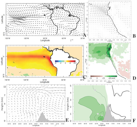
Figure 9.
Wet composite anomalies: (A) 925–850 hPa wind, (B) local 1000 hPa wind, (C) satellite SST, (D) local rainfall. Wet composite anomaly W–E height section averaged over 6.5–9S of (E) zonal circulation wind vectors to 12 km and (F) specific humidity to 5 km with topographic profile, based on ERA5 reanalysis and months listed in Table 2b. A ‘mini-Walker Cell’ is located over the Andes during wet spells.
3.6. Diurnal Cycling
Diurnal cycles in local rainfall and surface zonal winds are studied using hourly satellite reanalysis data during December–April wet spells for 2014–2015 and 2022–2023. Both time series, when averaged by hour, exhibit afternoon peaks (Figure 10A–D). Values are near zero all night and in the morning, and then as winds shift to westerly ~2 m/s by 12:00 h, rainfall increases >0.3 mm/h by 15:00 h. Outliers are uniform and symmetric for wind but tend to peak~0.8 mm/h for afternoon rain. Maps of mean surface temperature, wind, and rainfall departures for successive 3 h periods (Figure 10E–G) demonstrate how the heating of the coastal plains triggers onshore sea-breezes and afternoon rainfall over the west-facing Andes. An inspection of wind departures indicates that coastal sea-breezes draw warm, humid air from the northern shelf. Thermal gradients (+10C/100 km) converge airflow onto the Andes, thereby stimulating atmospheric convection and flash floods in the evening.
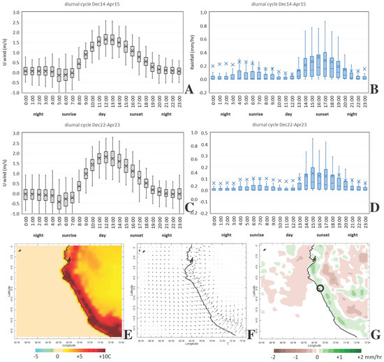
Figure 10.
Mean diurnal cycle box-whisker plots of Moche area ERA5 zonal wind and GPM hourly rainfall in wet seasons: (A,B) December–April 2015, (C,D) December–April 2023. Maps of diurnal departure from overall mean: (E) surface temperature 11:00–14:00 h, (F) surface wind 14:00–17:00 h (largest vector 3 m/s), and (G) rainfall 17:00–20:00 h (local time), based on hourly December–April 2023 data, N = 150.
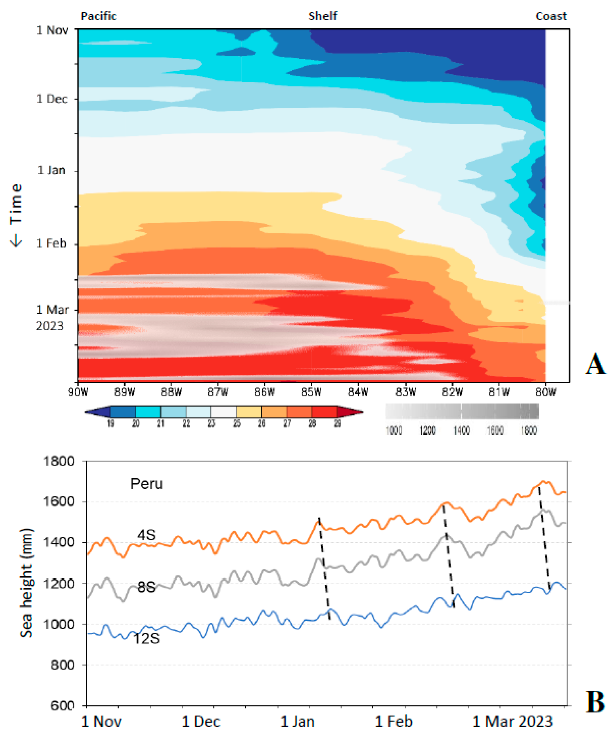
3.7. Late Summer Wet Spell, 2023
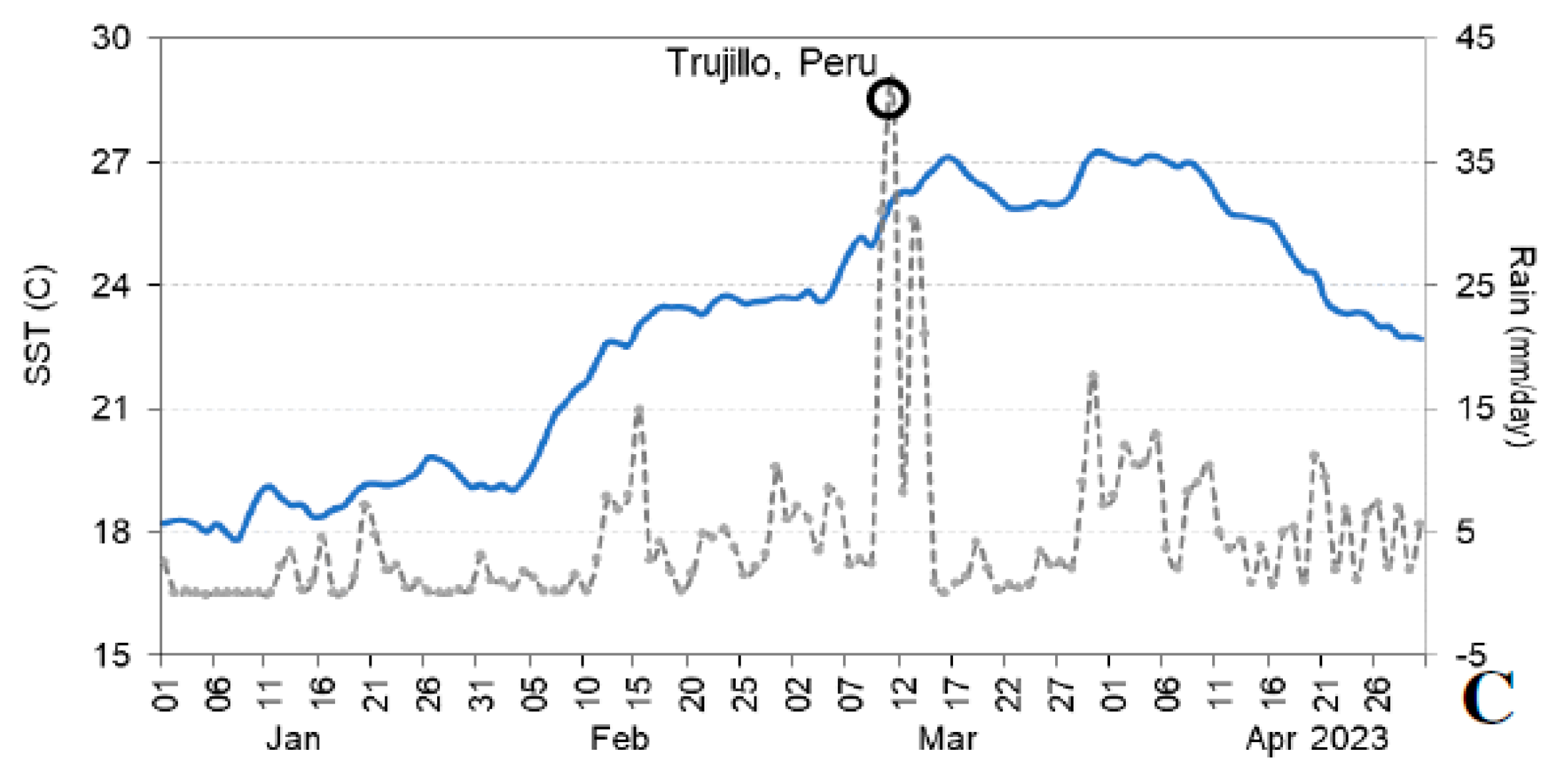
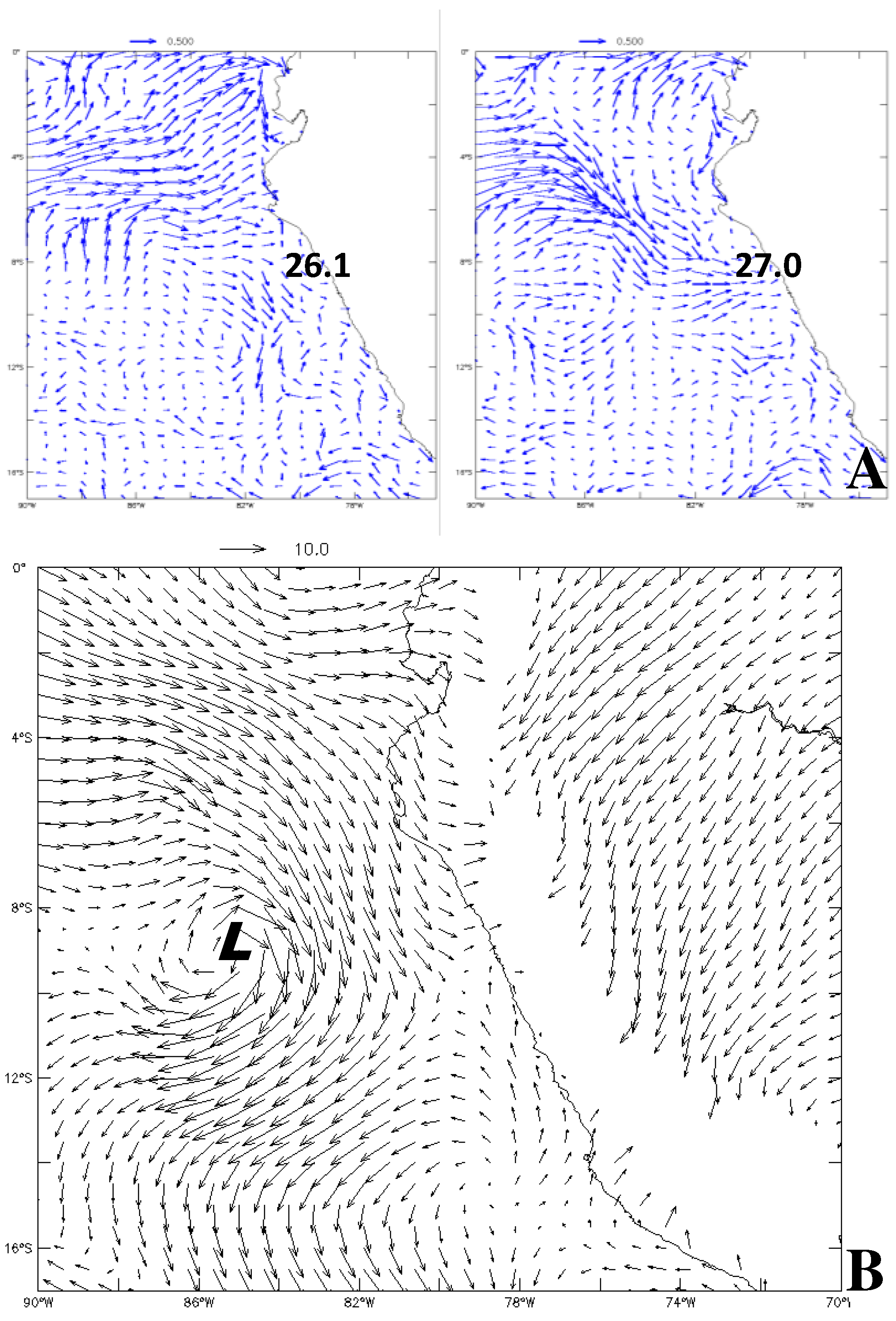
In this section, an El Nino-induced wet spell in northern Peru is studied via Hovmöller analysis of SST and CAPE on 8S (Figure 11A). Early summer (November 2022) saw wind-driven upwelling, cool SST < 19 °C, and dry weather. SSTs started warming in January 2023 as winds relaxed, and then continued >28 °C in February–March 2023 pulsing CAPE > 1500 J/kg. Sea height time series (Figure 11B) from gauge measurements exhibited a gradual rise punctuated by three surges, moving poleward along the coast at ~2.3 m/s. This phase speed was consistent with domes of warm seawater carried by ocean Kelvin waves [41] accompanied by northwest winds, onshore Ekman transport, and downwelling. Time series of daily SST and rainfall (Figure 11C) exhibited three upward steps in early February, March, and April. Heavy rainfall on 10–12 March was driven by an inflow from the equatorial Pacific. Figure 12A,B show maps of currents and winds that indicate a build-up of southeastward currents 0.5 m/s over the shelf induced by a quasi-stationary low pressure cell (cyclone Yaku) at 9S, 87W.
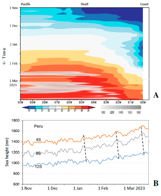
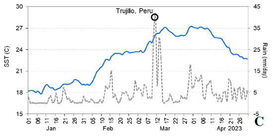
Figure 11.
El Niño flood: (A) Hovmöller plot on 8S of daily SST (color shaded) and CAPE (gray shaded > 1000 J/kg) across the shelf, November 2022–March 2023. (B) Daily measurements of sea level at 3 places along the north coast of Peru, November 2022–March 2023, with dashed lines highlighting poleward signals. (C) Time series of SST (blue line) and rainfall (dashed grey line) at Trujillo in January–April 2023.
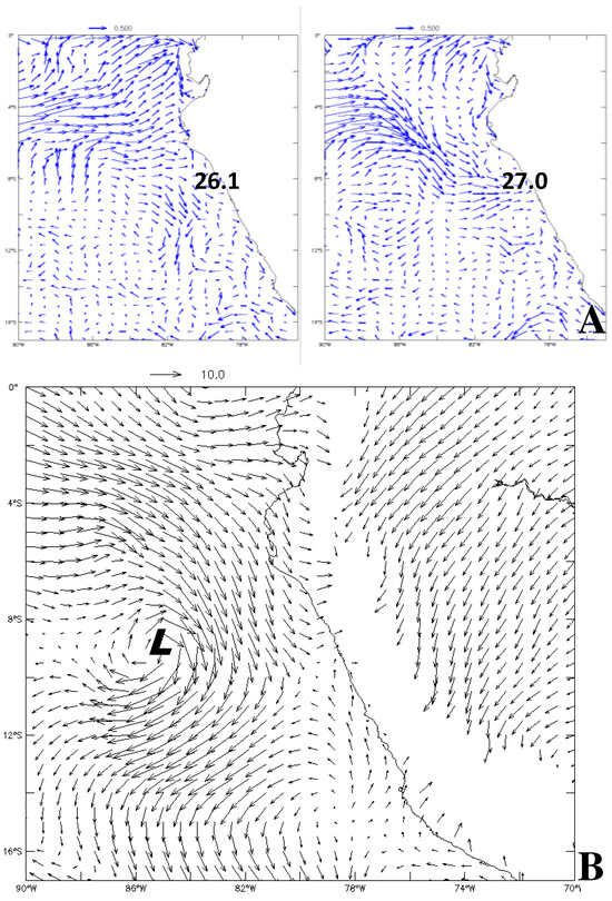
Figure 12.
El Niño flood: (A) HYCOM3 surface currents: 11 (left) and 15 March 2023 with Moche SST labeled. (B) Map of 850 hPa wind during the wet spell, 10 March 2023. The marine low persisted for many days. Currents (blue) and winds (black) are represented as vectors according to arrow size.
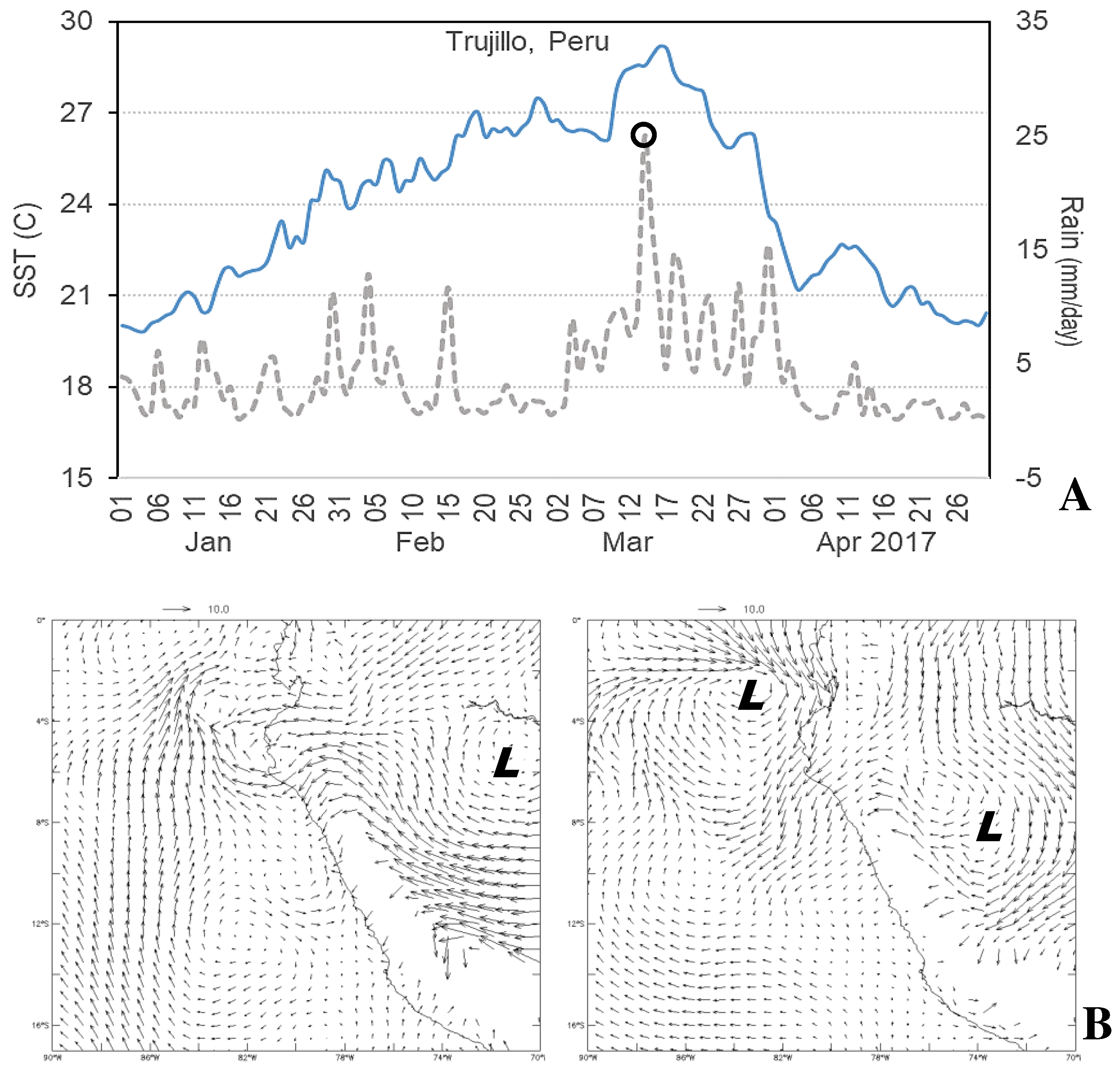
Comparing the March 2023 wet spell with March 2017 [21,40], we find that coastal SST warmed rapidly after January and reached 29 °C by March (Figure 13A). Heavy rains on 14 March 2017 were supported by moist inflow from the east (Figure 13B) and cyclonic vortices over eastern Peru and Ecuador. The coastal El Nino caused humid Amazon air to spill across the Andes. Both events show a gradual increase in poleward airflow that is pulsed by ocean–atmosphere coupling.
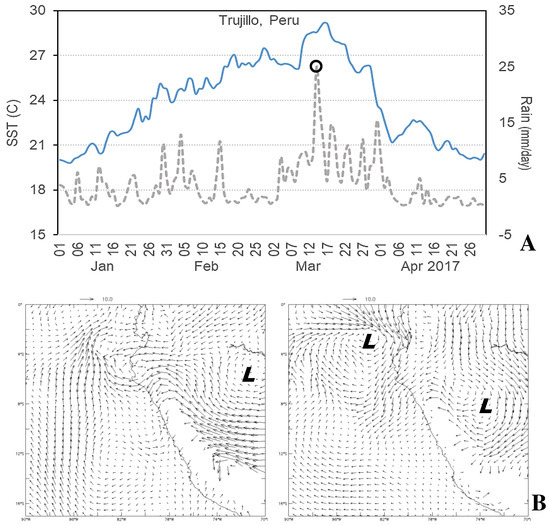
Figure 13.
(A) Time series of daily SST and rainfall at Trujillo, January–April 2017; (B) maps of 700 hPa wind during the El Niño flood: 14 March 2017 (00Z left, 18Z right), indicating rapid formation of a marine low west of Ecuador. Blue lines indicate the atmospheric inflow.
3.8. Long-Lead Forecasts of Monthly and Daily Rainfall
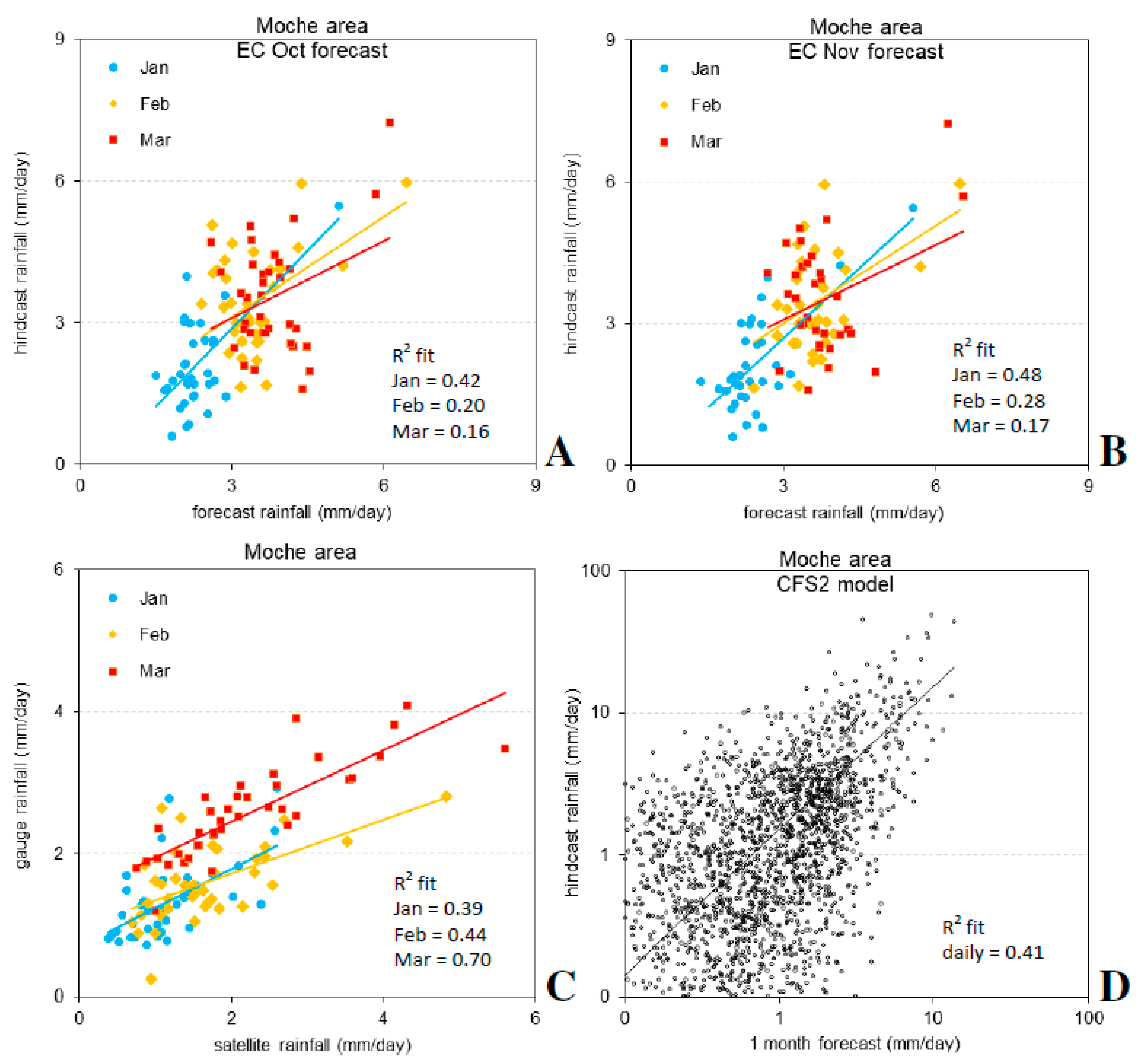
Here, we evaluate coupled ensemble model forecasts from the ECMWF and CFS2 models for the Moche area. Oct and Nov forecasts for late summer (Figure 14A,B) show best fit with the Jan rainfall (R2 0.42–0.48), thereafter declining to 0.16–0.28 for February–March rainfall. November forecasts are only ~5% better than October, and seasonal forecasts barely exceed ‘chance’. We question why February–March forecasts are poor at one-season lead, given the well-documented ocean–atmosphere coupling. A larger target could improve hit-rates but would mix mountain and marine regimes. The low forecast skill may relate to weak La Nina signals and to different atmospheric Walker circulations in central (standing) vs. eastern (transient) ENSO [42].

Figure 14.
Moche area rainfall evaluation: (A,B) ECMWF October and November forecast compared with the January, February, March hindcast, (C) IR-satellite compared with gauge rainfall for January, February, March 1982–2020, (D) CFS2 daily rainfall one-month forecast compared with hindcast 2014–2022 (log-scale, zero values omitted), all with linear regression fit.
In contrast to forecasts that weaken over late summer, the statistical fit of the satellite to gauge rainfall improves from January to March (Figure 14C). Monthly GPM satellite rainfall exhibits a low bias in dry spells but matches during wet spells, with little dispersion in March (R2 0.70). Daily rainfall forecasts by CFS2 at the 1-month lead (Figure 14D) show moderate skill (R2 0.41), with dispersion below 5 mm/day. At higher rain rates, the daily forecasts are better, albeit with a dry bias over the period 2014–2023.
4. Concluding Discussion
Climate variability on the north coast of Peru has been studied using high-resolution satellite and model reanalysis. Wind-driven upwelling and atmospheric subsidence prevail, except for a couple of wet months in late summer. Long-term averages reflect sharp zonal gradients in SSE wind and rainfall across the coast. Statistical composite analysis and point-to-field regression provide useful insights, based on monthly river discharge and potential evaporation time series for 1979–2023 in the Moche area (8S, 79W). Dry early-summer composites had divergent airflow over the east Pacific cold tongue. As the southeast Pacific anticyclone expands, an equatorward longshore wind jet of ~10 m/s accelerates off northern Peru, and the equatorial trough shifts to 10N. In contrast, high river discharge corresponded with warm SST anomalies +4 °C accompanied by 0.5 m/s poleward currents, low salinity, and a shallow downwelling circulation. In the atmosphere, a mini-Walker cell was discovered (cf. Figure 9E). The wet composite featured upper-level westerly/low-level easterly wind anomalies that lift humid air over coastal SST ~27 °C.
In addition to multi-year climate variability, intra-seasonal oscillations were studied using daily data. Many days before flood events, sea levels rise off Ecuador and domes of warm water spread poleward along the north coast of Peru. These ocean Kelvin waves are characterized by a 6000 km length, 2.3 m/s phase speed, and ~30-day cycle that corresponds with the pulsing of rivers during austral summers under the influence of warm-phase ENSO [43]. In contrast, cold-phase conditions suppress the coupling and propagation of zonal waves into the equatorial east Pacific.
Atmospheric convection was found to be concentrated by the diurnal cycle. Hourly data showed the 10 °C heating of Peru’s north coastal plains at midday, followed by an onshore airflow of 3 m/s that lifts over the west-facing Andes, generating mean diurnal rainfall ~1 mm/h near sunset. Wet spells in March 2023 were analyzed for synoptic weather forcing. A quasi-stationary low pressure cell formed off the north coast over SST > 28 °C. Southeastward surface currents and airflow increased CAPE > 1500 J/kg, leading to heavy rainfall on the evening of 10 March 2023. East Pacific El Ninos, such as in March 2017, drive coastal SST up to 29 °C and cause humid air from the Amazon to spill over the Andes mountains, leading to flash floods. Although point-to-field and temporal correlations with Moche River discharge indicate a broad zone of equatorial Pacific forcing (Nino1–2 R = 0.66, Nino3 = 0.48), the ENSO impacts challenge long-range forecasts, the accuracy of which declines in late summer (R2 = 0.16).
The ENSO modulation of Peru’s north coast climate can be managed to ensure resource availability. If ancient communities found resilience via hydrological engineering, then modern technologically advanced civilizations can too. Although recent reports suggest that climate change may deliver negative consequences [44], a brief analysis of CMIP6-coupled ensemble model projections revealed weak trends on the north coast of Peru (Figure A3), perhaps due to the buffering effect of coastal upwelling. However, the 5.8 W/m2 scenario anticipates increased wet spells after 2050. Beyond climate, the bigger question is whether municipal services can be extended to support a growing population and protect arid ecosystems from degradation.
Author Contributions
M.R.J. conceived the work, analyzed most of the data and wrote the first draft; L.E.A.-G. added local insights and helped rewrite the introduction and conclusions. All authors have read and agreed to the published version of the manuscript.
Funding
This research received no external funding.
Institutional Review Board Statement
Not applicable.
Informed Consent Statement
Not applicable.
Data Availability Statement
Websites used for data extraction and analysis include APDRC Univ Hawaii, Iowa Enviro-monitoring, IRI Climate Library (cf. Figure A4), KNMI Climate Explorer, NASA–Giovanni, and NOAA Ready–ARL. Outcome-based support from the South African Dept of Higher Education via the Univ Zululand is acknowledged. A spreadsheet is available on request.
Conflicts of Interest
The authors declare no conflict of interest.
Appendix A
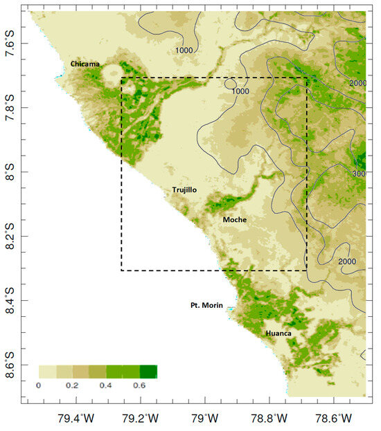
Figure A1.
Moche coastal area satellite vegetation color fraction, same as Figure 5A but zoomed to show irrigated river valleys; smoothed topographic contours > 1000 m overlain; dashed box is the area for extraction of time series.
Figure A1.
Moche coastal area satellite vegetation color fraction, same as Figure 5A but zoomed to show irrigated river valleys; smoothed topographic contours > 1000 m overlain; dashed box is the area for extraction of time series.
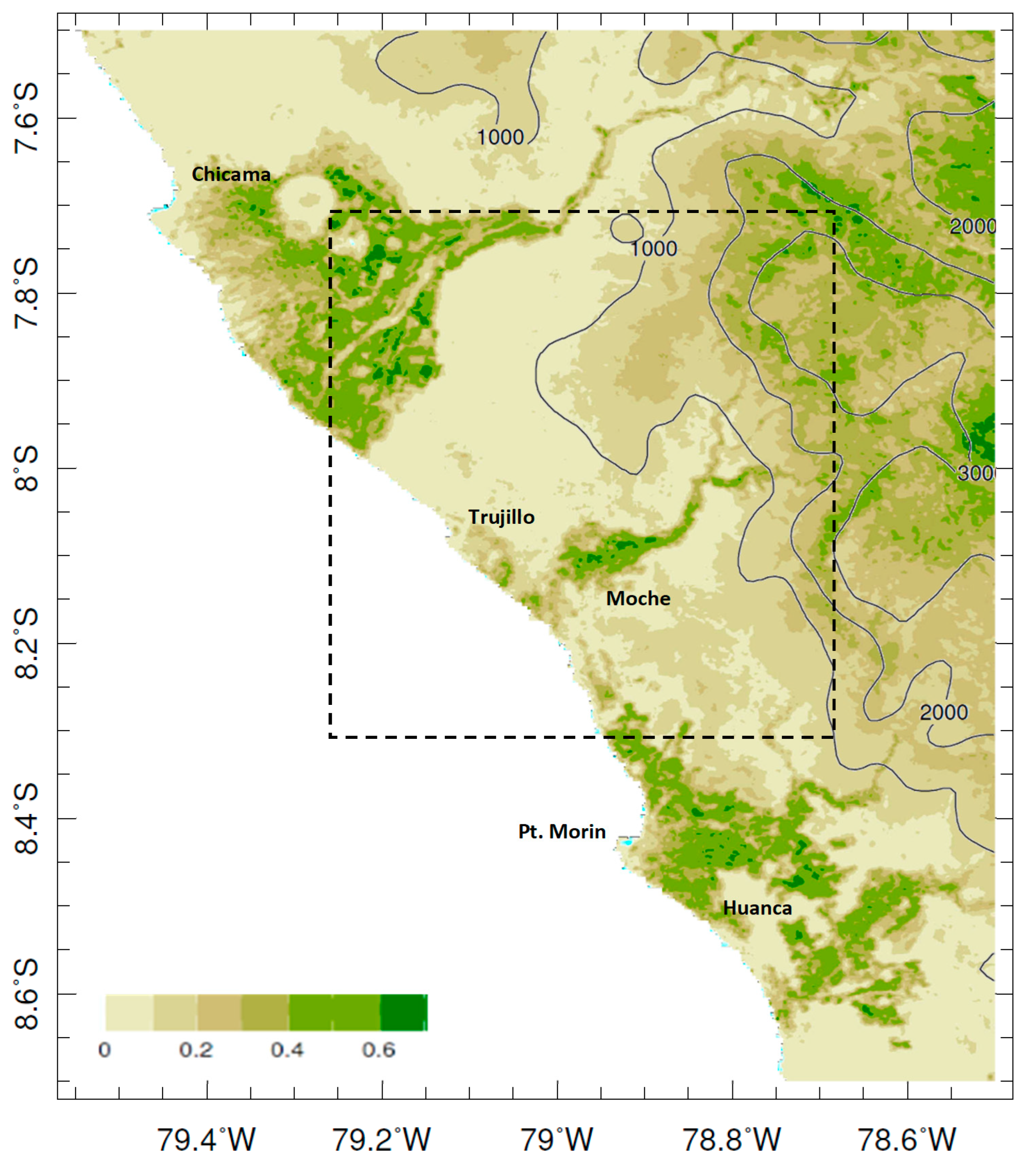
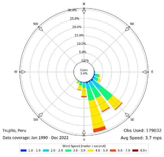
Figure A2.
Trujillo airport wind rose, illustrating the prevalence of airflow from SSE.
Figure A2.
Trujillo airport wind rose, illustrating the prevalence of airflow from SSE.

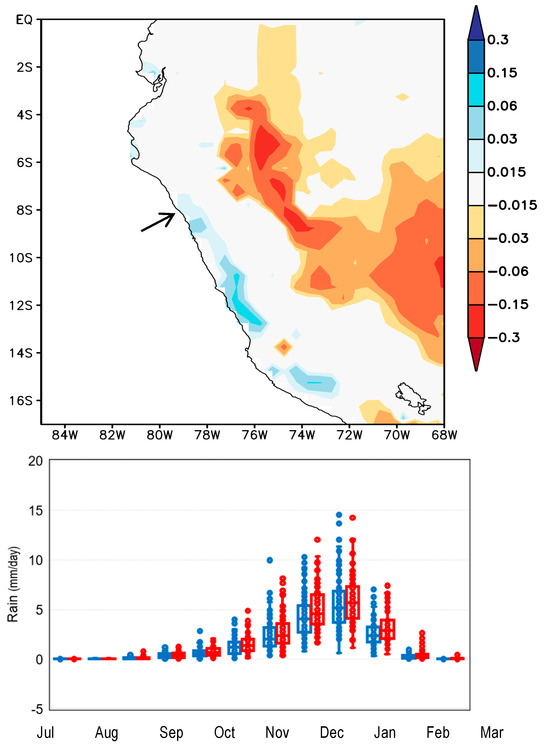
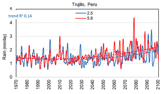
Figure A3.
(upper) HAD-coupled ensemble model soil moisture trend 1970–2070 (mm/yr) with 5.8 W/m2 scenario; arrow points to Trujillo. Projection of Moche area precipitation under 2.5 (blue) and 5.8 W/m2 (red) scenarios, based on CNRM- and MRI-coupled ensemble models: box-whisker of annual cycle (middle) and smoothed time series (lower) with 2nd-order trend and R2 fit.
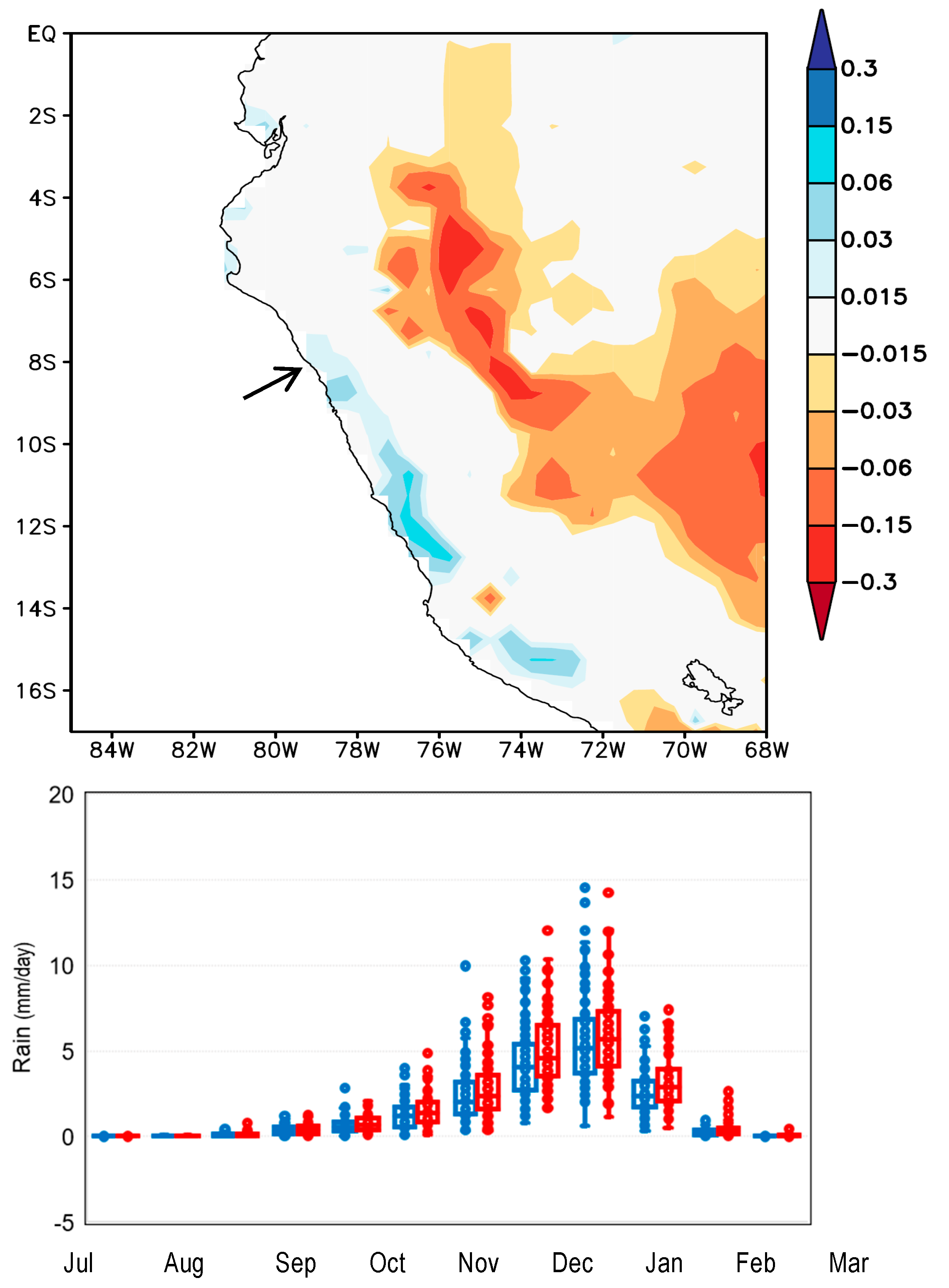
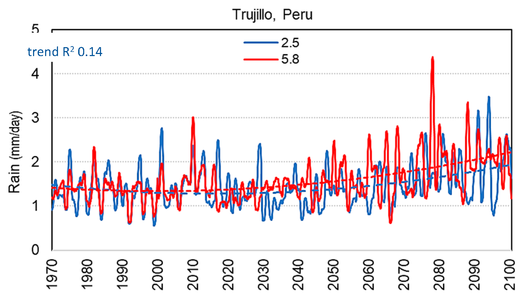
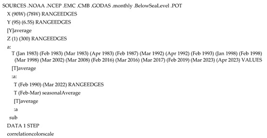
Figure A4.
IRI climate website subroutine to calculate the cross-shelf sea temperature anomalies for composite wet months on the north coast of Peru, resulting in Figure 8C (right).
Figure A4.
IRI climate website subroutine to calculate the cross-shelf sea temperature anomalies for composite wet months on the north coast of Peru, resulting in Figure 8C (right).
References
- Penven, P.; Echevin, V.; Pasapera, J.; Colas, F.; Tam, J. Average circulation, seasonal cycle, and mesoscale dynamics of the Peru Current System: A modeling approach. J. Geophys. Res. Ocean. 2005, 110, 10021. [Google Scholar] [CrossRef]
- Chamorro-Gomez, A.; Colas, F.; Echevin, V.; Tam, J. Characterization of coastal jets over the Peruvian sea using the WRF regional model. Bol. Inst. Mar. Peru 2022, 37, 271–284. [Google Scholar]
- Briceño-Zuluaga, F.; Flores-Aqueveque, V.; Nogueira, J.; Castillo, A.; Cardich, J.; Rutllant, J.; Caquineau, S.; Sifeddine, A.; Salvatteci, R.; Valdes, J.; et al. Surface wind strength and sea surface temperature connections along the south peruvian coast during the last 150 years. Aeolian Res. 2023, 61, 100855. [Google Scholar] [CrossRef]
- Dewitte, B.; Vazquez-Cuervo, J.; Goubanova, K.; Illig, S.; Takahashi, K.; Cambon, G.; Purca, S.; Correa, D.; Gutierrez, D.; Sifeddine, A.; et al. Change in El Niño flavours over 1958–2008: Implications for the long-term trend of the upwelling off Peru. Deep. Sea Res. Part II Top. Stud. Oceanogr. 2012, 77, 143–156. [Google Scholar] [CrossRef]
- Quispe-Ccalluari, C.; Tam, J.; Demarcq, H.; Chamorro, A.; Espinoza-Morriberón, D.; Romero, C.; Dominguez, N.; Ramos, J.; Oliveros-Ramos, R. An index of coastal thermal effects of El Niño Southern Oscillation on the Peruvian Upwelling Ecosystem. Int. J. Clim. 2018, 38, 3191–3201. [Google Scholar] [CrossRef]
- Philander, S.G. El Niño, La Niña, and the Southern Oscillation; Academic Press: Cambridge, UK, 1990; p. 293. [Google Scholar]
- Lenters, J.D.; Cook, K.H. Summertime precipitation variability over South America: Role of the large-scale circulation. Mon. Weather. Rev. 1999, 127, 409–431. [Google Scholar] [CrossRef]
- Kao, H.; Yu, J. Contrasting eastern- and central-Pacific types of ENSO. J. Clim. 2009, 22, 615–632. [Google Scholar] [CrossRef]
- Hu, X.; Yang, S.; Cai, M. Contrasting the eastern- and central- Pacific El Niño: Process-based feedback attribution. Clim. Dyn. 2016, 47, 2413–2424. [Google Scholar] [CrossRef]
- Alizadeh-Choobari, O. Contrasting global teleconnection features of the eastern Pacific and central Pacific El Niño events. Dyn. Atmos. Ocean. 2017, 80, 139–154. [Google Scholar] [CrossRef]
- Mantua, N.J.; Hare, S.R. The Pacific Decadal Oscillation. J. Oceanogr. 2002, 59, 35–44. [Google Scholar] [CrossRef]
- Cai, W.; McPhaden, M.J.; Grimm, A.M.; Rodrigues, R.R.; Taschetto, A.S.; Garreaud, R.D.; Dewitte, B.; Poveda, G.; Ham, Y.-G.; Santoso, A.; et al. Climate impacts of the El Niño–Southern Oscillation on South America, Nature Rev. Earth Environ. 2020, 1, 215–231. [Google Scholar]
- Sulca, J.; Takahashi, K.; Espinoza, J.-C.; Vuille, M.; Lavado-Casimiro, W. Impacts of different ENSO flavors and tropical Pacific convection variability (ITCZ, SPCZ) on austral summer rainfall in South America, with a focus on Peru. Int. J. Clim. 2018, 38, 420–435. [Google Scholar] [CrossRef]
- Gonzales, E.; Ingol, E. Determination of a new coastal ENSO oceanic index for northern Peru. Climate 2021, 9, 71. [Google Scholar] [CrossRef]
- Caramanica, A.; Mesia, L.H.; Morales, C.R.; Huckleberry, G.; Castillo, B.L.J.; Quilter, J. El Niño resilience farming on the north coast of Peru. Proc. Nat. Acad. Sci. USA 2020, 117, 24127–24137. [Google Scholar] [CrossRef] [PubMed]
- White, W.B. Tropical coupled Rossby waves in the Pacific ocean–atmosphere system. J. Phys. Oceanogr. 2020, 30, 1245–1264. [Google Scholar] [CrossRef]
- Rydbeck, A.V.; Jensen, T.G.; Flatau, M. Characterization of intra-seasonal Kelvin waves in the equatorial Pacific Ocean. J. Geophys. Res. Ocean. 2019, 124, 2028–2053. [Google Scholar] [CrossRef]
- Bourrel, L.; Rau, P.; Dewitte, B.; Labat, D.; Lavado, W.; Coutaud, A.; Vera, A.; Alvarado, A.; Ordoñez, J. Low-frequency modulation and trend of the relationship between ENSO and precipitation along the northern to centre Peruvian Pacific coast. Hydrol. Process. 2015, 29, 1252–1266. [Google Scholar] [CrossRef]
- Sanabria, J.; Bourrel, L.; Dewitte, B.; Frappart, F.; Rau, P.; Solis, O.; Labat, D. Rainfall along the coast of Peru during strong El Niño events. Intl. J. Climatol. 2018, 38, 1737–1747. [Google Scholar] [CrossRef]
- Douglas, M.W.; Mejia, J.; Ordinola, N.; Boustead, J. Synoptic variability of rainfall and cloudiness along the coast of northern Peru and Ecuador during the 1997/98 El Niño Event. Mon. Wea. Rev. 2009, 137, 116–136. [Google Scholar] [CrossRef]
- Rodríguez-Morata, C.; Díaz, H.F.; Ballesteros-Canovas, J.A.; Rohrer, M.; Stoffel, M. The anomalous 2017 coastal El Niño event in Peru. Clim. Dyn. 2019, 52, 5605–5622. [Google Scholar] [CrossRef]
- Recalde-Coronel, G.C.; Zaitchik, B.; Pan, W.K. Madden–Julian oscillation influence on sub-seasonal rainfall variability on the west of South America. Clim. Dyn. 2020, 54, 2167–2185. [Google Scholar] [CrossRef] [PubMed]
- Rosales, A.G.; Junquas, C.; da Rocha, R.P.; Condom, T.; Espinoza, J.-C. Valley–mountain circulation associated with the diurnal cycle of precipitation in the tropical andes (Santa River Basin, Peru). Atmosphere 2022, 13, 344. [Google Scholar] [CrossRef]
- Maes, W.H.; Gentine, P.; Verhoest, N.E.C.; Miralles, D.G. Potential evaporation at eddy-covariance sites across the globe. Hydrol. Earth Syst. Sci. 2018, 23, 925–948. [Google Scholar] [CrossRef]
- McMahon, T.A.; Peel, M.C.; Lowe, L.; Srikanthan, R.; McVicar, T.R. Estimating actual, potential, reference crop and pan evaporation using standard meteorological data: A pragmatic synthesis. Hydrol. Earth Syst. Sci. 2013, 17, 1331–1363. [Google Scholar] [CrossRef]
- Saha, S.; Moorthi, S.; Wu, X.; Wang, J.; Nadiga, S.; Tripp, P.; Behringer, D.; Hou, Y.-T.; Chuang, H.-Y.; Iredell, M.; et al. The NCEP climate forecast system version 2. J. Clim. 2014, 27, 2185–2208. [Google Scholar] [CrossRef]
- Johnson, S.J.; Stockdale, T.N.; Ferranti, L.; Balmaseda, M.A.; Molteni, F.; Magnusson, L.; Tietsche, S.; Decremer, D.; Weisheimer, A.; Balsamo, G.; et al. SEAS5: The new ECMWF seasonal forecast system. Geosci. Model Dev. 2019, 12, 1087–1117. [Google Scholar] [CrossRef]
- Harrigan, S.; Zsoter, E.; Alfieri, L.; Prudhomme, C.; Salamon, P.; Wetterhall, F.; Barnard, C.; Cloke, H.; Pappenberger, F. GloFAS-ERA5 operational global river discharge reanalysis 1979–present, Earth Syst. Sci. Data 2020, 12, 2043–2060. [Google Scholar]
- Faugère, Y.; Taburet, G.; Ballarotta, M.; Pujol, I.; Legeais, J.F.; Maillard, G.; Chloe, D.; Quentin, D.; Marine, L.; Antonio, S.R.; et al. DUACS-dt21: 28 years of reprocessed sea level altimetry products. In Proceedings of the Assembly Proceedings EGU22-7479, Vienna, Austria, 23–27 May 2022. [Google Scholar]
- Hersbach, H.; Bell, B.; Berrisford, P.; Hirahara, S.; Horányi, A.; Muñoz-Sabater, J.; Nicolas, J.; Peubey, C.; Radu, R.; Schepers, D.; et al. The ERA5 global reanalysis. Qtr. J. R. Meteo. Soc. 2020, 146, 1999–2049. [Google Scholar] [CrossRef]
- Behringer, D.W. The global ocean data assimilation system (GODAS) at NCEP. In Proceedings of the 11th Symposium on Integrated Observing and Assimilation Systems for the Atmosphere, Oceans, and Land Surface, San Antonio, TX, USA, 14–18 January 2007. [Google Scholar]
- Hou, A.Y.; Kakar, R.K.; Neeck, S.; Azarbarzin, A.A.; Kummerow, C.D.; Kojima, M.; Oki, R.; Nakamura, K.; Iguchi, T. The Global Precipitation Measurement mission. Bull. Am. Meteorol. Soc. 2014, 95, 701–722. [Google Scholar] [CrossRef]
- Ghiggi, G.; Humphrey, V.; Seneviratne, S.I.; Gudmundsson, L. G-RUN ENSEMBLE: A multi-forcing observation-based global runoff reanalysis. Water Resour. Res. 2021, 57, e2020WR028787. [Google Scholar] [CrossRef]
- Rayner, N.A.; Parker, D.E.; Horton, E.B.; Horton, E.B.; Folland, C.K.; Alexander, L.V.; Rowell, D.P.; Kent, E.C.; Kaplan, A. Global analyses of sea surface temperature, sea ice, and night marine air temperature since the late nineteenth century. J. Geophys. Res. 2003, 108, 4407. [Google Scholar] [CrossRef]
- Gelaro, R.; McCarty, W.; Suárez, M.J.; Todling, R.; Molod, A.; Takacs, L.; Randles, C.A.; Darmenov, A.; Bosilovich, M.G.; Reichle, R.; et al. The modern-era retrospective analysis for research and applications, v2 (MERRA2). J. Clim. 2017, 30, 5419–5454. [Google Scholar] [CrossRef] [PubMed]
- Pinzon, J.E.; Tucker, C.J. A non-stationary AVHRR NDVI time series. Remote Sens. 2014, 6, 6929–6960. [Google Scholar] [CrossRef]
- Zhang, T.; Hoell, A.; Perlwitz, J.; Eischeid, J.; Murray, D.; Hoerling, M.; Hamill, T.M. Towards probabilistic multi-variate ENSO monitoring. Geophys. Res. Lett. 2019, 46, 10532–10540. [Google Scholar] [CrossRef]
- Lee, H.-T.; Gruber, A.; Ellingson, R.G.; Laszlo, I. Development of the HIRS outgoing longwave radiation climate dataset. J. Atmos. Ocean. Technol. 2007, 24, 2029–2047. [Google Scholar] [CrossRef]
- Echevin, V.; Colas, F.; Espinoza-Morriberon, D.; Vasquez, L.; Anculle, T.; Gutierrez, D. Forcing and evolution of the 2017 coastal El Niño off northern Peru and Ecuador, Frontiers Mar. Science 2018, 5, 3389. [Google Scholar]
- Grados, C.; Chaigneau, A.; Echevin, V.; Dominguez, N. Upper ocean hydrology of the northern Humboldt Current system at seasonal, interannual and interdecadal scales. Prog. Oceanogr. 2018, 165, 123–144. [Google Scholar] [CrossRef]
- Roundy, P.E.; Kiladis, G.N. Observed relationships between oceanic kelvin waves and atmospheric forcing. J. Clim. 2006, 19, 5253–5272. [Google Scholar] [CrossRef]
- Jury, M.R. Global wave-2 structure of ENSO-modulated convection. Int. J. Clim. 2019, 39, 2438–2448. [Google Scholar] [CrossRef]
- Wei, Y.; Ren, H.-L. Modulation of ENSO on fast and slow MJO modes during boreal winter. J. Clim. 2019, 32, 7483–7506. [Google Scholar] [CrossRef]
- French, A.; Mechler, R.; Arestegui, M.; MacClune, K.; Cisneros, A. Root causes of recurrent catastrophe: The political ecology of El Nino-related disasters in Peru. Int. J. Disaster Risk Reduct. 2020, 47, 101539. [Google Scholar] [CrossRef]


Disclaimer/Publisher’s Note: The statements, opinions and data contained in all publications are solely those of the individual author(s) and contributor(s) and not of MDPI and/or the editor(s). MDPI and/or the editor(s) disclaim responsibility for any injury to people or property resulting from any ideas, methods, instructions or products referred to in the content. |
© 2024 by the authors. Licensee MDPI, Basel, Switzerland. This article is an open access article distributed under the terms and conditions of the Creative Commons Attribution (CC BY) license (https://creativecommons.org/licenses/by/4.0/).