Introducing a Parallel Genetic Algorithm for Global Optimization Problems

Abstract

The topic of efficiently finding the global minimum of multidimensional functions is widely applicable to numerous problems in the modern world. Many algorithms have been proposed to address these problems, among which genetic algorithms and their variants are particularly notable. Their popularity is due to their exceptional performance in solving optimization problems and their adaptability to various types of problems. However, genetic algorithms require significant computational resources and time, prompting the need for parallel techniques. Moving in this research direction, a new global optimization method is presented here that exploits the use of parallel computing techniques in genetic algorithms. This innovative method employs autonomous parallel computing units that periodically share the optimal solutions they discover. Increasing the number of computational threads, coupled with solution exchange techniques, can significantly reduce the number of calls to the objective function, thus saving computational power. Also, a stopping rule is proposed that takes advantage of the parallel computational environment. The proposed method was tested on a broad array of benchmark functions from the relevant literature and compared with other global optimization techniques regarding its efficiency.

1. Introduction

Typically, the task of locating the global minimum [1] of a function $f:S\to R,S\subset R^n$ is defined as follows:

$$x^{*}=\arg \underset{x\in S}{min}f\left(x\right).$$

(1)

where the set (S) is as follows:

$$S=\left[a_1,b_1\right]\otimes \left[a_2,b_2\right]\otimes \dots \left[a_n,b_n\right]$$

The values $a_i$ and $b_i$ are the left and right bounds, respectively, for the point $x_i$. A systematic review of the optimization procedure can be found in the work of Fouskakis [2].

The previously defined problem has been tackled using a variety of methods, which have been successfully applied to a wide range of problems in various fields, such as medicine [3,4], chemistry [5,6], physics [7,8,9], economics [10,11], etc. Global optimization methods are divided into two main categories: deterministic and stochastic methods [12]. The first category belongs to the interval methods [13,14], where the set (S) is iteratively divided into subregions, and those that do not contain the global solution are discarded based on predefined criteria. Many related works have been published in the area of deterministic methods, including the work of Maranas and Floudas, who proposed a deterministic method for chemical problems [15], the TRUST method [16], the method suggested by Evtushenko and Posypkin [17], etc. In the second category, the search for the global minimum is based on randomness. Also, stochastic optimization methods are commonly used because they can be programmed more easily and do not depend on any previous information about the objective problem. Some stochastic optimization methods that have been used by researchers include ant colony optimization [18,19], controlled random search [20,21,22], particle swarm optimization [23,24,25], simulated annealing [26,27,28], differential evolution [29,30], and genetic algorithms [31,32,33]. Finally, there is a plethora of research referring to metaheuristic algorithms [34,35,36], offering new perspectives and solutions to problems in various fields.

The current work proposes a series of modifications in order to effectively parallelize the widely adopted method of genetic algorithms for solving Equation (1). Genetic algorithms, initially proposed by John Holland, constitute a fundamental technique in the field of stochastic methods [37]. Inspired by biology, these algorithms simulate the principles of evolution, including genetic mutation, natural selection, and the exchange of genetic material [38]. The integration of genetic algorithms with machine learning has proven effective in addressing complex problems and validating models. This interaction is highlighted in applications such as the design and optimization of 5G networks, contributing to path loss estimation and improving performance in indoor environments [39]. It is also applied to optimizing the movement of digital robots [40] and conserving energy in industrial robots with two arms [41]. Additionally, genetic algorithms have been employed to find optimal operating conditions for motors [42], optimize the placement of electric vehicle charging stations [43], manage energy [44], and have applications in other fields such as medicine [45,46] and agriculture [47].

Although genetic algorithms have proven to be effective, the optimization process requires significant computational resources and time. This emphasizes the necessity of implementing parallel techniques, as the execution of algorithms is significantly accelerated by the combined use of multiple computational resources. Modern parallel programming techniques include the message-passing interface (MPI) [48] and the OpenMP library [49]. Parallel programming techniques have also been incorporated in various cases into global optimization, such as the combination of simulated annealing and parallel techniques [50], the use of parallel methods in particle swarm optimization [51], the incorporation of radial basis functions in parallel stochastic optimization [52], etc. One of the main advantages of genetic algorithms over other global optimization techniques is that they can be easily parallelized and exploit modern computing units as well as the previously mentioned parallel programming techniques.

In the relevant literature, two major categories of parallel genetic algorithms appear, namely, island genetic algorithms and cellular genetic algorithms [53]. The island model is a parallel genetic algorithm (PGA), which manages several subpopulations on separate islands, and executes the genetic algorithm process on each island simultaneously for a different set of solutions. Island models have been utilized in various cases, such as molecular sequence alignment [54], the quadratic assignment problem [55], the placement of sensors/actuators in large structures [56], etc. Also, recently, Tsoulos et al. proposed an implementation of an island PGA [57]. Regarding the parallel cellular model of genetic algorithms, solutions are organized into a grid. Various diverse operators, such as crossovers and mutations, are applied to neighboring regions within the grid. For each solution, a descendant factor is created, replacing its position within the birth region. The model is flexible regarding the structure of the grid, neighborhood strategies, and settings. Implementations may involve multiple processors or graphical processing units, with information exchange possible through physical communication networks. The theory of parallel genetic algorithms has been thoroughly presented by a number of researchers in the literature [58,59]. Also, parallel genetic algorithms have been incorporated in combinatorial optimization [60].

The proposed method is based on the island technique and suggests a number of improvements to the general scheme of parallel Genetic Algorithms. Among these improvements are a series of techniques for propagating optimal solutions among islands that aim to speed up the convergence of the overall algorithm. In addition, the individual islands of the genetic algorithm periodically apply a local minimization technique with two goals: to discover the most accurate local minima of the objective function and to speed up the convergence of the overall algorithm without wasting computing power on previously discovered function values. Furthermore, an efficient termination rule based on asymptotic considerations, which was validated across a series of global optimization methods, is also incorporated into the current algorithm. The proposed method was applied to a series of problems appearing in the relevant literature. The experimental results indicate that the new method can effectively find the global minimum of the functions in a large percentage of cases, and the above modifications significantly accelerated the discovery of the global minimum as the number of individual islands in the genetic algorithm increased.

The remainder of the article follows this structure: In Section 2, the genetic algorithm is analyzed, and the parallelization, dissemination techniques (PT or migration methodologies), and termination criteria are discussed. Subsequently, in Section 3, the test functions used are presented in detail, along with the experimental results. Finally, in Section 4, some conclusions are outlined, and future explorations are formulated.

2. Method Description

This section begins with a detailed description of the base genetic algorithm and continues providing the details of the suggested modifications.

2.1. The Genetic Algorithm

Genetic algorithms are inspired by natural selection and the process of evolution. In their basic form, they start with an initial population of chromosomes, representing possible solutions to a specific problem. Each chromosome is represented as a “gene”, and its length is equal to the dimension of the problem. The algorithm processes these solutions through iterative steps, replicating and evolving the population of solutions. In each generation, the selected solutions are crossed and mutated to improve their fit to the problem. As generations progress, the population converges toward solutions with improved fit to the problem. Important factors affecting genetic algorithm performance include population size, selection rate, crossover and mutation probabilities, and strategic replacement of solutions. The choice of these parameters affects the ability of the algorithm to explore the solution space and converge to the optimal result. Subsequently, the operation of the genetic algorithm is presented through the replication and advancement of solution populations, step by step [61,62]. The steps of a typical genetic algorithm is shown in Algorithm 1.

2.2. Parallelization of Genetic Algorithm and Propagation Techniques

In the parallel island model of Figure 1, an evolving population is divided into various “islands”, each working concurrently to optimize a specific set of solutions. In this figure, each island implements a separate genetic algorithm as described in Section 2.1. The steps of the overall algorithm are also presented through a series of steps in Algorithm 2. In contrast to classical parallelization, which handles a central population, the island model features decentralized populations evolving independently. Each island exchanges information with others at specific points in evolution through migration, where solutions move from one island to another, influencing the overall convergence toward the optimal solution. Migration settings determine how often they occur and which solutions are selected for exchange. Each island can follow a similar search strategy, but for more variety or faster convergence, different approaches can be employed. Islands may have identical or diverse strategies, providing flexibility and efficiency in exploring the solution space. To implement this parallel model, each island is connected to a computational resource. For instance, as depicted in images of Figure 2, the execution of the parallel island model involves five islands, each managing a distinct set of solutions using five processor units (PUs). During the migration process, information related to solutions is exchanged among PUs. Figure 2 also depicts the four different techniques for spreading the chromosomes with the best functional values. In Figure 2a, we observe the migration of the best chromosomes from one island to another (randomly chosen). In Figure 2b, migration occurs from a randomly chosen island to all others. In Figure 2c, it occurs from all islands to a randomly chosen one, and finally, in Figure 2d, migration occurs from each island to all others.

Algorithm 1 The steps of the genetic algorithm.

Initialization step. (a) Set $N_c$ as the number of chromosomes. (b) Set $N_g$ the maximum number of allowed generations. (c) Initialize randomly $N_c$ chromosomes in S. Each chromosome denotes a potential solution to the problem of Equation (1). (d) Set as $p_s$ the selection rate of the algorithm, with $p_s\le 1$. (e) Set as $p_m$ the mutation rate, with $p_m\le 1$. (f) Set k = 0 as the generation counter. Fitness calculation step. (a) For every chromosome $g_i,i=1,\dots ,N_c$ Calculate the fitness $f_i=f\left(g_i\right)$ of chromosome $g_i$. Selection step. The chromosomes are sorted with respect to their fitness values. Denote as $N_b$ the integer part of $\left(1-p_s\right)\times N_c$ chromosomes with the lowest fitness values. These chromosomes will be copied to the next generation. The rest of the chromosomes will be replaced by offspring created in the crossover procedure. Each offspring is created from two chromosomes (parents) of the population through the tournament selection process. The procedure for tournament selection is as follows: A set of $N_t>1$ randomly selected chromosomes is formed, and the individual with the lowest fitness value from this set is selected as a parent. Crossover step. Two selected solutions (parents) are combined to create new solutions (offspring). During crossover, genes are exchanged between parents, introducing diversity. For each selected pair of parents $(z,w)$, two additional chromosomes, represented by $\tilde{z}$ and $\tilde{w}$, are generated through the following equations. $$\begin{array}{ccc}\hfill \widetilde{z_i}& =& a_i{z}_i+\left(1-a_i\right)w_i\hfill \\ \hfill \widetilde{w_i}& =& a_i{w}_i+\left(1-a_i\right)z_i\hfill \end{array}$$ (2) where $i=1,\dots ,n$. The values $a_i$ are uniformly distributed random numbers, with $a_i\in [-0.5,1.5]$ [63]. Replacement step. (a) For $i=N_b+1$ to $N_c$ do Replace $g_i$ using the next offspring created in the crossover procedure. (b) End For Mutation step. Some genes in the offspring are randomly modified. This introduces more diversity into the population and helps identify new solutions. (a) For every chromosome $g_i,i=1,\dots ,N_c$: For each element $j=1,\dots ,n$ of $g_i$, a uniformly distributed random number $r\in \left[0,1\right]$ is drawn. The element is altered randomly if $r\le p_m$. (b) End For Set $k=k+1$. If the termination criterion defined in the work of Tsoulos [64], which is outlined in Section 2.3, is met, or $k>N_g$, then go to the local search step; otherwise, go to step 2a. Local search step. To improve the success in finding better solutions, a process of local optimization search is implemented. In the present study, the Broyden–Fletcher–Goldfarb–Shanno (BFGS) variant proposed by Powell [65] is employed as the local search procedure. This procedure is applied to the chromosome in the population with the lowest fitness value.

Algorithm 2 The overall algorithm.

Set $N_I$ as the total number of parallel processing units. Set $N_R$ as the number of generations, after which, each processing unit will send its best chromosomes to the remaining processing units. Set $N_P$ as the number of migrated chromosomes between the parallel processing units. Set $PT$ as the propagation technique. Set $k=0$ as the generation number. For $j=1,\dots ,N_I$, perform in parallel (a) Execute a generation of the GA algorithm described in Algorithm 1 on processing unit j. (b) If $K\mathbf{mod}{N}_R=0,$ then Obtain the best $N_P$ chromosomes from algorithm j. Propagate these $N_P$ chromosomes to the rest of the processing units using a propagation scheme that will be subsequently described. (c) End If End For Update $k=k+1$ Check the proposed termination rule. If the termination rule is valid, then go to step 9a; otherwise, go to step 6. (a) Terminate and report the best value from all processing units. Apply a local search procedure to this located value to enhance the located global minimum.

The migration or propagation techniques, as described in this study, are periodically and synchronously performed in $N_R$ iterations on each processing unit. Below are the migration techniques that could be defined:

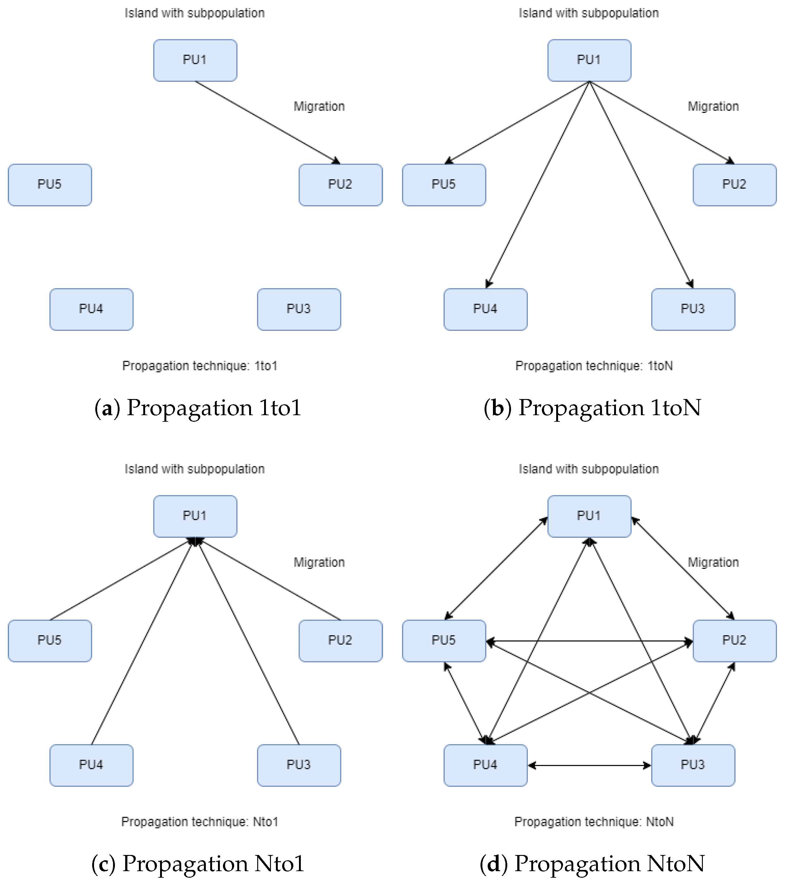
• 1to1: Optimal solutions migrate from a random island to another random one, replacing the worst solutions (see Figure 2a).
• 1toN: Optimal solutions migrate from a random island to all others, replacing the worst solutions (see Figure 2b).
• Nto1: All islands send their optimal solutions to a random island, replacing the worst solutions (see Figure 2c).
• NtoN: All islands send their optimal solutions to all other islands, replacing the worst solutions (see Figure 2d).

If we assume that the migration method “1toN” is executed, then a random island will transfer chromosomes to the other islands, except for itself. However, we keep the label “N” instead of “N-1” because the chromosomes exist on the island that sends them. The number of solutions participating in the migration and replacement process is fully customizable and will be discussed in the experiments below.

2.3. Termination Rule

The termination criterion employed in this study was originally introduced in the research conducted by Tsoulos [64] and it is formulated as follows:

• In each generation k, the chromosome $g^{*}$ with the best functional value $f\left(g^{*}\right)$ is retrieved from the population. If this value does not change for a number of generations, then the algorithm should probably terminate.
• Consider ${\sigma }^{\left(k\right)}$ as the associated variance of the quantity $f\left(g^{*}\right)$ at generation k. The algorithm terminates when

  $$k\ge N_g\mathrm{or}{\sigma }^{\left(k\right)}\le \frac{{\sigma }^{\left(k_{\mathrm{last}}\right)}}{2}$$

  where $k_{\mathrm{last}}$ is the last generation where a lower value of $f\left(g^{*}\right)$ is discovered.

3. Experiments

A series of benchmark functions from the relevant literature is introduced here, along with the conducted experiments and a discussion of the experimental results.

3.1. Test Functions

To assess the effectiveness of the proposed method in locating the overall minimum of functions, a set of well-known test functions cited in the relevant literature [66,67] was employed. The functions used here are as follows:

• The Bent cigar function is defined as follows:

  $$f\left(x\right)=x_1^2+{10}^6\sum _{i=2}^n{x}_i^2$$

  with the global minimum $f\left(x^{*}\right)=0$. For the conducted experiments, the value $n=10$ was used.
• The Bf1 function (Bohachevsky 1) is defined as follows:

  $$f\left(x\right)=x_1^2+2x_2^2-\frac{3}{10}cos\left(3\pi x_1\right)-\frac{4}{10}cos\left(4\pi x_2\right)+\frac{7}{10}$$

  with $x\in {[-100,100]}^2$.

• The Bf2 function (Bohachevsky 2) is defined as follows:

  $$f\left(x\right)=x_1^2+2x_2^2-\frac{3}{10}cos\left(3\pi x_1\right)cos\left(4\pi x_2\right)+\frac{3}{10}$$

  with $x\in {[-50,50]}^2$.
• The Branin function is given by $f\left(x\right)={\left(x_2-\frac{5.1}{4{\pi }^2}{x}_1^2+\frac{5}{\pi }{x}_1-6\right)}^2+10\left(1-\frac{1}{8\pi }\right)cos\left(x_1\right)+10$ with $-5\le x_1\le 10,0\le x_2\le 15$ and with $x\in {[-10,10]}^2$.
• The CM function. The cosine mixture function is given by the following:

  $$f\left(x\right)=\sum _{i=1}^n{x}_i^2-\frac{1}{10}\sum _{i=1}^{n}cos\left(5\pi x_i\right)$$

  with $x\in {[-1,1]}^n$. The value $n=4$ was used in the conducted experiments.
• Discus function. The function is defined as follows:

  $$f\left(x\right)={10}^6{x}_1^2+\sum _{i=2}^n{x}_i^2$$

  with global minimum $f\left(x^{*}\right)=0.$ For the conducted experiments, the value $n=10$ was used.
• The Easom function. The function is given by the following equation:

  $$f\left(x\right)=-cos\left(x_1\right)cos\left(x_2\right)exp\left({\left(x_2-\pi \right)}^2-{\left(x_1-\pi \right)}^2\right)$$

  with $x\in {[-100,100]}^2$.
• The exponential function. The function is given by the following:

  $$f\left(x\right)=-exp\left(-0.5\sum _{i=1}^n{x}_i^2\right),-1\le x_i\le 1$$
  The global minimum is situated at $x^{*}=(0,0,\dots ,0)$, with a value of $-1$. In our experiments, we applied this function for $n=4,16,64$, and referred to the respective instances as EXP4, EXP16, EXP64, and EXP100.
• Griewank2 function. The function is given by the following:

  $$f\left(x\right)=1+\frac{1}{200}\sum _{i=1}^2{x}_i^2-\prod _{i=1}^2\frac{cos\left(x_i\right)}{\sqrt{\left(i\right)}},x\in {[-100,100]}^2$$

The global minimum is located at the $x^{*}=(0,0,\dots ,0)$ with a value of 0.

• Gkls function. $f\left(x\right)=Gkls(x,n,w)$ is a function with w local minima, described in [68] with $x\in {[-1,1]}^n$, and n is a positive integer between 2 and 100. The value of the global minimum is −1, and in our experiments, we used $n=2,3$ and $w=50,100$.
• Hansen function. $f\left(x\right)={\sum }_{i=1}^{5}icos\left[(i-1)x_1+i\right]{\sum }_{j=1}^{5}jcos\left[(j+1)x_2+j\right]$, $x\in {[-10,10]}^2$. The global minimum of the function is −176.541793.
• Hartman 3 function. The function is given by the following:

  $$f\left(x\right)=-\sum _{i=1}^4{c}_{i}exp\left(-\sum _{j=1}^3{a}_{ij}{\left(x_j-p_{ij}\right)}^2\right)$$

  with $x\in {[0,1]}^3$ and $a=\left(\begin{array}{ccc}3& 10& 30\\ 0.1& 10& 35\\ 3& 10& 30\\ 0.1& 10& 35\end{array}\right),c=\left(\begin{array}{c}1\\ 1.2\\ 3\\ 3.2\end{array}\right)$ and

  $$p=\left(\begin{array}{ccc}0.3689& 0.117& 0.2673\\ 0.4699& 0.4387& 0.747\\ 0.1091& 0.8732& 0.5547\\ 0.03815& 0.5743& 0.8828\end{array}\right)$$
  The value of the global minimum is −3.862782.
• Hartman 6 function.

  $$f\left(x\right)=-\sum _{i=1}^4{c}_{i}exp\left(-\sum _{j=1}^6{a}_{ij}{\left(x_j-p_{ij}\right)}^2\right)$$

  with $x\in {[0,1]}^6$ and $a=\left(\begin{array}{cccccc}10& 3& 17& 3.5& 1.7& 8\\ 0.05& 10& 17& 0.1& 8& 14\\ 3& 3.5& 1.7& 10& 17& 8\\ 17& 8& 0.05& 10& 0.1& 14\end{array}\right),c=\left(\begin{array}{c}1\\ 1.2\\ 3\\ 3.2\end{array}\right)$ and

  $$p=\left(\begin{array}{cccccc}0.1312& 0.1696& 0.5569& 0.0124& 0.8283& 0.5886\\ 0.2329& 0.4135& 0.8307& 0.3736& 0.1004& 0.9991\\ 0.2348& 0.1451& 0.3522& 0.2883& 0.3047& 0.6650\\ 0.4047& 0.8828& 0.8732& 0.5743& 0.1091& 0.0381\end{array}\right)$$

  the value of the global minimum is −3.322368.
• The high-conditioned elliptic function is defined as follows:

  $$f\left(x\right)=\sum _{i=1}^n{\left({10}^6\right)}^{\frac{i-1}{n-1}}{x}_i^2$$
  Featuring a global minimum at $f\left(x^{*}\right)=0$, the experiments were conducted using the value $n=10$.
• Potential function. As a test case, the molecular conformation corresponding to the global minimum of the energy of N atoms interacting via the Lennard–Jones potential [69] is utilized. The function to be minimized is defined as follows:

  $$V_{LJ}\left(r\right)=4ϵ\left[{\left(\frac{\sigma }{r}\right)}^{12}-{\left(\frac{\sigma }{r}\right)}^6\right]$$

  (3)
  In the current experiments, two different cases were studied: $N=3,5$.
• Rastrigin function. This function is given by the following:

  $$f\left(x\right)=x_1^2+x_2^2-cos\left(18x_1\right)-cos\left(18x_2\right),x\in {[-1,1]}^2$$
• Shekel 7 function.

  $$f\left(x\right)=-\sum _{i=1}^7\frac{1}{(x-a_i){(x-a_i)}^T+c_i}$$

  with $x\in {[0,10]}^4$ and $a=\left(\begin{array}{cccc}4& 4& 4& 4\\ 1& 1& 1& 1\\ 8& 8& 8& 8\\ 6& 6& 6& 6\\ 3& 7& 3& 7\\ 2& 9& 2& 9\\ 5& 3& 5& 3\end{array}\right),c=\left(\begin{array}{c}0.1\\ 0.2\\ 0.2\\ 0.4\\ 0.4\\ 0.6\\ 0.3\end{array}\right)$.

• Shekel 5 function.

  $$f\left(x\right)=-\sum _{i=1}^5\frac{1}{(x-a_i){(x-a_i)}^T+c_i}$$

  with $x\in {[0,10]}^4$ and $a=\left(\begin{array}{cccc}4& 4& 4& 4\\ 1& 1& 1& 1\\ 8& 8& 8& 8\\ 6& 6& 6& 6\\ 3& 7& 3& 7\end{array}\right),c=\left(\begin{array}{c}0.1\\ 0.2\\ 0.2\\ 0.4\\ 0.4\end{array}\right)$.

• Shekel 10 function.

  $$f\left(x\right)=-\sum _{i=1}^{10}\frac{1}{(x-a_i){(x-a_i)}^T+c_i}$$

  with $x\in {[0,10]}^4$ and $a=\left(\begin{array}{cccc}4& 4& 4& 4\\ 1& 1& 1& 1\\ 8& 8& 8& 8\\ 6& 6& 6& 6\\ 3& 7& 3& 7\\ 2& 9& 2& 9\\ 5& 5& 3& 3\\ 8& 1& 8& 1\\ 6& 2& 6& 2\\ 7& 3.6& 7& 3.6\end{array}\right),c=\left(\begin{array}{c}0.1\\ 0.2\\ 0.2\\ 0.4\\ 0.4\\ 0.6\\ 0.3\\ 0.7\\ 0.5\\ 0.6\end{array}\right)$.

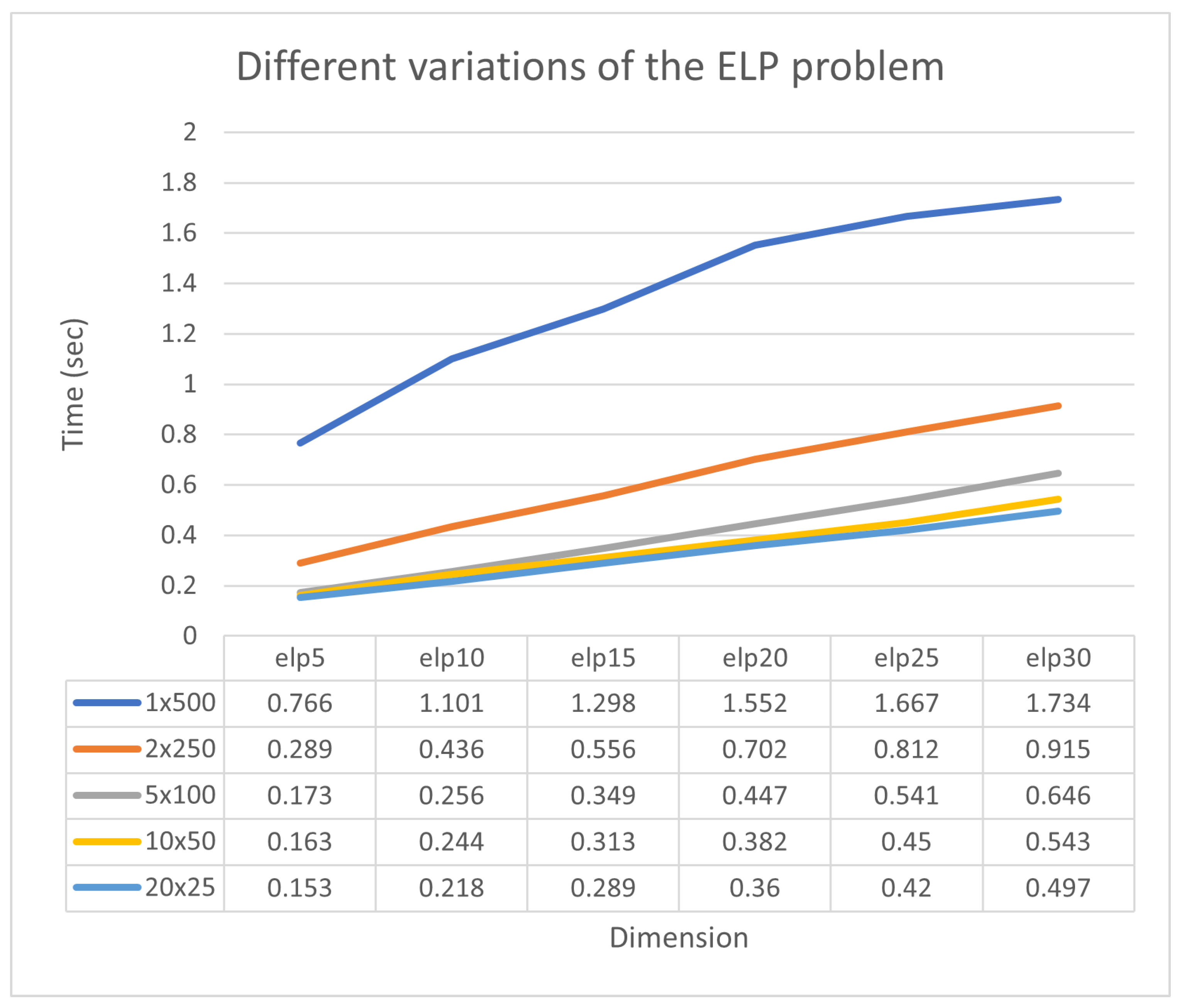
• Sinusoidal function. The function is given by the following:

  $$f\left(x\right)=-\left(2.5\prod _{i=1}^{n}sin\left(x_i-z\right)+\prod _{i=1}^{n}sin\left(5\left(x_i-z\right)\right)\right),0\le x_i\le \pi .$$
  The global minimum is situated at $x^{*}=(2.09435,2.09435,\dots ,2.09435)$ with a value of $f\left(x^{*}\right)=-3.5$. In the performed experiments, we examined scenarios with $n=4,8$ and $z=\frac{\pi }{6}$. The parameter (z) is employed to offset the position of the global minimum [70].
• Test2N function. This function is given by the following equation:

  $$f\left(x\right)=\frac{1}{2}\sum _{i=1}^n{x}_i^4-16x_i^2+5x_i,x_i\in [-5,5].$$
  The function has $2^n$ in the specified range; in our experiments, we used $n=4,5,6,7,8,9$.
• Test30N function. This function is given by the following:

  $$f\left(x\right)=\frac{1}{10}{sin}^2\left(3\pi x_1\right)\sum _{i=2}^{n-1}\left({\left(x_i-1\right)}^2\left(1+{sin}^2\left(3\pi x_{i+1}\right)\right)\right)+{\left(x_n-1\right)}^2\left(1+{sin}^2\left(2\pi x_n\right)\right)$$

  with $x\in [-10,10]$. This function has ${30}^n$ local minima in the specified range, and we used $n=3,4$ in the conducted experiments.

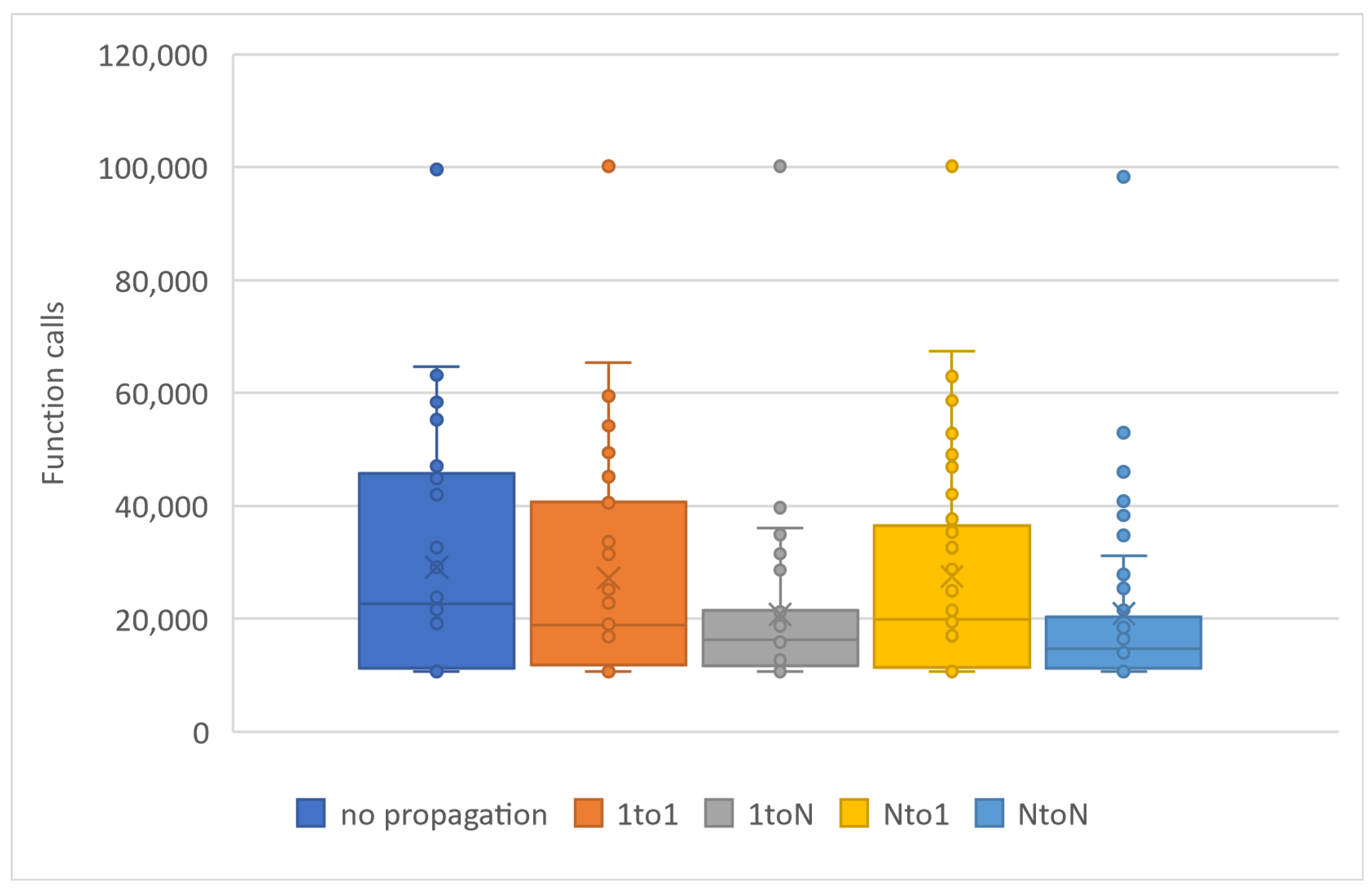
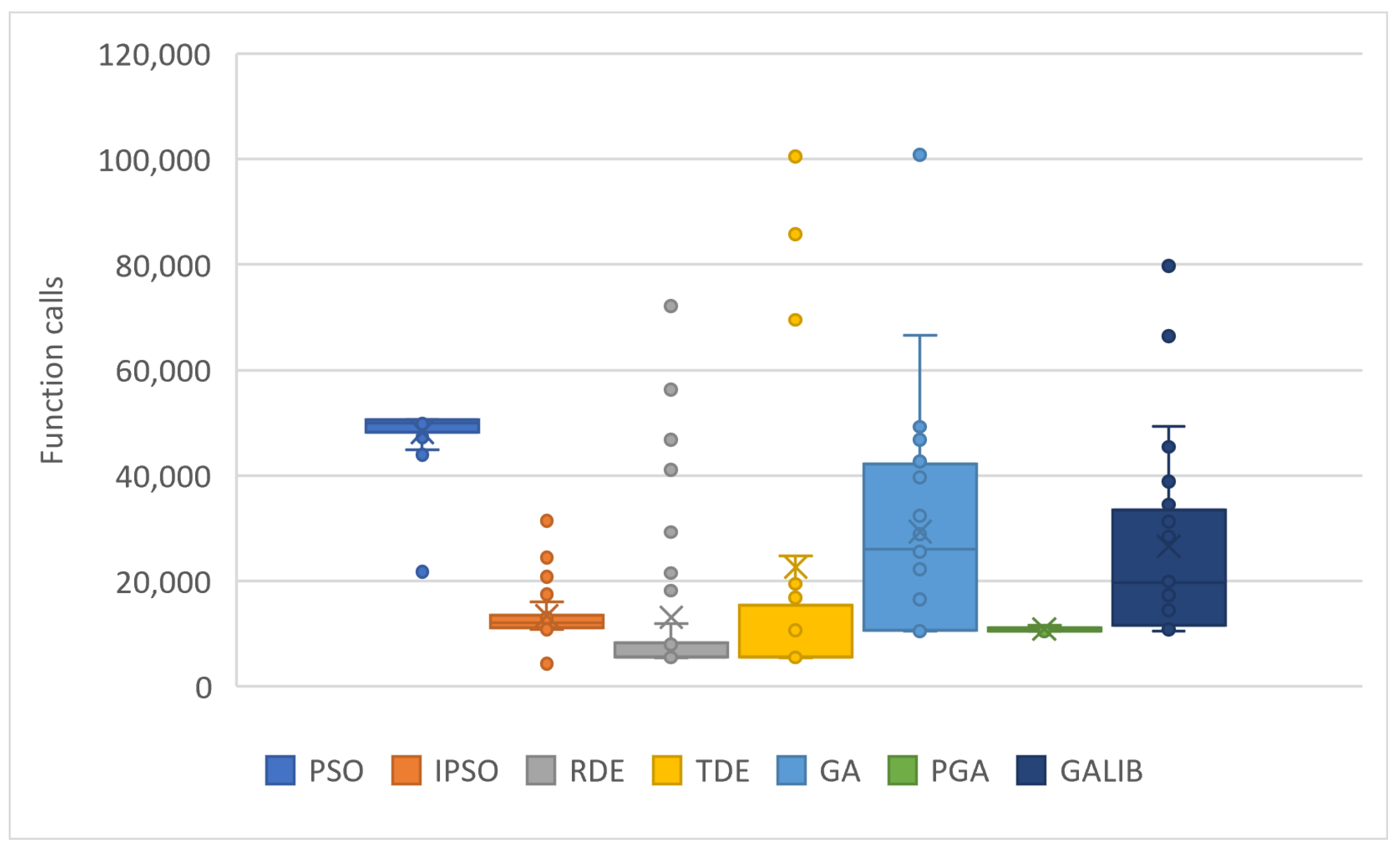
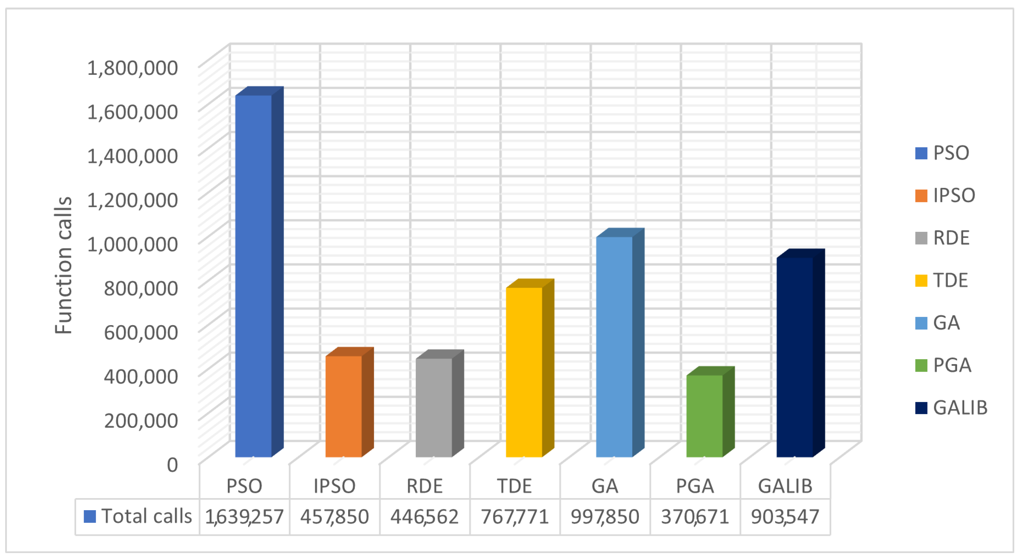
3.2. Experimental Results

To evaluate the performance of the parallel genetic algorithm, a series of experiments were carried out. These experiments varied the number of parallel computing units from 1 to 10. The parallelization was achieved using the freely available OpenMP library [49], and the method was implemented in ANSI C++ within the OPTIMUS optimization package, accessible at https://github.com/itsoulos/OPTIMUS (accessed on 7 June 2024). All experiments were conducted on a system equipped with an AMD Ryzen 5950X processor, 128 GB of RAM, and running the Debian Linux operating system. The experimental settings are shown in

Table 1. The following settings were initially used to conduct the experiments.

Parameter	Value	Explanation
$N_c$	500 × 1, 250 × 2, 100 × 5, 50 × 10	Chromosomes
$N_g$	200	Max generations
$N_I$	1, 2, 5, 10	Processing units or islands
$N_R$	no propagation in Table 2, 1: in every generation in Table 3	Rate of propagation
$N_P$	0 in Table 2, 10: in Table 3	Chromosomes for migration
$PT$	no in Table 2, 1to1 Figure 2a, 1toN Figure 2b, Nto1 Figure 2c, NtoN Figure 2d	Propagation technique
$p_s$	10%	Selection rate
$p_m$	5%	Mutation rate
$LSR$	0.1% in Table 2, 0.5% in Table 3	Local search rate

. To ensure the reliability and validity of the research, experiments were conducted 30 times and concerned

Table 2. Statistical analysis comparing execution times (seconds) and function calls across varying numbers of processor units.

Problems	${\mathit{N}}_{\mathit{i}}=1$ ${\mathit{N}}_{\mathit{c}}=500$ Calls	${\mathit{N}}_{\mathit{i}}=1$ ${\mathit{N}}_{\mathit{c}}=500$ Time	${\mathit{N}}_{\mathit{i}}=2$ ${\mathit{N}}_{\mathit{c}}=250$ Calls	${\mathit{N}}_{\mathit{i}}=2$ ${\mathit{N}}_{\mathit{c}}=250$ Time	${\mathit{N}}_{\mathit{i}}=5$ ${\mathit{N}}_{\mathit{c}}=100$ Calls	${\mathit{N}}_{\mathit{i}}=5$ ${\mathit{N}}_{\mathit{c}}=100$ Time	${\mathit{N}}_{\mathit{i}}=10$ ${\mathit{N}}_{\mathit{c}}=50$ Calls	${\mathit{N}}_{\mathit{i}}=10$ ${\mathit{N}}_{\mathit{c}}=50$ Time
BF1	10,578	0.557	10,555	0.193	10,533	0.126	10,511	0.121
BF2	10,568	0.554	10,545	0.192	10,523	0.127	10,533	0.119
BRANIN	46,793	2.308	31,231	0.562	11,125	0.134	10,533	0.169
CAMEL	26,537	1.338	15,875	0.29	15,833	0.188	10,861	0.123
CIGAR10	10,502	1.089	10,577	0.383	10,583	0.222	10,541	0.206
CM4	10,614	1.054	10,583	0.249	10,581	0.151	10,556	0.139
DISCUS10	10,548	1.09	10,532	0.382	10,500	0.222	10,502	0.205
EASOM	100,762	4.504	100,610	1.66	94,541	1.089	22,845	0.248
ELP10	10,601	1.15	10,590	0.436	10,574	0.26	10,557	0.242
EXP4	16,621	1.092	10,587	0.249	10,560	0.15	10,544	0.143
EXP16	10,680	1.336	10,654	0.53	10,643	0.287	10,626	0.258
EXP64	10,857	2.333	10,829	1.235	10,814	0.825	10,830	0.728
EXP100	10,855	3.517	10,901	1.763	10,868	1.25	10,887	1.052
GKLS250	50,804	2.825	25,832	0.607	11,711	0.194	10,870 (93)	0.198
GKLS350	40,707	2.327	23,720	0.522	17,646	0.26	14,130	0.202
GRIEWANK2	10555	0.565	10532	0.197	10,517	0.126	10,492	0.118
GRIEWANK10	10,679	1.079	10,629	0.407	10,613	0.239	10,609	0.22
POTENTIAL3	39,607	2.057	34,327	0.881	18,313	0.34	15,471	0.279
PONTENTIAL5	33,542	1.653	33737	1.074	12,040	0.34	11,082	0.291
PONTENTIAL6	28,901 (3)	1.56	26,419 (16)	1.018	14,265 (3)	0.478	11,109 (10)	0.356
PONTENTIAL10	42,644 (13)	3.316	37,897 (23)	2.538	14,080 (10)	0.937	11,319 (6)	0.66
HANSEN	46,894 (90)	2.494	28,191 (80)	0.575	11,085 (56)	0.153	11,065	0.158
HARTMAN3	22,235	1.525	19,030	0.379	16,463	0.212	12,048	0.146
HARTMAN6	18,352	1.505	15,902	0.429	16,726	0.279	12,243	0.196
RASTRIGIN	16,567	0.855	10,543	0.193	10,521	0.125	10,506	0.116
ROSENBROCK8	10,863	0.916	10,700	0.333	10,698	0.199	10,772	0.196
POSENBROCK16	10,918	1.371	10946	0.516	10,867	0.304	10,886	0.271
SHEKEL5	32,319 (50)	2.069	17,913 (50)	0.412	11,185 (36)	0.159	11,010 (40)	0.15
SHEKEL7	51,183 (73)	3.277	14,981 (53)	0.342	11,457 (60)	0.163	11,035 (50)	0.154
SHEKEL10	47,337 (70)	2.977	46,927 (76)	1.113	16,310 (56)	0.23	11,329 (70)	0.152
SINU4	66,625 (83)	4.344	31,511 (86)	0.77	13,979 (73)	0.211	11,004 (43)	0.161
SINU8	29,705	2.57	27,613	0.987	24,592	0.549	11,422	0.236
TEST2N4	25,553	1.558	17,701	0.397	24,763	0.359	13,217	0.178
TEST2N5	20,297	1.327	18,440	0.457	16,759	0.265	11,483	0.168
TEST2N6	20,450	1.311	20,837	0.566	18,123	0.315	11,988	0.194
TEST2N7	26,113	1.924	23,940	0.723	20,825	0.384	11,339	0.196
TEST2N8	18,846	1.454	18,549	0.585	16,700	0.329	11,658	0.218
TEST2N9	18,154	1.582	18,803	0.649	17,100	0.368	13,299	0.262
TEST30N3	49,235	2.46	24,129	0.458	14,743	0.188	12,345	0.152
TEST30N4	29,667	1.553	17,501	0.358	13,367	0.186	11,778	0.151
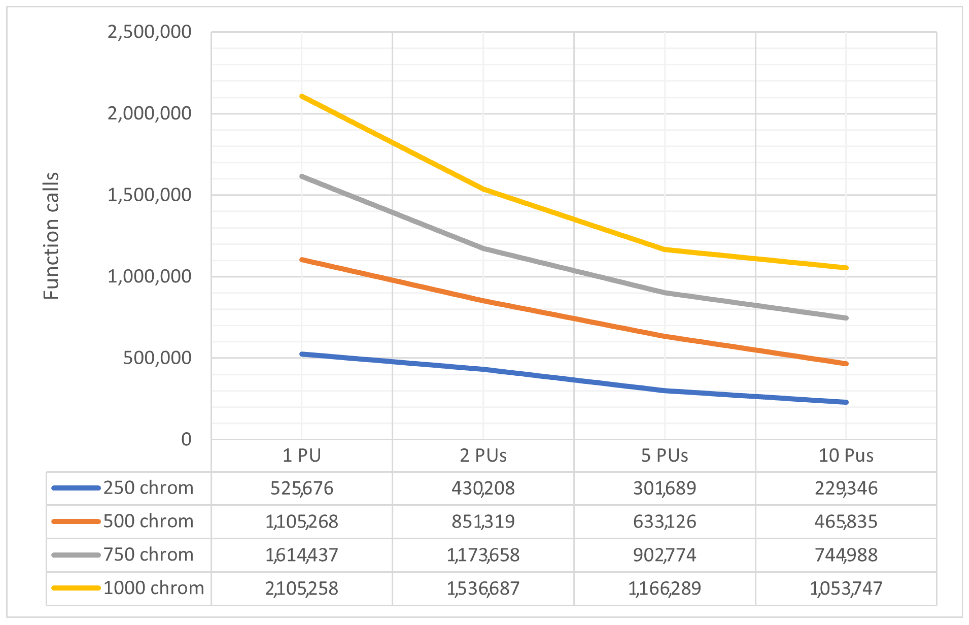
SUM	1,105,268	74.376	851,319	25.61	633,126	12.923	465,835	9.532
MINIMUM	10,502	0.554	10,532	0.192	10,500	0.125	10492	0.116
MAXIMUM	100,762	4.504	100,610	2.538	94,541	1.25	22,845	1.052
AVERAGE	27,631.7	1.859	21,282.975	0.640	15,828.15	0.323	11,645.875	0.238
STDEV	19,305.784	0.972	15,829.020	0.482	13,335.509	0.260	2109.230	0.180

,

Table 3. Evaluating function calls and times (seconds) using various propagation techniques for comparison.

Problems	No Propagation Calls	No Propagation Time	1to1 Calls	1to1 Time	1toN Calls	1toN Time	Nto1 Calls	Nto1 Time	NtoN Calls	NtoN Time
BF1	10,809	0.123	10,741	0.127	10,770	0.126	10,746	0.127	10,808	0.136
BF2	10,725	0.124	10,773	0.126	10,764	0.13	10,783	0.126	10,731	0.136
BRANIN	48,364	0.56	31,470	0.397	18,776	0.251	35,367	0.448	19,224	0.284
CAMEL	29,087	0.337	18,597	0.23	14,429	0.185	24,977	0.313	19,341	0.286
CIGAR10	10,854	0.233	10,880	0.216	10,915	0.222	10,890	0.22	10,869	0.235
CM4	10,911	0.147	10,923	0.15	10,941	0.15	10,918	0.15	10,915	0.163
DISCUS10	10,651	0.222	10,632	0.213	10,651	0.217	10,641	0.22	10,606	0.231
EASOM	99,569	1.094	100,163	1.106	100,160	1.121	100,155	1.139	98,336	1.156
ELP10	10,832	0.276	10,902	0.261	10,829	0.266	10,811	0.26	10,952	0.278
EXP4	10,803	0.151	12,037	0.167	12,695	0.183	11,416	0.164	10,819	0.158
EXP16	11,228	0.272	11,259	0.276	11,262	0.285	11253	0.28	11,260	0.294
EXP64	12,127	0.837	12,204	0.848	12,184	0.85	12,151	0.849	12,199	0.877
EXP100	12,396	1.397	12,376	1.4	12,372	1.36	12,460	1.387	12,414	1.42
GKLS250	48,672	0.813	55,586	0.949	31,493	0.564	58,638	1.007	27,840	0.532
GKLS350	55,231	0.815	42,100	0.636	28,609	0.459	46,923	0.72	25,341	0.428
GRIEWANK2	10,682	0.127	10,670	0.125	10,697	0.126	10,683	0.127	10,684	0.134
GRIEWANK10	11,144	0.239	11,102	0.232	11,123	0.239	11,171	0.229	11,153	0.254
POTENTIAL3	45,748	0.832	33,598	0.643	17,276	0.347	32,603	0.631	16,870	0.358
PONTENTIAL5	41,946	1.156	41,112	1.179	19,912	0.597	37,687	1.089	19,622	0.614
PONTENTIAL6	46,507	1.639	40,518	1.449	21,941	0.817	36,138	1.315	21,528	0.844
PONTENTIAL10	47,031	3.4	45,166	3.361	40,212	3.239	42,057	3.183	34,750	2.883
HANSEN	63,130	0.85	65,414	0.918	39,649	0.595	67,369	0.947	31,149	0.507
HARTMAN3	19,170	0.248	20,339	0.274	16,280	0.226	20,001	0.265	14,587	0.219
HARTMAN6	23,725	0.423	16,856	0.285	14,141	0.233	16,955	0.288	13,964	0.239
RASTRIGIN	11,264	0.147	11,256	0.132	10,652	0.126	10,668	0.128	11,290	0.145
ROSENBROCK8	11,727	0.204	11,892	0.2	11,681	0.203	11,708	0.199	11,882	0.217
POSENBROCK16	12372	0.42	12,187	0.304	12,394	0.313	12,438	0.324	12,455	0.324
SHEKEL5	44,893	0.645	54,184	0.751	34,937	0.491	53,277	0.755	40,859	0.621
SHEKEL7	45,722	0.638	55,109	0.778	33,440	0.472	49,029	0.702	46,066	0.696
SHEKEL10	58,361	0.854	49,400	0.721	32,691	0.471	52,798	0.783	38,305	0.608
SINU4	64,584	0.972	59,414	0.922	36,052	0.591	62,924	0.972	52,937	0.857
SINU8	32,572	0.793	25,552	0.63	19,461	0.462	28,744	0.716	18,173	0.445
TEST2N4	23,430	0.339	20,474	0.3	17,001	0.261	21,468	0.316	18,436	0.294
TEST2N5	22,662	0.358	20,614	0.33	16,171	0.262	19,697	0.316	16,421	0.282
TEST2N6	21,663	0.365	18,721	0.323	16,600	0.289	19,556	0.339	14,633	0.299
TEST2N7	24,401	0.456	18,990	0.354	15,792	0.3	20,967	0.405	13,995	0.28
TEST2N8	21,017	0.418	18,532	0.369	16,644	0.339	20,139	0.413	13,980	0.298
TEST2N9	22,684	0.488	18,538	0.407	16302	0.353	18,929	0.421	14,620	0.344
TEST30N3	24,524	0.318	22,799	0.296	20,436	0.297	23,186	0.311	19,968	0.316
TEST30N4	21,090	0.28	25,160	0.358	21,216	0.319	19,444	0.276	16,711	0.267
Total	1,164,308	24.01	1,088,240	22.74	829,551	18.33	1,097,765	22.86	836,693	18.95

and

Table 4. Comparison of function calls using different stochastic optimization methods.

PROBLEMS	PSO	IPSO	RDE	TDE	GA	GAlib	PGA
BF1	50,398	11,478	7943 (86)	5535	10,578	11,641	10,501
BF2	50,397	11,292	8472 (76)	5539	10,568	11,321	10,510
BRANIN	44,800	10,849	5513	5514	46,793	34,487	10,838
CAMEL	48,242	11,051	5555	5514	26,537	17,321	11,087
CIGAR10	50,581	12,331	5586	100,573	10,502	11,567 (50)	10,566
CM4	48,559	11,767	5550	5538	10,614	11,118 (70)	10,548
DISCUS10	50,523	14,328	18,187	100,518	10,548	10,988	10,503
EASOM	21,786	10,938	29,256	24,691	100,762	79,689	10,797
ELP10	49,837	4323	11,933	100,584	10,601	11,673	10,559
EXP4	48,523	11,041	46,752	19,467	16,621	16,045	10,503
EXP16	50,518	10,973	5537	69,494	10,680	10,500	10,595
GKLS250	43,925	10,869	41,016	11,430	50,804	31,298	10,893 (76)
GKLS350	48,202	10,750	56,220	16,831	40,707	29,897 (96)	11,555 (96)
GRIEWANK2	44,021	13,514	5538	5533	10,555	14,419 (67)	10,498
GRIEWANK10	50,557 (3)	12,258 (86)	5612 (13)	85,742 (3)	10,679	10,800	10,576
POTENTIAL3	49,213	12,124	5530	5523	39,607	33,452	11,039
PONTENTIAL5	50,548	16,027	5587	5569	33,542	31,285	11,134
PONTENTIAL6	50,558 (3)	24,414 (66)	5607 (6)	5588 (3)	28,901 (3)	28,444 (10)	11,143 (10)
PONTENTIAL10	50,641 (6)	31,434	5670 (3)	5661 (6)	42,644 (13)	38,883 (20)	11,290 (20)
HANSEN	47,296	13,131	5522	5521	46,894 (90)	45,440	11,055
HARTMAN3	47,778	10,961	5525	5522	22,235	19,434	11,097
HARTMAN6	50,088 (33)	11,085 (86)	5536 (83)	5536	18,352	18,444 (60)	11,273
RASTRIGIN	47,433	11,594	5542	5524	16,567	16,286 (96)	10,506
ROSENBROCK8	50,549	13,487	72,088	100,503	10,863	11,419	10,645
POSENBROCK16	50,584	12,659	21,517	10,645	10,918	11,681	10,957
SHEKEL5	49,944 (33)	13,058 (93)	5532 (86)	5524 (93)	32,319 (50)	29,287	10,883 (43)
SHEKEL7	50,062 (53)	12,134 (96)	5533 (96)	5523	51183 (73)	47,245 (77)	10,926 (53)
SHEKEL10	50,124 (63)	14,176	5535 (90)	5523	47,337 (70)	45,911 (77)	11,207 (80)
SINU4	49,239	11,349	5527	5510	66,625 (83)	66,383	11,063 (76)
SINU8	50,224	11,295	5537 (80)	5520	29,705	29,234	11,378
TEST2N4	50,112 (93)	13,173	5529	5519	25,553	19,913	11049
TEST2N9	50,517 (13)	17,510 (60)	5546 (6)	5535 (56)	18,154	15,376	11,145
TEST30N3	44,301	19,638	5515	5511	49,235	49,234	11,051
TEST30N4	49,177	20,839	5514	5511	29,667	33,428	11,301
TOTAL	1,639,257	457,850	446,562	767,771	997,850	903,547	370,671

. In Table 2, the number of objective function invocations for each problem and its solving time for various combinations of processing units (PUs) and chromosomes are provided. In the columns listing objective function invocation values, values in parentheses represent the percentage of executions where the overall optimum was successfully identified. The absence of this fraction indicates a 100% success rate, meaning that the global minimum was found in every run. Generally, across all problems, there is a decrease in the number of objective function invocations and execution time as the number of parallel computing units increases. The number of chromosomes remains constant in each case, e.g., 1PUx500chrom, 2PUx250chrom, etc. This is a positive result, indicating that parallelization improves the performance of the genetic algorithm. Figure 3 and Figure 4 are derived from Table 2. A statistical comparison of objective function invocations, solving times, and execution times similarly shows performance improvements and computation time reductions for problems as the number of computing units increases.

Specifically, in Figure 3, the objective function invocations are halved compared to the initial invocations with only two computational units. This reduction in invocations continues significantly as the number of computational units increases. In Figure 4, we observe similar behavior in the algorithm termination times. In this case, the times are significantly shorter in the parallel process with ten (10) computational units compared to a single computational unit. In the comparisons presented above, there is a reduction in the required computational power, as shown in Figure 3, along with a decrease in the time required to find solutions, as depicted in Figure 4. In Table 2, additional interesting details regarding objective function invocations and computational times are presented, such as minimum, maximum, mean, and standard deviations. In conclusion, as the workload is distributed among an increasing number of computational units, there is a performance improvement. This reinforces the overall methodology.

In Table 3, chromosome migration with the best functional values occurs in every generation, involving a specific number of ten chromosomes, N P = 10, participating in the propagation process. To enhance the implementation of propagation techniques, we increased the local optimization rate applied in Table 3 from 0.1% (as presented in Table 2) to 0.5% LSR. However, the level of local optimization was carefully controlled because an excessive increase could lead to a higher number of calls to the objective function. Conversely, reducing the LSR might lead to a decrease in the success rate concerning the identification of optimal chromosomes. In the statistical representation of Figure 5, we observe the superiority of the ‘1 to N’ propagation, meaning the transfer of ten chromosomes from a random island to all others. The ’N to N’ propagation appears to be equally effective. As a general rule, if we classify migration methods based on their performance, they will be ranked as follows: ‘1toN’ in Figure 2b, ‘NtoN’ in Figure 2d, ‘1to1’ in Figure 2a, and ’Nto1’ in Figure 2c. The first two strategies, where migration occurs across all islands, demonstrate better performance compared to the other two, where migration only affects one island. The success of ‘1toN’ in Figure 2b and ‘NtoN’ in Figure 2d, albeit with a slight difference, appears to be due to the migration of the best chromosomes to all islands. This leads to an improvement in the convergence of the algorithm towards better candidate solutions in a shorter time frame. The actual times are shown in Figure 6. During the conducted experiments, the “1-to-N” and “N-to-N” propagation techniques appear to perform better according to experimental evidence. A common feature of these two techniques is that the optimal solutions are distributed to all computing units, thereby improving the performance of each individual unit and consequently enhancing the overall performance of the general algorithm.

To conduct experiments among stochastic methods of global optimization, including particle swarm optimization (PSO), improved PSO (IPSO) [71], differential evolution with random selection (DE), differential evolution with tournament selection (TDE) [72], genetic algorithm (GA), and parallel genetic algorithm (PGA), certain parameters remained constant. Also, the parallel implementation of the GAlib library [73] was used in the comparative experiments. The population size for all consists of 500 particles, agents, or chromosomes. In PGA, the population consists of 20PU × 25chrom, while all other parameters remain the same as those described in Table 2. Any method employing LSR maintains this parameter at the same value. The double box is a termination rule that is consistent across all methods.

The values resulting from experiments in Table 4 are depicted in Figure 7 and Figure 8. The box plots of Figure 7 reveal the superiority of PGA, as the number of objective function calls remains at approximately 10,000 across all problems. Conversely, IPSO, DE, and TDE (especially DE) show a low number of calls in some problems, while in others, they experience significant increases. Each method has a specific lower limit of calls during initialization and optimization, which varies from method to method. PGA consistently meets this threshold with very small deviations, as illustrated in the same figure. Figure 8 presents the total call values for each method. This work was also compared against the parallel version of GAlib, found in recent literature. Although GAlib achieves a similar success rate in discovering the global minimum of the benchmark functions, it requires significantly more function calls than the proposed method for the same setup parameters.

In Figure 9, it is observed that the collaboration of sub-listing units significantly accelerates the process of finding minima. Additionally, a new experiment was conducted where the number of chromosomes varied from 250 to 1000 and the number of processing units changed from 1 to 10. The total number of function calls for each case is graphically shown in Figure 10. The method maintains the same behavior for any number of chromosomes. This means that the set of required calls is significantly reduced by adding new parallel processing units. Of course, as expected, the total number of calls required increases as the number of available chromosomes increases.

4. Conclusions

According to the relevant literature, despite the high success rate that genetic algorithms exhibit in finding good functional values, they require significant computational power, leading to longer processing times. This manuscript introduces a parallel technique for global optimization, employing a genetic algorithm to solve the problem. Specifically, the initial population of chromosomes is divided into various subpopulations that run on different computational units. During the optimization process, the islands operate independently but periodically exchange chromosomes with good functional values. The number of chromosomes participating in migration is determined by the crossover and mutation rates. Additionally, periodic local optimization is performed on each computational unit, which should not require excessive computational power (function calls).

Experimental results revealed that even parallelization with just two computational units significantly reduces both the number of function calls and processing time, proving to be quite effective even with more computational units. Furthermore, it was observed that the most effective information exchange technique was the so-called ‘1toN’, with a slight difference from the ‘NtoN’, where a randomly selected subpopulation sends information to all other subpopulations. Moreover, the ‘NtoN’ technique—where all subpopulations send information to all other subpopulations—seems to perform equally well.

Similar dissemination techniques have been applied to other stochastic methods, such as the differential evolution (DE) method by Charilogis and Tsoulos [74] and the particle swarm optimization (PSO) method by Charilogis and Tsoulos [75]. In the case of differential evolution, the proposed dissemination technique is ‘1to1’ in Figure 2a and not ‘1toN’ in Figure 2b as suggested in this study. However, in the case of PSO and GA, the recommended dissemination technique is the same.

The parallelization of various methodologies of genetic algorithms or even different stochastic techniques for global optimization can be explored to enhance the methodology. However, in such heterogeneous environments, more efficient termination criteria are required, or even their combined use may be necessary.

References

- Törn, A.; Žilinskas, A. Global Optimization; Springer: Berlin/Heidelberg, Germany, 1989; Volume 350, pp. 1–255. [Google Scholar]
- Fouskakis, D.; Draper, D. Stochastic optimization: A review. Int. Stat. Rev. 2002, 70, 315–349. [Google Scholar] [CrossRef]
- Cherruault, Y. Global optimization in biology and medicine. Math. Comput. Model. 1994, 20, 119–132. [Google Scholar] [CrossRef]
- Lee, E.K. Large-Scale Optimization-Based Classification Models in Medicine and Biology. Ann. Biomed. Eng. 2007, 35, 1095–1109. [Google Scholar] [CrossRef]
- Liwo, A.; Lee, J.; Ripoll, D.R.; Pillardy, J.; Scheraga, H.A. Protein structure prediction by global optimization of a potential energy function. Biophysics 1999, 96, 5482–5485. [Google Scholar] [CrossRef] [PubMed]
- Shin, W.H.; Kim, J.K.; Kim, D.S.; Seok, C. GalaxyDock2: Protein-ligand docking using beta-complex and global optimization. J. Comput. Chem. 2013, 34, 2647–2656. [Google Scholar] [CrossRef] [PubMed]
- Duan, Q.; Sorooshian, S.; Gupta, V. Effective and efficient global optimization for conceptual rainfall-runoff models. Water Resour. Res. 1992, 28, 1015–1031. [Google Scholar] [CrossRef]
- Yang, L.; Robin, D.; Sannibale, F.; Steier, C.; Wan, W. Global optimization of an accelerator lattice using multiobjective genetic algorithms, Nuclear Instruments and Methods in Physics Research Section A: Accelerators, Spectrometers. Detect. Assoc. Equip. 2009, 609, 50–57. [Google Scholar] [CrossRef]
- Iuliano, E. Global optimization of benchmark aerodynamic cases using physics-based surrogate models. Aerosp. Sci. Technol. 2017, 67, 273–286. [Google Scholar] [CrossRef]
- Maranas, C.D.; Androulakis, I.P.; Floudas, C.A.; Berger, A.J.; Mulvey, J.M. Solving long-term financial planning problems via global optimization. J. Econ. Dyn. Control 1997, 21, 1405–1425. [Google Scholar] [CrossRef]
- Gaing, Z. Particle swarm optimization to solving the economic dispatch considering the generator constraints. IEEE Trans. Power Syst. 2003, 18, 1187–1195. [Google Scholar] [CrossRef]
- Liberti, L.; Kucherenko, S. Comparison of deterministic and stochastic approaches to global optimization. Int. Trans. Oper. Res. 2005, 12, 263–285. [Google Scholar] [CrossRef]
- Wolfe, M.A. Interval methods for global optimization. Appl. Math. Comput. 1996, 75, 179–206. [Google Scholar] [CrossRef]
- Csendes, T.; Ratz, D. Subdivision Direction Selection in Interval Methods for Global Optimization. SIAM J. Numer. Anal. 1997, 34, 922–938. [Google Scholar] [CrossRef]
- Maranas, C.D.; Floudas, C.A. A deterministic global optimization approach for molecular structure determination. J. Chem. Phys. 1994, 100, 1247. [Google Scholar] [CrossRef]
- Barhen, J.; Protopopescu, V.; Reister, D. TRUST: A Deterministic Algorithm for Global Optimization. Science 1997, 276, 1094–1097. [Google Scholar] [CrossRef]
- Evtushenko, Y.; Posypkin, M.A. Deterministic approach to global box-constrained optimization. Optim. Lett. 2013, 7, 819–829. [Google Scholar] [CrossRef]
- Dorigo, M.; Birattari, M.; Stutzle, T. Ant colony optimization. IEEE Comput. Intell. Mag. 2006, 1, 28–39. [Google Scholar] [CrossRef]
- Socha, K.; Dorigo, M. Ant colony optimization for continuous domains. Eur. J. Oper. Res. 2008, 185, 1155–1173. [Google Scholar] [CrossRef]
- Price, W.L. Global optimization by controlled random search. J. Optim. Theory Appl. 1983, 40, 333–348. [Google Scholar] [CrossRef]
- Křivý, I.; Tvrdík, J. The controlled random search algorithm in optimizing regression models. Comput. Stat. Data Anal. 1995, 20, 229–234. [Google Scholar] [CrossRef]
- Ali, M.M.; Törn, A.; Viitanen, S. A Numerical Comparison of Some Modified Controlled Random Search Algorithms. J. Glob. Optim. 1997, 11, 377–385. [Google Scholar] [CrossRef]
- Kennedy, J.; Eberhart, R. Particle swarm optimization. In Proceedings of the ICNN’95—International Conference on Neural Networks, Perth, WA, Australia, 27 November–1 December 1995; Volume 4, pp. 1942–1948. [Google Scholar] [CrossRef]
- Trelea, I.C. The particle swarm optimization algorithm: Convergence analysis and parameter selection. Inf. Process. Lett. 2003, 85, 317–325. [Google Scholar] [CrossRef]
- Poli, R.; Kennedy, J.; Blackwell, T. Particle swarm optimization An Overview. Swarm Intell. 2007, 1, 33–57. [Google Scholar] [CrossRef]
- Kirkpatrick, S.; Gelatt, C.D.; Vecchi, M.P. Optimization by simulated annealing. Science 1983, 220, 671–680. [Google Scholar] [CrossRef] [PubMed]
- Ingber, L. Very fast simulated re-annealing. Math. Comput. Model. 1989, 12, 967–973. [Google Scholar] [CrossRef]
- Eglese, R.W. Simulated annealing: A tool for operational research. Eur. J. Oper. Res. 1990, 46, 271–281. [Google Scholar] [CrossRef]
- Storn, R.; Price, K. Differential Evolution—A Simple and Efficient Heuristic for Global Optimization over Continuous Spaces. J. Glob. Optim. 1997, 11, 341–359. [Google Scholar] [CrossRef]
- Liu, J.; Lampinen, J. A Fuzzy Adaptive Differential Evolution Algorithm. Soft Comput. 2005, 9, 448–462. [Google Scholar] [CrossRef]
- Goldberg, D. Genetic Algorithms in Search, Optimization and Machine Learning; Addison-Wesley Publishing Company: Reading, MA, USA, 1989. [Google Scholar]
- Michaelewicz, Z. Genetic Algorithms + Data Structures = Evolution Programs; Springer: Berlin/Heidelberg, Germany, 1996. [Google Scholar]
- Grady, S.A.; Hussaini, M.Y.; Abdullah, M.M. Placement of wind turbines using genetic algorithms. Renew. Energy 2005, 30, 259–270. [Google Scholar] [CrossRef]
- Lepagnot, I.B.J.; Siarry, P. A survey on optimization metaheuristics. Inf. Sci. 2013, 237, 82–117. [Google Scholar]
- Dokeroglu, T.; Sevinc, E.; Kucukyilmaz, T.; Cosar, A. A survey on new generation metaheuristic algorithms. Comput. Ind. Eng. 2019, 137, 106040. [Google Scholar] [CrossRef]
- Hussain, K.; Salleh, M.N.M.; Cheng, S.; Shi, Y. Metaheuristic research: A comprehensive survey. Artif. Intell. Rev. 2019, 52, 2191–2233. [Google Scholar] [CrossRef]
- Holland, J.H. Genetic algorithms. Sci. Am. 1992, 267, 66–73. [Google Scholar] [CrossRef]
- Stender, J. Parallel Genetic Algorithms: Theory & Applications; IOS Press: Amsterdam, The Netherlands, 1993. [Google Scholar]
- Santana, Y.H.; Alonso, R.M.; Nieto, G.G.; Martens, L.; Joseph, W.; Plets, D. Indoor genetic algorithm-based 5G network planning using a machine learning model for path loss estimation. Appl. Sci. 2022, 12, 3923. [Google Scholar] [CrossRef]
- Liu, X.; Jiang, D.; Tao, B.; Jiang, G.; Sun, Y.; Kong, J.; Chen, B. Genetic algorithm-based trajectory optimization for digital twin robots. Front. Bioeng. Biotechnol. 2022, 9, 793782. [Google Scholar] [CrossRef] [PubMed]
- Nonoyama, K.; Liu, Z.; Fujiwara, T.; Alam, M.M.; Nishi, T. Energy-efficient robot configuration and motion planning using genetic algorithm and particle swarm optimization. Energies 2022, 15, 2074. [Google Scholar] [CrossRef]
- Liu, K.; Deng, B.; Shen, Q.; Yang, J.; Li, Y. Optimization based on genetic algorithms on energy conservation potential of a high speed SI engine fueled with butanol–Gasoline blends. Energy Rep. 2022, 8, 69–80. [Google Scholar] [CrossRef]
- Zhou, G.; Zhu, Z.; Luo, S. Location optimization of electric vehicle charging stations: Based on cost model and genetic algorithm. Energy 2022, 247, 123437. [Google Scholar] [CrossRef]
- Min, D.; Song, Z.; Chen, H.; Wang, T.; Zhang, T. Genetic algorithm optimized neural network based fuel cell hybrid electric vehicle energy management strategy under start-stop condition. Appl. Energy 2022, 306, 118036. [Google Scholar] [CrossRef]
- Doewes, R.I.; Nair, R.; Sharma, T. Diagnosis of COVID-19 through blood sample using ensemble genetic algorithms and machine learning classifier. World J. Eng. 2022, 19, 175–182. [Google Scholar] [CrossRef]
- Choudhury, S.; Rana, M.; Chakraborty, A.; Majumder, S.; Roy, S.; RoyChowdhury, A.; Datta, S. Design of patient specific basal dental implant using Finite Element method and Artificial Neural Network technique. J. Eng. Med. 2022, 236, 1375–1387. [Google Scholar] [CrossRef] [PubMed]
- Chen, Q.; Hu, X. Design of intelligent control system for agricultural greenhouses based on adaptive improved genetic algorithm for multi-energy supply system. Energy Rep. 2022, 8, 12126–12138. [Google Scholar] [CrossRef]
- Graham, R.L.; Woodall, T.S.; Squyres, J.M. Open MPI: A flexible high performance MPI. In Proceedings of the Parallel Processing and Applied Mathematics: 6th International Conference (PPAM 2005), Poznań, Poland, 11–14 September 2005; Revised Selected Papers 6. Springer: Berlin/Heidelberg, Germany, 2006; pp. 228–239. [Google Scholar]
- Ayguadé, E.; Copty, N.; Duran, A.; Hoeflinger, J.; Lin, Y.; Massaioli, F.; Zhang, G. The design of OpenMP tasks. IEEE Trans. Parallel Distrib. Syst. 2008, 20, 404–418. [Google Scholar] [CrossRef]
- Onbaşoğlu, E.; Özdamar, L. Parallel simulated annealing algorithms in global optimization. J. Glob. Optim. 2001, 19, 27–50. [Google Scholar] [CrossRef]
- Schutte, J.F.; Reinbolt, J.A.; Fregly, B.J.; Haftka, R.T.; George, A.D. Parallel global optimization with the particle swarm algorithm. Int. J. Numer. Methods Eng. 2004, 61, 2296–2315. [Google Scholar] [CrossRef] [PubMed]
- Regis, R.G.; Shoemaker, C.A. Parallel stochastic global optimization using radial basis functions. J. Comput. 2009, 21, 411–426. [Google Scholar] [CrossRef]
- Harada, T.; Alba, E. Parallel Genetic Algorithms: A Useful Survey. ACM Comput. Surv. 2020, 53, 86. [Google Scholar] [CrossRef]
- Anbarasu, L.A.; Narayanasamy, P.; Sundararajan, V. Multiple molecular sequence alignment by island parallel genetic algorithm. Curr. Sci. 2000, 78, 858–863. [Google Scholar]
- Tosun, U.; Dokeroglu, T.; Cosar, C. A robust island parallel genetic algorithm for the quadratic assignment problem. Int. Prod. Res. 2013, 51, 4117–4133. [Google Scholar] [CrossRef]
- Nandy, A.; Chakraborty, D.; Shah, M.S. Optimal sensors/actuators placement in smart structure using island model parallel genetic algorithm. Int. J. Comput. 2019, 16, 1840018. [Google Scholar] [CrossRef]
- Tsoulos, I.G.; Tzallas, A.; Tsalikakis, D. PDoublePop: An implementation of parallel genetic algorithm for function optimization. Comput. Phys. Commun. 2016, 209, 183–189. [Google Scholar] [CrossRef]
- Shonkwiler, R. Parallel genetic algorithms. In ICGA; Morgan Kaufmann Publishers Inc: San Francisco, CA, USA, 1993; pp. 199–205. [Google Scholar]
- Cantú-Paz, E. A survey of parallel genetic algorithms. Calc. Paralleles Reseaux Syst. Repartis 1998, 10, 141–171. [Google Scholar]
- Mühlenbein, H. Parallel genetic algorithms in combinatorial optimization. In Computer Science and Operations Research; Elsevier: Amsterdam, The Netherlands, 1992; pp. 441–453. [Google Scholar]
- Lawrence, D. Handbook of Genetic Algorithms; Thomson Publishing Group: London, UK, 1991. [Google Scholar]
- Yu, X.; Gen, M. Introduction to Evolutionary Algorithms; Springer: Berlin/Heidelberg, Germany, 2010; ISBN 978-1-84996-128-8. e-ISBN 978-1-84996-129-5. [Google Scholar] [CrossRef]
- Kaelo, P.; Ali, M.M. Integrated crossover rules in real coded genetic algorithms. Eur. J. Oper. Res. 2007, 176, 60–76. [Google Scholar] [CrossRef]
- Tsoulos, I.G. Modifications of real code genetic algorithm for global optimization. Appl. Math. Comput. 2008, 203, 598–607. [Google Scholar] [CrossRef]
- Powell, M.J.D. A Tolerant Algorithm for Linearly Constrained Optimization Calculations. Math. Program. 1989, 45, 547–566. [Google Scholar] [CrossRef]
- Floudas, C.A.; Pardalos, P.M.; Adjiman, C.; Esposoto, W.; Gümüs, Z.; Harding, S.; Klepeis, J.; Meyer, C.; Schweiger, C. Handbook of Test Problems in Local and Global Optimization; Kluwer Academic Publishers: Dordrecht, The Netherlands, 1999. [Google Scholar]
- Ali, M.M.; Khompatraporn, C.; Zabinsky, Z.B. A Numerical Evaluation of Several Stochastic Algorithms on Selected Continuous Global Optimization Test Problems. J. Glob. Optim. 2005, 31, 635–672. [Google Scholar] [CrossRef]
- Gaviano, M.; Ksasov, D.E.; Lera, D.; Sergeyev, Y.D. Software for generation of classes of test functions with known local and global minima for global optimization. ACM Trans. Math. Softw. 2003, 29, 469–480. [Google Scholar] [CrossRef]
- Lennard-Jones, J.E. On the Determination of Molecular Fields. Proc. R. Soc. Lond. A 1924, 106, 463–477. [Google Scholar]
- Zabinsky, Z.B.; Graesser, D.L.; Tuttle, M.E.; Kim, G.I. Global optimization of composite laminates using improving hit and run. In Recent Advances in Global Optimization; Princeton University Press: Princeton, NJ, USA, 1992; pp. 343–368. [Google Scholar]
- Charilogis, V.; Tsoulos, I. Toward an Ideal Particle Swarm Optimizer for Multidimensional Functions. Information 2022, 13, 217. [Google Scholar] [CrossRef]
- Charilogis, V.; Tsoulos, I.; Tzallas, A.; Karvounis, E. Modifications for the Differential Evolution Algorithm. Symmetry 2022, 14, 447. [Google Scholar] [CrossRef]
- Wall, M. GAlib: A C++ Library of Genetic Algorithm Components; Mechanical Engineering Department, Massachusetts Institute of Technology: Cambridge, MA, USA, 1996; p. 54. [Google Scholar]
- Charilogis, V.; Tsoulos, I.G. A Parallel Implementation of the Differential Evolution Method. Analytics 2023, 2, 17–30. [Google Scholar] [CrossRef]
- Charilogis, V.; Tsoulos, I.G.; Tzallas, A. An Improved Parallel Particle Swarm Optimization. Comput. Sci. 2023, 4, 766. [Google Scholar] [CrossRef]