Abstract
This paper describes various selected properties and features of negative binomial (NB) random variables, with special reference to NB2 (i.e., p = 2), and some generalizations to NBp (i.e., p ≥ 2), specifications. It presents new results (e.g., the NBp moment-generating function) with regard to the relationship between a sample mean and its accompanying variance, as well as spatial statistical/econometric numerical and empirical examples, whose parameter estimators are maximum likelihood or method of moment ones. Finally, it highlights the Moran eigenvector spatial filtering methodology within the context of generalized linear modeling, demonstrating it in terms of spatial negative binomial regression. Its overall conclusion is a bolstering of important findings the literature already reports with a newly recognized empirical example of an NB3 phenomenon.
1. Introduction
Many contemporary random variables (RVs) measure counts (with a zero to infinity support), implying that they are Poisson variates, but without equi-dispersion (i.e., a violation of the μ = σ2 property, most often such that μ < σ2), further implying that their best distributional description is a Poisson variable with a gamma-distributed mean (i.e., a gamma–Poisson mixture), which translates nicely into a negative binomial (NB) RV. However, a standard NB does not always successfully account for this mean–variance discrepancy in such circumstances. Cameron and Trivedi [1] introduce a generalized version of the NB probability model now known as the NBp model, where p is a positive integer, whose goal is to better capture under/over-dispersion; this variate differs from the negative binomial process (NBP) model (e.g., [2]). The literature contains little discussion about this former generalized model, with the exception of Cameron and Trivedi’s initial treatment of it and papers by Greene [3] and by Di et al. [4]. Of note is that an R package (version ≥ 3.00) exists for implementing this model [4]. The purpose of this paper is to address this gap in the literature by (1) clarifying/correcting several misleading technical details in part of Greene’s paper; (2) presenting new results; (3) illuminating selected small and large sample properties on NB models; and (4) presenting new empirical spatial statistics/econometrics instances involving spatial autocorrelation (SA).
A parametric mixture conceptualization—analogous to a Bayesian conjugate prior formulation—is the context of this discussion: the NB specification describes a count’s variable Y that is Poisson distributed, with its mean μ being gamma distributed rather than constant. Accordingly, the gamma RV has parameters αμ2–p and μp–1/α, where μ denotes its mean and 1/α denotes its dispersion parameter, yielding a global NBp model with parameters r = αμ2–p and probability p = 1/(1 + μp–1/α) for some non-negative integer p > 0; p = 1, 2 are standard NB specifications, with the former being the Poisson RV and the latter being the popular NB2 variate.
2. Materials and Methods: Clarifying Greene’s Presentation
Confusing equations appearing in Greene [1] include (2-13) and (2-14), particularly when one contrasts them with his appendix equation (A-2) with regard to the p exponent. In addition, this latter equation is missing a subscript i on the λ variable appearing in the numerator of its third term on its right-hand side. Discussion pertaining to equations (2-4) and (2-5) would be clearer if the posited gamma distribution is stated in its standard symbology as Γ(θ, 1/θ). Greene’s equations (2-13)—in which he incorrectly states q = 1/1(1 + θ) rather than q = 1/(1 + 1/θ)—and (2-14)—in which he states s = λ/(λ + θλ2–p) rather than 1/(1 + μp–2/α)—yield, for independent and identically distributed (iid) NBps, the following probability mass function:
where, adopting more typical literature-appearing notation (particularly for gamma–Poisson specifications) in this paper, μ (denoting the mean) is equivalent to λ and α is the same as θ in Greene’s paper, the subscripts i are not used in this version because it represents a global equation, and the ratio of gamma functions term also can be rewritten employing combinatorial binomial coefficients. The difference is that Greene’s equation (2-14) has an exponent of (2–p) rather than (p–2). Equation (1) renders the revised results of
Greene’s equation (2-14) specification renders
which is not his equation (2-15), even for the specific standard case of p = 2. His probability mass function should be Equation (1), rather than
which is neither the result for a Poisson parametric mixture probability defined by Prob(y) = e−μμy/(y!) with μ ~ Γ(αμ2–p, μp–1/α), nor the outcome from Greene’s replacing α with αμ2–p in this mixture, which renders E(Y) = μ and E[(Y − μ)2] = μ(1 + μp–3/α).
E(Y) = μ and E[(Y − μ)2] = μ(1 + μp–1/α).
3. Results: Articulating NBp Variates
Both mathematical statistics analytical results and simulation experimental output help establish an understanding of a generalization of NB1 and NB2 to NBp. This section furnishes some of each.
3.1. The NBp Moment-Generating Function and Asymptotic Normality
Particularly because the method of moments is a useful estimation technique for parameter α [5], knowing the moments of the NBp specification is desirable. The absence of closed-form maximum likelihood estimators (MLEs, e.g., see [6,7,8,9,10]) makes this ensuing invention even more appealing.
3.1.1. The NBp Moment-Generating Function (mgf)
The NBp mgf is
with the first moment about the origin being
and, hence, the moments about the mean mgf being
The second moment about the mean is μ(1 + μp–1/α).
3.1.2. Asymptotic Normality and an NBp RV
Matching moments is one way to establish equivalency between distributions [11]. Skewness and kurtosis involve the third and fourth moments about the mean, which are derivable from Equation (3), such that for an NBp RV
The Poisson skewness term, , is visible in this preceding first expression. Here, skewness does not necessarily converge on zero, and kurtosis does not necessarily converge on 3, unless the over-dispersion parameter, 1/α, as well as p exhibit certain behaviors and/or properties. In other words, asymptotical normality for the NBp distribution is not obvious. Bagui and Mehra [12] offer ways to prove this asymptotic feature, one of which involves its mgf.
Meanwhile, a classical theorem states that if random samples are drawn from the same normal distribution (i.e., iid), then their sample mean and variance statistics are independent [because s2 is a function of (yi − ); Figure 1a]. Figure 1 portrays scatterplots of relationships between sample s2 and s2 from simulation experiment results for 10,000 replications of samples of size n = 100 (a well-known appropriate size to ensure that the classical Central Limit Theorem is at work). For this experiment, the linear correlation between and s2 for a standard normal RV (i.e., iid) is –0.014 (Figure 1a), whereas that for an NBp RV with p = 2, μ = 1000, and α = 1000 (i.e., iid) is 0.027 (Figure 1b). An extension of this conventional, well-known theorem is as follows:
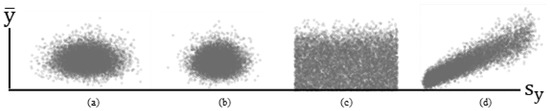
Figure 1.
Selected simulated (10,000 replications, n = 100) relationships between and s2. Left (a): iid normal RVs. Left middle (b): iid NB2 RVs. Right middle (c): i~id normal RVs. Right (d): i~id NBp RVs.
Theorem 1.
The linear correlation between and s2 for a mixture of independent and non-identically distributed (i~id) normal RVs is zero.
Proof of Theorem 1.
For a normal RV, μ can be any real value, and σ2 can be any positive real number. Because these two sets of values can be paired in any of the infinite number of possible ways that exist, each value of μ is paired with relatively large, intermediate, and small values of σ2, and each value of σ2 is paired with relatively large, intermediate, and small values of μ. Consequently, the linear correlation between these two variates is zero. □
This result (see Figure 1c; r = 0.001) is in contrast to that for an NBp RV for which μ appears in its variance formula, introducing linear correlation between the two (Figure 1d; r = 0.905). The formal postulation extension here is as follows:
Theorem 2.
The linear correlation between and s2 for a mixture of i~id NBp RVs is , p ≥ 1.
Proof of Theorem 2.
The linear product moment correlation coefficient is
because p > 0. □
- This new theorem indicates that if p = 1 (i.e., a Poisson RV), then ρ = 1, and for the standard NB2 case of p = 2, ρ ≈ 0.968. The parameter p needs to be 20 before this linear correlation is approximately 0.5. The dispersion parameter α does not affect this linear correlation. This new theorem indicates that for the aforementioned NBp, the sample mean and variance, and s2, are correlated (Figure 1d). In other words, the linear correlation between and s2 for a mixture of normal distributions is zero, whereas for a mixture of NBp distributions, it is asymptotically zero as p → ∞. Although this linear correlation remains zero when normal distributions are pooled, it can be as large as 1 for pooled NBp distributions.
Of note is that Theorem 1 holds even for a normal distribution restricted in such a way that σ2 = μ(1 + μp–1/α), with suitable restrictions on both p and μ (e.g., p must be even and the μ domain interval [–1, 0] must be removed from the range of σ2). Linear correlation occurs for this particular normal distribution case by, for example, imposing a constraint such as μ > 0, which then also allows p to be odd and linear correlation results to be described by Theorem 2.
3.2. MLE and Method of Moments Estimation (MME) of the Dispersion Parameter α
Various estimation techniques exist, including MLE, MME (e.g., see [6,13]), and least squares (see [14,15,16]). Frequently, these techniques yield exactly the same estimators. The estimation of the dispersion parameter 1/α of an NBp often is by MLE and/or MME. A μ closer to zero and a small sample size can create a situation in which an MLE and/or MME is inaccurate and/or unstable. MME is the simpler of the two techniques for estimating 1/α [5]. An MLE is unable to produce a solution that is an estimator in closed form for this NBp parameter (see Appendix A).
3.2.1. Estimation of Parameter Exponent p
Rather than setting p = 2, Equation (1) alludes to p as a parameter, albeit one restricted to the positive integers (i.e., discrete, not continuous). As a third parameter, its MME estimation requires, for example, adding the third moment about the mean, m3, to the set of estimation equations. Accordingly,
Solving this triplet of equations for p yields an equation that does not contain p, nor does the one incorporating the fourth moment. Thus, MME cannot render an estimate of p. Meanwhile, an MLE, which involves the difference calculus here because p is an integer, fails to produce a closed-form solution.
The implication of this outcome is that generalizing the standard NB2 variance term from μ(1 + μ/α) to the generalized NBp term μ(1 + μp–1/α) is similar to quasi-likelihood estimation with regard to parameter p. Denote with ; if seems too large, then a kth multiple of (i.e., ), where k is a positive integer, can be factored from it, effectively setting p = 2 + k. This factorization is nonconstant across the values of μi, with subscript i denoting an individual observation, when the mean varies from observation to observation (this is the situation Greene [1] presents).
3.2.2. A Simple n = 3 Numerical Example
Consider a sample of size n = 3, with the number of counts per observation, Y, being as follows: yi = {2, 5, 8}. Then
The MLEs are
The MMEs are
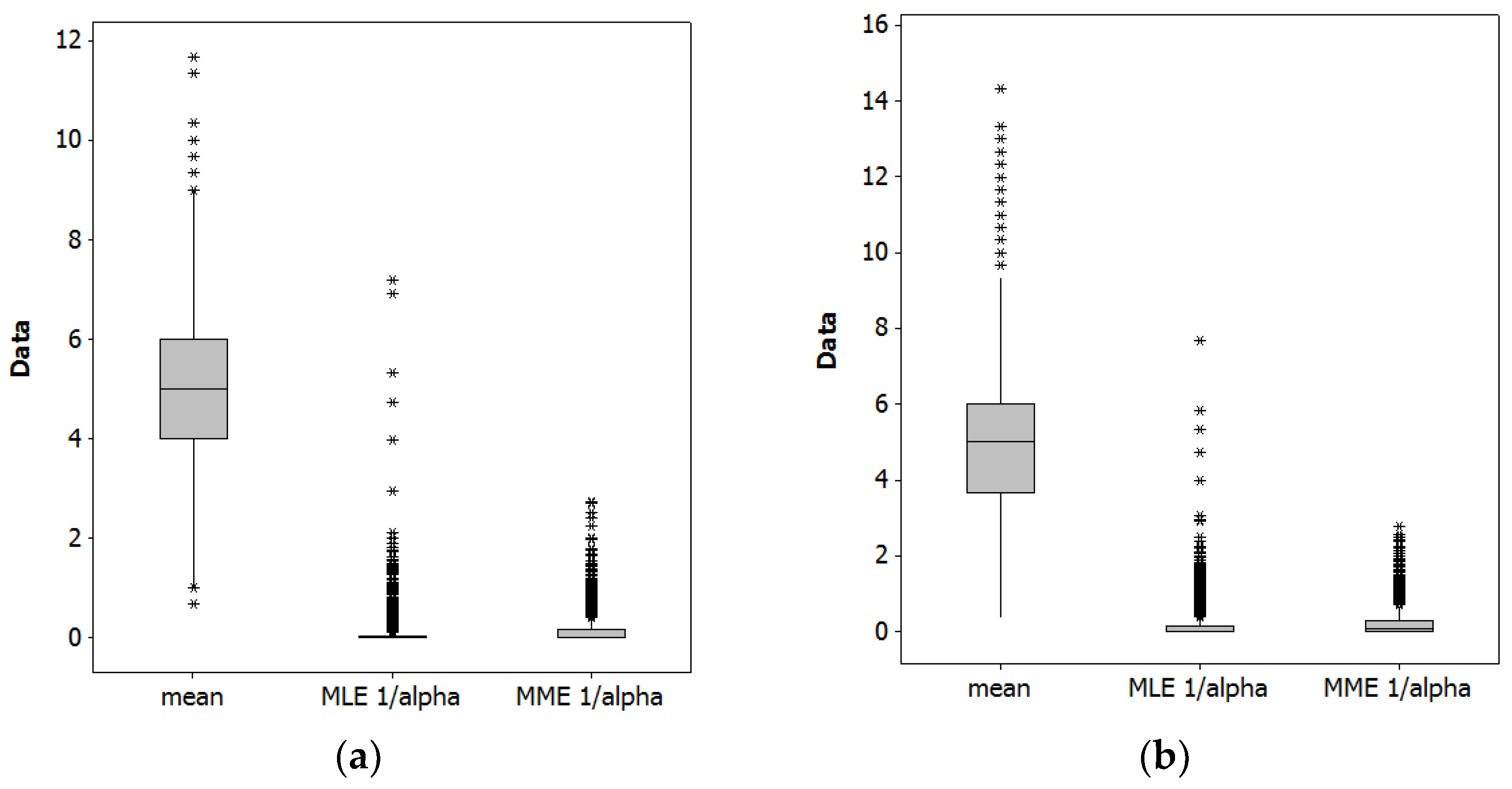
Table 1 summarizes results from a Monte Carlo simulation experiment with 10,000 replications (to invoke the Law of Large Numbers), for NB2[5, 5(1 + 5/0.0476)] and NB2[5, 5(1 + 5/0.1600)]. Figure 2 portrays the collective MLE and MME estimates for these simulation results.

Table 1.
Summary Monte Carlo simulation experiment results for NB2[5, 5(1 + 5/0.0476)] and NB2[5, 5(1 + 5/0.1600)].
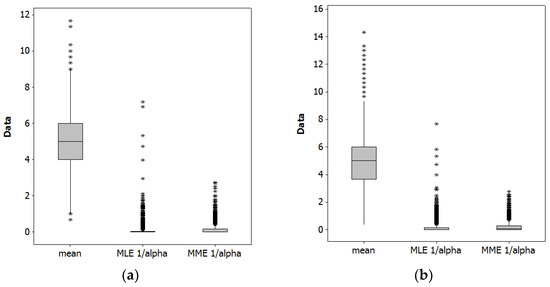
Figure 2.
Monte Carlo simulation experiment boxplots (as usual, asterisks denote outliers). Left (a): NB2[5, 5(1 + 5/0.0476)]. Right (b): NB2[5, 5(1 + 5/0.1600)].
As expected, both estimation techniques yield a sound estimate of the population mean, μ. The techniques furnish different estimates of the dispersion parameter, although both are within the 95% confidence interval of the other’s estimate. The MLEs are zero more often than MMEs are. Most of these zero MMEs actually are negative estimates that have been replaced by zero via truncation (these zero values were employed when calculating the summary statistics appearing in Table 1). These values should be considered infeasible because α is the shape parameter of a gamma RV, and as such must be positive. Figure 2 furnishes a visual box-and-whisker plot—the upper and lower edges of a box denote the first and third quartiles, the internal box line denotes the median, and the whisker tips denote 1.5 times the inter-quartile range (i.e., the third minus the first quartile values)—comparison between the two estimators (i.e., the MLEs and MMEs), highlighting that the MLEs have more outliers (denoted by asterisks). Excessive zeroes and frequency of outlier estimates for MLEs, and negative estimates for MMEs, are among the reasons these estimators are considered inaccurate and/or unstable. One general implication of these results is that neither estimator is particularly good for small samples, but that MME may well be preferable. This small sample case illustrates that an MLE and MME can yield different estimates (also see [17]).
3.2.3. Moran Eigenvector Spatial Filtering: A Brief Overview
The next section presents a simple example of interest, especially to criminologists, ecologists, entrepreneurs and marketers, environmental scientists, epidemiologists, geospatial analysts, sociologists, urban planners and urbanists, and urban and regional economists, among others, namely, population density, perhaps one of the most commonly utilized covariates in the social and behavioral sciences; it serves as a preface to Section 4. Georeferenced data require spatial statistics/econometrics methodology in order to properly account for latent SA in those data. SA is the correlation among observations that arises because of their relative proximity in geographic space, because either they are affected by some common factor or they directly interact with each other over geographic space. It is analogous to, but more complex than, serial correlation in time series data (e.g., see [18]).
Moran eigenvector spatial filtering (MESF) is a relatively novel methodology to handle SA contained in data [19,20,21]. MESF uses a set of synthetic proxy variables, which are extracted as eigenvectors from a doubly centered n-by-n spatial weights matrix (SWM), say C, that often is binary (0–1) and that ties n geographic objects together in space (indicating which are pairwise directly correlated by an entry of one), and then adds these vectors as control variables to a regression model specification; SWMs are analogous to undirected planar graph adjacency matrices. These control variables identify and isolate stochastic spatial dependencies among a set of georeferenced observations, filtering these dependencies out of a model’s residuals and adding them to the model’s mean response, thus allowing regression model building to proceed with georeferenced observations that mimic being independent.
The Moran Coefficient (MC; [22]) SA index, one of several such indices that exist—e.g., the Geary Ratio (GR; [23])—furnishes the basis for MESF; its numerator contains the doubly centered SWM exploited by MESF. This index can be written in matrix form as follows:
where n is the number of, for example, polygons in a geographic information system shapefile; Y is an n-by-1 vector of attribute values; I is an n-by-n identity matrix; 1 is an n-by-1 vector of ones; superscript T denotes matrix transpose and, here, C is a binary 0–1 SWM for which 1 denotes that the row and column areal units (i.e., locations, e.g., shapefile polygons) share a non-zero length common boundary, and 0 denotes that they do not (i.e., the rook adjacency definition, phraseology based upon chess game pieces and their moves). The eigenfunctions (i.e., the paired eigenvalues and eigenvectors) are extracted from the following matrix, which is doubly centered because matrix C is pre- and post-multiplied by the projection matrix (I − 11T/n), appearing in the numerator of expression (4) as follows:
When multiplied by (n/1TC1), an eigenvalue of matrix (5) is converted to the MC measuring the SA in its associated eigenvector map pattern of real number elements [24,25]. The sign of an eigenvalue indicates the nature of SA represented by its corresponding eigenvector, whereas its magnitude indicates the degree of SA. The extreme eigenvalues of matrix expression (4) determine the limits of MC, which are not necessarily ±1 [26].
(n/1T C1)YT(I − 11T/n)C(I − 11T/n)Y/YT(I − 11T/n)Y,
(I − 11T/n)C(I − 11T/n).
Extracting the eigenfunctions from adjusted SWMs constitutes a spectral decomposition of those matrices. The extracted eigenvectors with associated eigenvalues relatively far from zero, and hence representing other-than-negligible SA, may be viewed as portraying global, regional, or local components of SA because of the particular map patterns they depict when visualized [27,28]. In other words, SA manifests itself in terms of similar (positive SA; PSA) or dissimilar (negative SA; NSA) values of variable Y clustering on a map: hot spots (i.e., similar relatively high values clustering), cold spots (i.e., similar relatively low values clustering), or contrasts (i.e., relatively dissimilar values clustering).
3.2.4. An Empirical 2010 Puerto Rico Population Density Toy Illustration
Puerto Rico is partitioned into five agricultural administrative regions, as a scheme applied to it for a century or more, each focusing on one of the island’s major urban areas (Figure 3). The 1899 geographic distribution of population density for this spatial resolution displays excessive extra-Poisson variation (deviance = 1723, which is far greater than its expected value of 1) and moderate PSA. The table in Figure 3b reports the adjusted SWM eigenvector representing this PSA [MC = 0.221, with its maximum (MCmax) being 1.094, and GR = 0.474]. This scenario acknowledges a well-recognized source of over-dispersion, namely correlation among observations (i.e., dependent data, autocorrelation), which is frequent in spatial statistics; for example, SA accounts for roughly half of any detected over-dispersion (e.g., extra-Poisson variation).
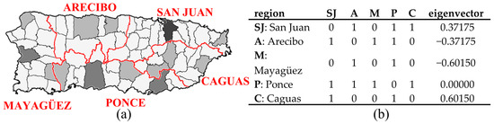
Figure 3.
The 1899 Puerto Rico agricultural administrative regions (AAR; denoted by red borders). Black lines denote municipio boundaries. Tertile choropleth map: black, gray, and white, respectively, denote relatively high, intermediate, and relatively low population density. Left (a): the municipality-AAR choropleth map. Right (b): the AAR spatial weights matrix and its relevant eigenvector.
An NB2 description of this geographic distribution of population density yields the global MLE of = e5.6361 ≈ 280.4 people per square mile, with a dispersion parameter MLE of ≈ 0.0010 (i.e., nearly a Poisson RV). The eigenvector spatial filter (ESF) specification, a linear combination of a subset of the eigenvectors extracted from the adjusted SWM, describes a spatially varying mean population density by region [i.e., 283.6 (SJ), 278.6 (A), 295.7 (M), 271.6 (P), and 272.4 (C)] about a global mean of 280.3 and reduces the over-dispersion parameter to 0.0006 (even more closely resembling a Poisson RV).
The global MME of also is e5.6361 ≈ 280.4. However, the dispersion parameter MME of is –0.0001, which would result in its being rounded to 0. Finally, the spatially varying mean population density by region is as follows: 280.1 (SJ), 280.6 (A), 280.8 (M), 280.4 (P), and 280.0 (C). These outcomes seem inferior to their preceding MLE counterparts.
4. Discussion: Two MESF Empirical Examples
The preceding examples in Section 3.2.2 and Section 3.2.4 are only for exemplification purposes. This section presents two empirical examples whose results furnish informative substantive implications.
4.1. An Empirical 2010 Puerto Rico Urban Population Density Case Study
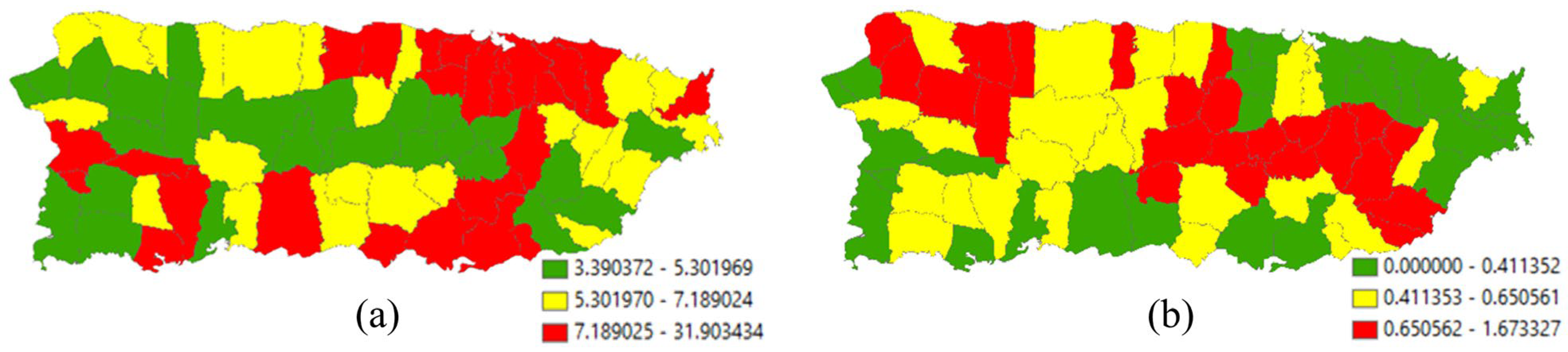
Figure 4a portrays the 2010 geographic distribution of urban population density (people per square mile) across the main island of Puerto Rico. The map pattern characterizing this geographic distribution has an MC of 0.487 and a GR of 0.541, implying moderate PSA. From the MLEs for an NB2 model specification, the global density is e7.0549 ≈ 1158.5, with a dispersion parameter of 0.6707 (i.e., sizeable extra-Poisson variation). Historically, the population has been concentrated on the coastal lowlands of the island, the preferred locations of the initial Spanish settlers because of convenience and accessibility, furnishing a rationale for including mean elevation as a covariate in an NB2 regression. Primarily because of the way urban areas expand (e.g., the establishment of infrastructure at the rural–urban fringe), this variable should contain PSA. In this case, executing NB2 stepwise regression estimation results in the selection of five PSA and no NSA eigenvectors from the candidate set extracted from the adjusted SWM for which MCj/MCmax ≥ 0.25, with subscript j denoting the jth eigenvalue. Table 2 summarizes the MLE results. It reveals that SA accounts for roughly 60% of the over-dispersion in these data, and the single covariate coupled with the constructed ESF accounts for more than three-fourths of the spatial variation in urban population density across the main island of Puerto Rico. With a final < 0.2, a dramatic shrinkage from nearly 0.7, p = 2 seems adequate for the NB model specification.

Figure 4.
Municipio geographic resolution 2010 population density (i.e., people per square mile) across the main island of Puerto Rico; green, yellow, and red, respectively, denote relatively low, intermediate, and high density values. Left (a): urban population (extra-Poisson variation is 41,183 >> 1). Right (b): rural population (extra-Poisson variation is 1427 >> 1).
Table 2.
Summary of model estimation results.
4.2. An Empirical 2010 Puerto Rico Rural Population Density Illustration
Figure 4b portrays the 2010 geographic distribution of rural population density across the main island of Puerto Rico. The map pattern characterizing this geographic distribution has an MC of 0.496 and a GR of 0.511, implying moderate PSA. From the MLEs for an NB2 model specification, the global density is e4.1298 ≈ 62.2, with a dispersion parameter of 1.8760. Rural and urban land are mutually exclusive, furnishing a rationale for including the density of rural land as a covariate. Because rural land tends to concentrate outside of urban areas, suggesting it contains PSA, and primarily because the expansion of urban land means the contraction of rural land, particularly along the rural–urban fringe, with this spatial competition suggesting it contains NSA, this variable should contain a PSA-NSA mixture. In this case, the stepwise NB2 estimation results in the selection of five eigenvectors, four with PSA and one with NSA (i.e., a mixture). Table 2 summarizes the MLE results. It reveals that SA accounts for roughly 26% of the over-dispersion in these data, and the single covariate coupled with the constructed ESF accounts for more than half of the spatial variation in rural population density across the main island of Puerto Rico. With a final > 1, p = 2 may seem inadequate for the NB model specification. Setting p = 3—with estimation executed via SAS PROC NLMIXED (see Appendix B), in which the NB3 probability density log-likelihood function was written expressing the modified NB as a general distribution [see https://stats.oarc.ucla.edu/sas/faq/how-can-i-compute-negative-binomial-models-with-random-intercepts-and-slopes-using-nlmixed/ (last accessed on 20 March 2024)], alters , which remains greater than one, while increasing the pseudo-R2 values when an ESF is present; these latter values decrease when p = 4, implying that p = 3 is the adequate value.
4.3. An Empirical 2010 Puerto Rico Rural Population Den
The two population density geographic distributions have markedly different island-wide averages and extra-Poisson variation. Although they have very similar SA index values, their ESFs indicate that they have very different latent map patterns (e.g., one is characterized by PSA, whereas the other is characterized by a mixture of PSA and NSA). A population classified as urban is not rural, and vice versa, which implies a negative relationship between these two geographic distributions. The bivariate Poisson RV correlation between them is –0.62 (see [33]). Finally, urban population density seems to be well described by an NB2 model, whereas rural population density may benefit from being described by an NB3 model.
5. Concluding Comments and Implications
This paper contributes to the academic literature in a number of different ways. First, it clarifies/corrects several inaccurate technical details in Greene’s earlier paper. Second, it presents new results that include the mgf for the NBp model, two new theorems, and original empirical spatial statistical/econometric applications. Third, it exemplifies selected small and large sample properties on NBp models. Finally, yet again, it demonstrates the power of MESF.
One prominent implication is that quantitative analysts, and especially applied spatial statisticians, studying Poisson and/or NB variables need to expand their toolbox to include NBp specifications for which p > 2. Another is the need for a wider appreciation and adoption of MESF-type methodology for correlated data, including for traditional dependent datasets, time series, and contemporary social network projects. A third repercussion of this paper is a recognition that the NBp random variable needs a Wikipedia page paralleling the existing one for the NB (https://en.wikipedia.org/wiki/Negative_binomial_distribution; last accessed on 15 May 2024).
Perhaps the most serious NBp limitation is its lack of closed-form MLEs. Although this variable drawback is not new to statistics, it does constitute an impediment to how the utilization of a variable flourishes. This certainly is a theme that should motivate subsequent research about the NBp. Another of its limitations is its newness, which means establishing strengths and weaknesses of employing it vis à vis alternative RVs is yet to be determined.
Funding
This research received no external funding.
Institutional Review Board Statement
Not applicable.
Informed Consent Statement
Not applicable.
Data Availability Statement
Data employed in this paper are readily available from the United States Census Bureau (i.e., the Puerto Rico data) or are obtainable (with sampling errors) by executing a suitable pseudo-random number generator (this paper used SAS implementations).
Acknowledgments
The author is an Ashbel Smith Chaired Professor of Geospatial Information Sciences.
Conflicts of Interest
The author declares no conflicts of interest.
Appendix A. Estimation of iid NBp Parameters
MLE
Both and produce the polygamma function (e.g., see [34]), involving the derivative of the logarithm of the gamma function, which prevents algebraically formulating closed-form solutions. In addition, the relationship among α, μ, and p determines whether or not an MLE exists.
MME (using the unbiased variance estimator)
Appendix B. SAS PROC NLMIXED Code
The following SAS code tricks its procedure into estimating a BN3 specification by not including a random effects term. The following input dataset (STEP3) contains the needed adjusted SWM eigenvectors, the response (i.e., population counts) and offset (i.e., log-area) variables, and the covariate (i.e., the logarithm of rural land area percentage; to avoid undefined terms for zero rural land, zero was replaced with one, which is trivial because the smallest non-zero measure is 9703):
PROC NLMIXED DATA = STEP3;
PARMS B0 = 0 B1 = 0 B2 = 0 B3 = 0 B4 = 0 B5 = 0 B6 = 0 A = 1.4;
P = 3;
*XB = B0 + OFFSET;
*XB = B0 + B1*PCTRL + OFFSET;
XB = B0 + B1*PCTRL + B2*COL10 + B3*COL12 + B4*COL15 + B5*COL20
+B6*COL44 + OFFSET;
MU = EXP(XB);
M = 1/A;
LL = LGAMMA(Y + M) − LGAMMA(Y + 1) - LGAMMA(M)
+Y*LOG(A*MU**(P - 1)) - (Y + M)*LOG(1 + A*MU**(P - 1));
MODEL Y ~ GENERAL(LL);
PREDICT MU OUT = MU;
RUN;
- XB differentiates between a constant mean, a bivariate regression with the rural area percentage covariate, and an MESF regression that includes this preceding covariate. P = 3 allows the estimation of NB3; setting P to 2 estimates NB2, and setting it to 1 estimates NB1 (i.e., a Poisson). Finally, the temporary SAS file WORK.MU stores predicted counts for post-processing. The NB1 and NB2 options support comparative output checks with other software modules.
References
- Cameron, C.; Trivedi, P. Regression Analysis of Count Data; Cambridge University Press: New York, NY, USA, 1998. [Google Scholar]
- Barreto-Souza, W.; Ombao, H. The negative binomial process: A tractable model with composite likelihood-based inference. Scand. J. Stat. 2021, 49, 568–592. [Google Scholar] [CrossRef]
- Greene, W. Functional forms for the negative binomial model for count data. Econ. Lett. 2008, 99, 585–590. [Google Scholar] [CrossRef]
- Di, Y.; Schafer, D.W.; Cumbie, J.S.; Chang, J.H. The NBP Negative Binomial Model for Assessing Differential Gene Expression from RNA-Seq. Stat. Appl. Genet. Mol. Biol. 2011, 10, 1–28. [Google Scholar] [CrossRef]
- Zhang, Y.; Ye, Z.; Lord, D. Estimating dispersion parameter of negative binomial distribution for analysis of crash data: Bootstrapped maximum likelihood method. Transp. Res. Rec. J. Transp. Res. Board 2019, 2019, 15–21. [Google Scholar] [CrossRef]
- Pearson, K. Method of Moments and Method of Maximum Likelihood. Biometrika 1936, 28, 34–59. [Google Scholar] [CrossRef]
- Hendry, D.; Nielsen, B. Econometric Modeling: A Likelihood Approach; Princeton University Press: Princeton, NJ, USA, 2007. [Google Scholar]
- Chambers, R.L.; Steel, D.G.; Wang, S.; Welsh, A. Maximum Likelihood Estimation for Sample Surveys; CRC Press: Boca Raton, FL, USA, 2012. [Google Scholar]
- Rossi, R. Mathematical Statistics: An Introduction to Likelihood Based Inference; Wiley: New York, NY, USA, 2018. [Google Scholar]
- Ward, M.; Ahlquist, J. Maximum Likelihood for Social Science: Strategies for Analysis; Cambridge University Press: New York, NY, USA, 2018. [Google Scholar]
- Hoeffding, W. The Large-Sample Power of Tests Based on Permutations of Observations. Ann. Math. Stat. 1952, 23, 169–192. [Google Scholar] [CrossRef]
- Bagui, S.; Mehra, K. On the convergence of negative binomial distribution. Am. J. Math. Stat. 2019, 9, 44–50. [Google Scholar]
- Bowman, K.; Shenton, L. Estimator: Method of moments, Encyclopedia of Statistical Sciences, vol. 3 (D’Agostino Test of Normality to Eye Estimate), 2nd ed.; Kotz, S., Read, C., Balakrishnan, N., Vidakovic, B., Johnson, N., Eds.; Wiley: New York, NY, USA, 2006; pp. 2092–2098. [Google Scholar]
- van de Geer, S. A New Approach to Least-Squares Estimation, with Applications. Ann. Stat. 1987, 15, 587–602. [Google Scholar] [CrossRef]
- van de Geer, S. Least squares estimation. In Encyclopedia of Statistics in Behavioral Science; Everitt, B., Howell, D., Eds.; Wiley: Chichester, UK, 2005; Volume 2, pp. 1041–1045. Available online: https://people.math.ethz.ch/~geer/bsa199_o.pdf (accessed on 1 March 2024).
- Wolberg, J. Data Analysis Using the Method of Least Squares: Extracting the Most Information from Experiments; Springer: Berlin, Germany, 2005. [Google Scholar]
- Delicado, P.; Goria, M.N. A small sample comparison of maximum likelihood, moments and L-moments methods for the asymmetric exponential power distribution. Comput. Stat. Data Anal. 2008, 52, 1661–1673. [Google Scholar] [CrossRef]
- Griffith, D.A. A Family of Correlated Observations: From Independent to Strongly Interrelated Ones. Stats 2020, 3, 166–184. [Google Scholar] [CrossRef]
- Griffith, D. Spatial filtering. In Encyclopedia of Geographic Information Science; Kemp, K., Ed.; SAGE: Thousand Oaks, CA, USA, 2008; pp. 413–415. [Google Scholar]
- Griffith, D.; Getis, A. Spatial filtering. In Encyclopedia of GIS, 2nd ed.; Shekhar, S., Xiong, H., Zhou, X., Eds.; Springer: Cham, Switzerland, 2016; pp. 1–14. [Google Scholar] [CrossRef]
- Griffith, D.; Chun, Y. Spatial Autocorrelation and Spatial Filtering. In Handbook of Regional Science, 2nd ed.; Fischer, M., Nijkamp, P., Eds.; Springer-Verlag: Berlin, Germany, 2022; pp. 1863–1892, (revised, update to 2014 version). [Google Scholar]
- Moran, P. The interpretation of statistical maps. J. R. Stat. Soc. B 1948, 10, 243–251. [Google Scholar] [CrossRef]
- Geary, R.C. The Contiguity Ratio and Statistical Mapping. Incorp. Stat. 1954, 5, 115–127+129–146. [Google Scholar] [CrossRef]
- Tiefelsdorf, M.; Boots, B. The exact distribution of Moran’s I. Environ. Plan. A 1995, 27, 985–999. [Google Scholar] [CrossRef]
- Griffith, D.A. Spatial autocorrelation and eigenfunctions of the geographic weights matrix accompanying geo-referenced data. Can. Geogr. Can. 1996, 40, 351–367. [Google Scholar] [CrossRef]
- de Jong, P.; Sprenger, C.; van Veen, F. On extreme values of Moran’s I and Geary’s c. Geogr. Anal. 1984, 16, 17–24. [Google Scholar] [CrossRef]
- Borcard, D.; Legendre, P. All-scale spatial analysis of ecological data by means of principal coordinates of neighbour matrices. Ecol. Model. 2002, 153, 51–68. [Google Scholar] [CrossRef]
- Borcard, D.; Legendre, P.; Avois-Jacquet, C.; Tuomisto, H. Dissecting the spatial structure of ecological data at multiple scales. Ecology 2004, 85, 1826–1832. [Google Scholar] [CrossRef]
- Cameron, A.C.; Windmeijer, F.A.G. An R-squared measure of goodness of fit for some common nonlinear regression models. J. Econ. 1997, 77, 329–342. [Google Scholar] [CrossRef]
- Christensen, R. General Prediction Theory and the Role of R2, Unpublished Manuscript; Department of Mathematics and Statistics, University of New Mexico: Albuquerque, NM, USA, 2007; Available online: https://www.math.unm.edu/~fletcher/JPG/rsq.pdf (accessed on 1 March 2024).
- Hoetker, G. The use of logit and probit models in strategic management research: Critical issues. Strat. Manag. J. 2007, 28, 331–343. [Google Scholar] [CrossRef]
- Cakmakyapan, S.; Demirhan, H. A Monte Carlo-based pseudo-coefficient of determination for generalized linear models with binary outcome. J. Appl. Stat. 2016, 44, 2458–2482. [Google Scholar] [CrossRef]
- Kawamura, K. The structure of bivariate Poisson distribution. Kodai Math. J. 1973, 25, 246–256. [Google Scholar] [CrossRef]
- Mortici, C. Very accurate estimates of the polygamma functions. Asymptot. Anal. 2010, 68, 125–134. [Google Scholar] [CrossRef]


Disclaimer/Publisher’s Note: The statements, opinions and data contained in all publications are solely those of the individual author(s) and contributor(s) and not of MDPI and/or the editor(s). MDPI and/or the editor(s) disclaim responsibility for any injury to people or property resulting from any ideas, methods, instructions or products referred to in the content. |
© 2024 by the author. Licensee MDPI, Basel, Switzerland. This article is an open access article distributed under the terms and conditions of the Creative Commons Attribution (CC BY) license (https://creativecommons.org/licenses/by/4.0/).