Abstract
At every point on a smooth -manifold M there exist skew-symmetric tensor spaces spanning differential -forms with . Because is always zero where is the exterior differential, it follows that every exact -form (i.e., where is an -form) is closed (i.e., ) but not every closed -form is exact. This implies the existence of a third type of differential -form that is closed but not exact. Such forms are called harmonic forms. Every smooth -manifold has an underlying topological structure. Many different possible topological structures exist. What distinguishes one topological structure from another is the number of holes of various dimensions it possesses. De Rham’s theory of differential forms relates the presence of -dimensional holes in the underlying topology of a smooth -manifold to the presence of harmonic -form fields on the smooth manifold. A large amount of theory is required to understand de Rham’s theorem. In this paper we summarize the differential geometry that links holes in the underlying topology of a smooth manifold with harmonic fields on the manifold. We explore the application of de Rham’s theory to (i) visual, (ii) mechanical, (iii) electrical and (iv) fluid flow systems. In particular, we consider harmonic flow fields in the intracellular aqueous solution of biological cells and we propose, on mathematical grounds, a possible role of harmonic flow fields in the folding of protein polypeptide chains.
Keywords:
simplicial complexes; singular homology groups; singular cohomology groups; singular chain complexes; Grassmann algebra; Laplacian and harmonic forms; de Rham cohomology groups; de Rham’s theorem; protein folding MSC:
53Z10; 53Z30
1. Introduction
A well-known quote of Einstein says that as far as the laws of mathematics refer to reality, they are not certain, and as far as they are certain, they do not refer to reality. While this may be seen as controversial, it certainly is the case that mathematical theories of physical processes require interpretation in terms of experimental observations. Differential geometry is a logical structure of provable propositions, theorems and lemmas whose truth derives from axioms, definitions and the elementary connectives of formal logic. To apply differential geometry to physical systems requires the construction of bridges between events and variables in the physical world (preferably, but not necessarily, measurable) and well-defined notions in the deductively logical structure of differential geometry. These bridges are intuitive hypotheses linking reality to mathematics and their value derives from the quality of the intuition of the practitioner. If the hypothesis is true, then certain laws of mathematics can be applied to the real-world system. But even if it is demonstrated experimentally that the mathematical laws do describe the real-world behavior, this does not prove the hypothesis. Other hypotheses may do equally well. Indeed, it is not possible to prove if-then conjectures, although they can be easily proven false. In applied mathematics, the ‘if-then bridges’ between reality and mathematics remain forever intuitive. With respect to certainty, it is the mathematics that is primary.
That said and understood, there is value in showing that the same mathematics can apply usefully to a range of real-world systems.
De Rham’s cohomology theorem of differential forms is a remarkable piece of mathematics that links together areas of mathematics that were previously thought unrelated. We believe that the mathematical facts provided by de Rham’s theorem have great relevance to the nonlinear behavior and the presence of critical points and singularities in the state spaces of many different real-world systems. In this paper, we consider an interpretation of the theorem in terms of experimental observations of the dynamics of fluid flow. In essence, de Rham’s cohomology theory relates the existence of holes of various dimensions in the underlying topology of smooth and Riemannian manifolds with a third type of differential form flow field on the manifold, one that is closed but not exact. Such a flow field is called an harmonic field. In other words, our aim is to demonstrate the links between the harmonic fields of mathematics and physical flows of real-world nonlinear systems with singularities and critical points observed in nature.
To illustrate the sort of nonlinear dynamical processes in the world that can be understood through this mathematical linking, consider the bubbles and fluid flow associated with pouring a glass of champagne, or the generation and flow of foam associated with an ocean wave breaking on a beach, or the chaotic turbulent flow of a mountain stream around rocks. Even the metamorphosis of a caterpillar into a moth may be within the scope of the theory. Certain singularities in the nonlinear dynamics of visual, mechanical, electrical, and fluid-flow systems can be related to harmonic fields. In particular, we will examine the possible role of vortices and eddies in harmonic flow fields induced by the presence of organelles and other molecules immersed in the intracellular aqueous solution of biological cells on the kinetics of protein folding.
Our search for this linking was inspired by two seemingly unrelated happenings. Firstly, in our analysis of the geometry of 3D binocular visual space [1,2,3], we came to realize that three different 3D geometries have to be taken into account. There is of course the 3D Euclidean geometry of the outside world. But the geometry of the 3D visual space encoded by sensory receptors is warped (or curved) by the fact that the size of images on the retinas of the eyes vary in inverse proportion to the Euclidean distance between the object in the environment and the nodal point of the eye [4]. This intrinsic 3D space corresponds to a curved Riemannian manifold with a metric proportional to the inverse of the Euclidean distance squared [1]. This gives rise to a singularity at the origin where the metric goes to infinity. The consciously perceived 3D visual space is different again because many different cognitive mechanisms of depth perception are brought into play. The singularity at the origin is taken care of by the existence of a hole about the egocenter in visual space. Existence of such a hole is confirmed by the fact that it is not possible to see your own head, let alone your own egocenter. This raises the question, what effect does such a hole in visual space have on the perceived flow of visual images?
The second event concerned an unusual cluster of breast cancer diagnoses that occurred in women working together at an Australian television studio [5,6]. It was speculated that the cancers might be caused by leakage of electromagnetic radiation from the TV transmitter. Experts were brought in to test this hypothesis. They found no evidence of any problematic radiation levels in the women’s workplace. In physical theories of electromagnetism, there are at least two types of electric field. One is given by voltage gradients and the curl of the other is given by changing magnetic fields. These two types of field are independent because the curl of a gradient is always zero. The question arises, is there a mysterious third type of electric field that would have gone undetected by the standard measurement techniques? Differential geometry suggests that there is. According to de Rham’s theorem, the curl of an electric field can be zero without it being the gradient of a voltage. The question becomes, does such a third type of field exist in nature and if so, what properties does it have?
Applying differential geometry to physical systems requires a thorough knowledge of the mathematical theory, because the sequence in which it is applied does not necessarily follow the beautiful logical sequence in which the theorems were developed and proven. Application often requires jumping from one point in the mathematical theory to a distant point with a large amount of mathematics linking the two points. Moreover, an understanding of de Rham’s theorem is not trivial. It requires familiarity with a large amount of differential geometry. Consequently, in Appendix A we provide detail of all the steps in our proposed mathematical linking between the appearance and disappearance of holes in the underlying topology of smooth and Riemannian manifolds and the appearance and disappearance of harmonic flow fields on the manifold. Meanwhile, in the following section we provide the reader with a more conceptual introduction to the differential geometry used in relating topological bifurcations to chaotic flow fields in nature.
2. A Summary of Relevant Differential Geometry Concepts
2.1. Topological Structure
An important property of topological spaces is that they are not equipped with a metric. They have no measure of size. Size and topology can be thought of as independent properties. A topological space, like the set of all points on a 2-sphere, can be expanded to the size of a planet or contracted to the size of an atom without changing its topological structure. So long as it is not cut, torn, punctured or any parts of it glued together, it can be deformed in any way by any amount without changing its topological structure. For example, the 2-sphere can be stretched into a long thin rope and tied into a knot without changing its topology.
All the different shapes a topological space can be deformed into without cutting, tearing, puncturing or gluing can be mapped in a continuous, one-to-one, onto and continuously invertible fashion to each other. This is a special type of map called a homeomorphism. Any two homeomorphic spaces have all the same topological properties. Indeed, a topological property can be defined as one that is preserved by homeomorphic maps. Transformations that leave the topological structure unchanged are called homotopies, a well-known example being the transformation of a coffee mug with a handle into a donut and vice versa [7]. The mathematical mapping ([8], p. 348) is shown in Figure 1.
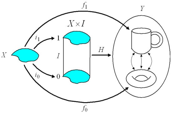
Figure 1.
A diagram illustrating homotopy. The 2-torus (surface of a donut) in the topological space and the coffee mug with handle in the topological space are equivalent topological structures. These are not only homeomorphically related (i.e., continuous, one-to-one, onto and invertible) but there are continuous homotopic maps that map the topological space to both the 2-torus and the mug. The fact that the donut can be continuously transformed into the mug implies the existence of all the intermediate shapes in the transformation. The hole in the donut morphs into the hole between the mug and its handle. This is illustrated in the diagram by the special case in which , , , where the interval varies from to . For each point , the map corresponds to the 2-torus, the map corresponds to the mug and all the other points along the interval correspond to the intermediate shapes. This is represented in the diagram by the homotopy . More generally, while the topological spaces and can include holes of various dimensions, they must have the same topological structure in order for the homotopy to exist. In other words, for to be homotopic maps, the induced homomorphisms for all between the homology groups for and must be equal, i.e.,
There is no way, however, that a 2-sphere can be transformed into a 2-torus without puncturing holes into the sphere. The 2-sphere and the 2-torus do not have the same topological structure. It was shown by A.A. Markov in 1958 (see [8]) that there is no algorithm that can determine all the different topological structures a topological space with dimension 4 or greater can have. The best we can say is that such spaces have a large number of possible different topological structures. Basically, what makes topological structures different is the different number of holes of various dimensions that exist in the topological space (e.g., the difference between the topology of a sphere and the topology of a torus is attributable to the hole(s) in the torus).
2.2. Topological Bifurcations
Based on Smale [9], Abrahams and Marsden [10] provide a description of bifurcations in the underlying topology of a smooth manifold. A smooth map between smooth manifolds and is locally trivial at if there is a neighborhood of such that is a smooth properly embedded submanifold (i.e., a level set) in for each in and there are diffeomorphic maps for each (i.e., projects nearby level sets in diffeomorphically onto the level set .
The bifurcation set of is In other words, as passes through , changes its topological structure. Let denote the closed set of critical points of in , i.e.,
By Sard’s theorem, the singular values in have measure zero (i.e., they are isolated points with empty interior and their union is nowhere dense in ). The singular values of are the bifurcation values of in [10]. In other words, the level sets in of singular bifurcation values in have a topological structure that differs from the topological structures of neighboring level sets in . The number of holes in the level set in of a bifurcation value in differs from the number of holes in the neighboring level sets. This can be related to isotropy subgroups, the slice theorem, the tube theorem, the -orbit type submanifold, the -isotropy type submanifold and the -fixed point type submanifold described by Ortega and Ratiu [11] that extend the notion of critical points in submanifolds.
2.3. De Rham’s Theory
We provide here only a brief description. A more expanded summary of differential geometry linking bifurcations with harmonic flow fields is given in Appendix A.
Every exact differential -form with on a smooth -dimensional manifold or an -dimensional Riemannian manifold is closed (i.e., ) because is always zero. But a closed differential -form is not necessarily exact. Differential -forms that are closed but not exact give rise to a third type of differential -form. There are thus three types of differential -forms, (i) -forms whose exterior derivative is not zero (i.e., ), (ii) closed -forms that are exact differentials (i.e., where is an -form) and (iii) -forms that are closed but not exact. This third type of -form is called an harmonic -form and is contained in the -th harmonic space of the manifold with . It is also an element in the -th de Rham cohomology group with . is isomorphic with . Both and are vector subspaces as well as being groups.
If is a closed -form (i.e., ) on a smooth manifold , and is an -dimensional cycle in the underlying topology of the manifold, then the integral of over is called a period of (the term period derives from the periods of elliptic integrals). From Stokes’ theorem, if the -cycle happens to be a boundary of an -chain (i.e., ), then the period vanishes since
(See Appendix A.1 for definitions of chains, cycles and boundaries).
From this we obtain de Rham’s first theorem: a closed form is globally exact if and only if all of its periods vanish [12]. Knowing which forms are globally exact and which are not has important consequences. For example, (i) a smooth 1-form is conservative (i.e., its line integral is path-independent) if and only if it is exact, (ii) the integral of every globally exact form over a compact oriented smooth manifold without boundary is zero, (iii) the integral of globally closed forms over boundaries is zero and (iv) if the integral of a closed -form over an -dimensional submanifold without boundary is not zero, then the -form is not exact and the submanifold is not the boundary of a compact oriented submanifold with boundary.
A remarkable property of harmonic spaces and de Rham cohomology groups is that they are homotopically and topologically invariant. They are isomorphic to singular cohomology groups , and these in turn are isomorphic to singular homology groups on the underlying topological structure of the smooth manifold (see Appendix A.12). This is depicted in Figure 2.

Figure 2.
A diagram illustrating the fact that if are diffeomorphic maps between smooth manifolds and , then the pull-back maps between the de Rham cohomology groups and for all values of are equal, i.e., . In other words, if the maps and are diffeomorphic, they have the same homeomorphic topological structure and so they are homotopy-invariant. This means that homotopy-equivalent manifolds have isomorphic de Rham groups. The labels represent the skew-symmetric tensor spaces of degree and degree for differential forms at each point on the smooth manifold . The labels represent the skew-symmetric tensor spaces of degree , degree and degree for differential forms at each point on the smooth manifold . The maps for all values of are called homotopy operators. Examination of the diagram shows that if the -form is closed, i.e., , then . In other words, and differ by an exact differential . The maps are said to be cohomologous. This is exactly how equal cohomology groups are defined. Therefore, cohomologous groups have isomorphic de Rham cohomology groups.
This is indeed a remarkable property, because it is not immediately obvious that closeness and exactness of differential forms on a smooth manifold should have anything to do with the underlying topological structure of the manifold. But de Rham’s theory shows mathematically that they do! The -th homology group is isomorphic to the -th de Rham cohomology group with . detects the presence of -dimensional holes in the underlying topology of the smooth manifold . The dimension of equals the number of -dimensional holes in the topology, and this is known as the -th Betti number of the manifold. Thus, de Rham’s theory of differential forms provides the link we are looking for between holes in the topological structure of a smooth or Riemannian manifold and harmonic flow fields on the manifold.
2.4. The Hodge Laplacian Operator
By definition, the Hodge Laplacian operator on a Riemannian manifold is , where is the exterior derivative , , where is the Hodge star operator and is the skew-symmetric tensor space of -forms for at every point on an -dimensional smooth manifold or a Riemannian manifold . The Laplacian operator plays an important role in de Rham’s theory of differential forms because it is the only operator that can be used to compute harmonic forms on a Riemannian manifold. The harmonic space for . (Keep in mind that harmonic -forms for all values of on a smooth manifold or a Riemannian manifold are associated with the presence of -dimensional holes in the underlying topology of the manifold).
2.5. Harmonic 0-Forms and 1-Forms
Harmonic 0-forms are given by the equation , where is a smooth real-valued function on the smooth manifold or Riemannian manifold . Potential fields in a fluid are irrotational and incompressible (i.e., divergence-free) harmonic 0-forms. We focus here on computing harmonic 1-forms on Riemannian manifolds because of their importance in the nonlinear dynamics of the physical systems to be discussed below. Let be a differential 1-form in at each point . First, we compute the Hodge Laplacian of a 1-form on a Riemannian manifold , i.e., , and then we compute the harmonic 1-form by setting the Laplacian .
The Ricci curvature tensor can be described geometrically as follows. Let be a Riemannian manifold and a point belonging to (i.e., ). For every unit vector , is the sum of the sectional curvatures of the 2-planes in spanned by , where is any -orthonormal basis for with . Given any unit vector , choose a -orthonormal basis for such that . Then is given by
Following Lang [13] (pp. 423–424), the inner product of the Ricci curvature tensor with the vector (i.e., ) is defined to be the scalar-valued form such that, with respect to an orthonormal frame , and any unit vector field with , we have
where we denote by the value of the 1-form on the vector field . As an operator on 1-forms, the Laplacian is given by . Written in terms of variables, this means .
To compute the Hodge Laplacian inner product , we compute (i) and (ii) separately and then add:
- (i)
- We have , where is the dual of the 1-form field and for is a -orthonormal frame of vector fields. These orthonormal vectors have to be computed using the Riemannian metric Gram–Schmidt orthogonalizing algorithm at each point. We see that is a real-valued function on . For each point , we have . Thus we can write
- (ii)
- To obtain , we first note that if is an -form, we can use the propositionwhere is a 1-form and and are vectors. Using the fact that for any -formwhere for is an orthonormal frame and for is an orthonormal coframe, it follows thatwhere is notation for contracted by [13].From Equations (3) and (2) with , we obtain [13] (p. 424)
Finally, we add Equations (1) and (4) to obtain
Thus, for a 1-form on an -dimensional Riemannian manifold , the Hodge Laplacian operator has the form , where is the Ricci curvature operator. The harmonic 1-form is then obtained by setting the Laplacian equal to zero.
3. Physical Examples
There exists an endless variety of behaviors in nature of nonlinear dynamical systems associated with different singularities, critical points and degeneracies in their differential equations. Most of these behaviors have not yet been described, let alone solved. One family of such behaviors considered in this paper is associated with the existence of holes of various dimensions in the underlying topology of the state space of the system. Such holes create differential forms and vector fields that are closed but not exact and create ‘no-go’ spaces in the dynamical state of the system. Such holes can dramatically change the dynamical behavior of the system. Isotropy subgroups in the action of a Lie group on a dynamical system, for example, create dynamic states that a vector field (or subset of vector fields) can flow into but not out of; a type of equilibrium point dynamical-state trap. But nonlinear dynamical systems can transition to neighboring vector fields and flow around the trap, creating novel nonlinear behaviors [11]. In what follows, we consider the consequences on dynamical behavior of singularities in the differential equations that give rise to differential forms that are closed but not exact in visual, mechanical, electrical and fluid-flow physical systems.
3.1. The Human Visual System
Human binocular 3D visual space encoded by visual, proprioceptive and vestibular sensory receptors is warped (or curved) because the size of 2D images on the retina of each eye varies in inverse proportion to the Euclidean distance between the nodal point of the eye and the object in the environment. Geometrically speaking, 3D visual space corresponds to an egocentric negatively curved Riemannian manifold with a 3D ball of points missing from about the origin (i.e., egocenter) [1,2]. This intrinsic hole corresponds to the fact that it is not possible to see your own head. What influence does such a hole about the origin in 3D warped visual space have on the perceived flow of visual images? Differential geometry and de Rham’s theorem provide a possible answer to this question. (Note that other holes in 3D visual space are possible due to neural pathology. Known as scotomas, these are not considered here.)
Given a 2D hole about the origin (i.e., a missing 3D ball of points about the origin enclosed within a 2-cycle), de Rham’s theorem implies that closed differential -forms for are not globally exact. The unit volume form is a closed 3-form on the warped 3D visual space, and therefore the hole about the origin prevents this volume 3-form from being globally exact. This is just as well, because if there was no hole about the origin and the closed volume form was globally exact, then all the periods equal to the volume form integrated over all 3-chains (i.e., volumes) enclosed by 2-cycles would vanish. The underlying topology of the warped 3D visual space would be such that the perceived volume of any enclosed 3D space would equal zero. In other words, it would not be possible to sense the size (i.e., volume) of enclosed 3D spaces. We know from everyday experience that we can visually sense the size of the room we are in. This is as predicted by de Rham’s theorem.
3.2. Mechanical Systems
In the absence of all external forces, Hamiltonian mechanics plays out on the -dimensional cotangent bundle (or momentum phase space) of an -dimensional configuration manifold . Using position (configuration) and momentum as canonical coordinates, a canonical 1-form and a canonical closed 2-form exist at every point on (i.e., on the momentum phase space of the Hamiltonian system). The symplectic structure of the 2-form defines a symplectic geometry on the system. Contraction of the symplectic 2-form field by a vector field gives a 1-form field on . However, there is a wonderful discovery that applies to all Hamiltonian mechanical systems (and to all systems whose dynamics can be described by 2nd-order differential equations). There exists a special vector field for which the 1-form field is an exact 1-form field equal to , where is a smooth real-valued function on the momentum phase space . The real-valued function is called the Hamiltonian function, and the vector field is called the Hamiltonian vector field of the Hamiltonian mechanical system. If the real-valued function is equal to the total energy of the mechanical system (i.e., equal to the sum of the kinetic energy and potential energy of the system expressed as a function of position and momentum), then the integral flow of the Hamiltonian vector field in the momentum phase space is equal to the free motion of the mechanical system. Since by definition there is no energy-injecting or energy-dissipating external force, the integral flow of the Hamiltonian vector field conserves the total energy of the system. The integral flow is confined to a -dimensional constant energy (i.e., constant ) contour shell in . Different energy levels correspond to flows in different constant energy contour shells in the momentum phase space of the system.
However, if there exists a 1-dimensional hole in the momentum phase space, then, from de Rham’s theorem, the 1-form cannot be globally exact, and hence neither the Hamiltonian function nor the Hamiltonian vector field can be globally defined! The exact 1-form field is replaced by an harmonic 1-form field
that is closed but not exact.
3.3. Electrodynamical Systems
In electrodynamics on Minkowski 4D spacetime, Maxwell’s equations can be written in terms of differential forms as
where is a skew-symmetric electromagnetic 2-form at each point in 4D Minkowski spacetime, is a current 4-vector at each point, is the speed of light in a vacuum and is the Hodge star operator (all in Gaussian units).
The source-free equations are true if and only if there exists a 4-covector field (i.e., a 1-form field) called the electromagnetic potential field such that (i.e., is a closed, globally exact 2-form field on 4D flat Minkowski spacetime).
Such a 1-form field can be altered by the addition of an exterior differential of a smooth real-valued function on the 4D Minkowski manifold (i.e., =) without changing the closed 2-form electromagnetic field . is unchanged because is always zero, and can be written as
Any such transformation of the electromagnetic potential that has no effect on the electromagnetic field is called a gauge transformation. Any choice of that satisfies the inhomogeneous wave equation is called a Lorentz gauge; i.e.,
where the operator is the wave operator or the d’Alembertian
This shows that an electromagnetic potential in the Lorentz gauge can carry an electromagnetic wave propagating at the speed of light in a vacuum without changing the electromagnetic field . The electromagnetic field is the medium in which the wave propagates with no need of an aether. It is important to notice that
i.e., the d’Alembertian wave operator on 4D flat Minkowski spacetime is equal to the Laplacian on a flat 4D spacetime.
However, if a 1-dimensional hole exists in the 4D spacetime manifold, then, from de Rham’s theorem, the electromagnetic potential cannot be globally exact, and consequently the Lorentz gauge cannot be defined. The global electromagnetic potential 1-form field is replaced by an harmonic 1-form field. This leaves the question about the existence of an aether uncertain.
3.4. Fluid Flow
The principles of fluid mechanics have long been a standard in the teaching of physics [14,15,16]. Consider a slowly flowing stream of water. Water particles close to the boundary adhere to the boundary and so have zero downstream velocity. Water molecules in this boundary layer form hydrogen bonds with each other that increase surface tension and alter the dipole distribution of electric charge. Points away from the boundary towards the center of the stream have higher average downstream flow velocities. This pattern of flow is known as lamina flow. The random motion of water particles due to thermal energy and electric fields causes an interchange of water particles between the various laminae, with the higher-velocity particles speeding up the slower ones and vice versa. This gives rise to shear stresses and transfer of kinetic energy and momentum between the various layers producing a property of the water known as its dynamic viscosity . Viscosity varies between different fluids and provides a measure of the ease of flow. Honey, for example, has a higher viscosity than water and flows less easily.
Now consider a fast-flowing mountain stream flowing around rocks. Water particles cannot flow through the rocks, so they have to flow around them. The rocks form 2D holes of various sizes in the space of the water (i.e., the 2D surface of each rock is a 2-cycle that forms a boundary about a hole in the space of water flow). If the stream is flowing fast enough (due to an ample supply of kinetic energy provided by gravity), flow around the rocks induces large eddies and vortices in the flow. These large eddies propagate outwards, transferring kinetic energy to smaller eddies and vortices. These in turn generate even smaller eddies. This cascade of kinetic energy from larger to smaller eddies depends on the velocity of flow (i.e., available kinetic energy) and the rate of energy dissipation in the water due to viscosity. The eddies of various sizes appear and disappear in an unpredictable fashion, causing local tangential velocities and pressures to vary from point to point in a chaotic unpredictable fashion. This increases the amount of mixing. Increased local flow velocities reduce local pressure, allowing gases in the water to vaporize and produce bubbles. Formation and popping of bubbles dissipate energy and produce a ‘gurgling’ sound. The chaotic pattern of flow associated with such a cascade of energy from large to small eddies with minimal energy dissipation is called turbulent flow. Turbulent flow is observed in many fluid flows in nature, such as ocean waves, storm clouds, smoke, bubbles in champagne and more.
3.4.1. Navier–Stokes Equations
The Navier–Stokes equations are nonlinear partial differential equations that describe the motion of viscous fluids in 3D Euclidean space. They were developed over many years during the first half of the 1800s by Navier and Stokes. In essence, they are an expression of Newton’s second law of motion; that is, force equals mass times acceleration. The incompressible Navier–Stokes equations can be derived from the convective form of the Cauchy momentum equation and have the form
Equation (6) is a continuity equation expressing conservation of momentum and applies to incompressible fluids. Solution of the equations gives the flow velocity as a vector field over the 3D space of the fluid. The vector gives the direction and magnitude of the velocity of the fluid at every point in the 3D space of the fluid at every moment in time. is time acceleration. or is spatial or convective acceleration (e.g., eddies and vortices). Convective acceleration is nonlinear, describing the change in velocity with position. It makes the equations difficult to solve and is the predominant cause of turbulence. is the velocity gradient. It is a Jacobian matrix or a second-order tensor. Its symmetrical component describes stretching and shearing, while its skew-symmetric component describes the rate of rotation. is fluid density, while is the pressure gradient. is the diffusion divergence of shear stress due to viscosity, and is the dynamic viscosity of the fluid. The symmetrical shear stress tensor equals , and the divergence of is given by
where is the Laplacian of in Euclidean space. represents all the external forces acting on the fluid, including gravity and electromagnetic forces.
The Navier–Stokes equations are difficult if not impossible to solve analytically. However, computer simulation studies using simplifying assumptions such as temporal and spatial averaging or band-pass filtering do a good job of matching simulated fluid flows with those measured experimentally [16].
3.4.2. Reynolds Number
The Reynolds number is a dimensionless number defined by Osborne Reynolds (1842–1917) to be
where density, velocity, characterisitc length (e.g., size of rocks in a mountain stream) and dynamic viscosity.
The Reynolds number plays an important role in interpreting the Navier–Stokes equations and de Rham’s theorem because as is increased experimentally from a small number to a large number, fluid flow is observed to undergo a transition from lamina flow to turbulent flow. The transition can be divided into stages depending on the size of the Reynolds number. When viscous forces due to shear stresses in the fluid dominate the inertial forces, the Reynolds number is small (e.g., for honey 0.001). When is small, fluid flow is dominated by energy dissipation due to the viscous shear stresses, and consequently eddies and vortices are strongly damped. The result is a stable lamina flow. As is increased, outward-flowing 3D pressure waves are observed between lamina layers. This increases mixing and increases energy-momentum transfer between layers. For large Reynolds numbers, inertial forces dominate and viscous damping is minimal. Turbulent flow results from the relatively low level of energy dissipation and damping. When injection of kinetic energy exceeds energy dissipation, instabilities in nonlinear convective interactions create a cascade of energy transfer from large to small eddies and vortices.
For very large Reynolds numbers, the diffusion divergence of shear stress due to viscosity in the Navier–Stokes equation effectively can be ignored. Extreme turbulent flow results, and the cascade of energy produces chaotic rotational flows at the small scale of individual molecules. Ignoring is equivalent to setting the Laplacian of the velocity vector field in Euclidean space equal to zero (i.e., , where equals the Laplacian in Euclidean space where the Ricci curvature is zero. According to de Rham’s cohomology theory, such a velocity vector field is a global harmonic flow field associated with the existence of holes in the underlying topology of the 3D Euclidean fluid space. Given an ample supply of kinetic energy, the existence of holes (such as particles, rocks and bubbles) in the space of fluid flow is associated with extreme turbulence, due to the lack of energy dissipation in the fluid and the presence of chaotic rotational kinetic energy at molecular levels.
4. A Theoretical Proposal
4.1. Biological Cells
Biological processes regulate human body temperature to 37 . There is thus an ample supply of thermal kinetic energy for motion of aqueous solution within biological cells. Biological cells are densely packed with organelles and other molecules. Intracellular fluid cannot flow through these organelles, so it has to flow around them. In other words, the 3D space of the intracellular aqueous solution contains a large number of holes of various shapes and sizes. As described above, de Rham’s theorem shows that the presence of such holes in the underlying topology of the 3D space of a fluid has a dramatic influence on the vector and 1-form flow fields. Based on mathematical theory, we propose that the thermal motion of intracellular fluid around organelles creates a transfer of kinetic energy with minimal energy dissipation from large to very small eddies and vortices at a molecular level, and that these rotations are appropriately scaled to play a role in protein folding.
4.2. Protein Folding
The study of protein folding began some 60 years ago. Much is known, but much is yet to be learned [17,18,19]. Proteins are polypeptide chains of amino acids assembled by ribosomes within biological cells. Hundreds of thousands of atoms can be involved in long peptide chains. The single-file order of amino acid side chains in each peptide chain is specified by codons within mRNA molecules. The sequence of amino acids determines the 3D structure that the peptide chain spontaneously folds into. Folding happens within milliseconds and takes place even as the peptide chain is being assembled by a ribosome. The native 3D conformation of the peptide chain is critically important. It determines the function of the protein. Different functions of thousands of different proteins provide the molecular machinery for living systems. If the proteins are not folded correctly, then they do not function properly, causing many disorders such as amyotrophic lateral sclerosis, sickle cell anemia, Alzheimer’s disease and mad cow syndrome, to name a few. But what are the mechanisms controlling the folding of proteins and what causes it to go wrong?
Given the extremely large number of possible bonding angles between the atoms and molecules within the peptide chain, the fact that correct folding happens very quickly indicates that it is not a random trial-and-error process. There must be a physical process directing the folding pathway. There is also a paradox. The large number of possible configurations of the unfolded peptide chain folds into a unique 3D structure of the functioning protein. This violates the second law of thermodynamics. The conformational entropy of the protein decreases as its folded structure becomes more ordered!
The paradox can be resolved by considering the intracellular aqueous solution in which the peptide chains are immersed. This is known to play a crucial role in protein folding. If a folded protein is immersed in urea (which acts as a detergent), it unfolds, and it refolds correctly when returned into intracellular fluid. Ion concentrations, pH and temperature of the intracellular fluid have to be carefully regulated to appropriate levels by biological processes. If the regulation fails, the ribosome-assembled peptide chains do not fold correctly. A prevailing thermodynamic theory for protein folding invokes the role for intracellular aqueous solution as follows. It proposes that the lack of polarization of hydrophobic amino acid side chains distributed along the peptide chain cause the water molecules surrounding these side chains to become structured, driven by their electrical dipoles and hydrogen bonding between water molecules. Thermodynamic free-energy gradients cause the peptide chain to fold so as to enclose its hydrophobic side chains within its core, thereby hiding them from the surrounding water molecules. This releases the water molecules from the ordered structure imposed by the hydrophobic side chains, thereby increasing the entropy of the water. The increase in the entropy of the water exceeds the decrease in the configurational entropy associated with protein folding, so spontaneous folding is thermodynamically feasible.
In addition to thermodynamic free-energy gradients within the intracellular fluid, there are many other chemical and electrical potential energy fields surrounding the peptide chain that can influence its folding, including covalent, ionic and hydrogen bonds, voltage gradients and van der Waals forces between atoms in the protein. Different configurations of the peptide chain bring attractive sites along the chain into alignment. These alignments allow the formation of hydrogen bonds, disulphide bonds, salt bridges and others. Associated potential energy fields drive the folding of the protein towards the minimum energy configuration specified by the sequence of amino acids in the peptide chain. There is no guarantee, however, that a particular set of molecular bonds and salt bridges will correspond to the functional minimum-energy configuration. If it is only a local minimum-energy configuration, then work has to be done on the molecule to push its configuration out of the local energy trap and into a deeper energy valley.
4.3. The Proposal
It does not seem unreasonable to suggest that the jiggling (Brownian motion) of atoms and molecules in peptide chains caused by motion of the intracellular aqueous solution plays an important role in the kinematics of protein folding. De Rham’s theorem shows that holes in the underlying topology of the intracellular fluid are associated with global harmonic flow fields in the 3D space of the fluid. The experimental study of fluid flow together with Reynolds number, the Navier–Stokes equations and de Rham’s theorem provide a connection (consistent with experimental observation) among holes, extreme turbulent flow and harmonic flow fields. The term in the Navier–Stokes equation describes the diffusion divergence of shear stress due to dynamic viscosity of the fluid. Experimental studies show that large ratios of inertial forces to viscous forces (i.e., large Reynolds number) are associated with extreme turbulent flow, and the term in the Navier–Stokes equation effectively can be ignored. This is equivalent to setting the Laplacian of the velocity field equal to zero. In differential geometry, this is exactly how harmonic vector and 1-form fields are defined (i.e., in Euclidean space ). In other words, experimental observations of fluid flow imply that harmonic flow fields associated with flow around organelles and other molecules (including protein molecules) correspond to extreme turbulent flow. Existence of holes in the 3D fluid space prevents closed 1-form and vector flow fields from being globally exact and replaces them with 1-form harmonic flow fields. In other words, given an ample supply of kinetic energy, de Rham’s theory provides a formal description of intracellular fluid flow responsible for the Brownian motion of molecules in proteins and other structures within biological cells.
As described in Section 3.4, mathematically speaking, harmonic flow fields associated with holes in the underlying topology of the fluid space can be computed by equating the Laplacian of the flow field to zero (i.e., ). But in Euclidean space, the Laplacian of a vector flow field is given by , and according to the Navier–Stokes Equations (6) and (7), setting is equivalent to the absence of viscous shear stress and absence of energy dissipation in the fluid. Extreme turbulent flow results. An ample supply of thermal kinetic energy with negligible energy dissipation in the fluid causes a cascade of kinetic energy transfer from large eddies and vortices to smaller and smaller ones until finally a large amount of kinetic energy is available in the form of chaotic 3D rotations of individual water molecules. Remembering that water molecules form hydrogen bonds to each other in the neighborhood of hydrophobic amino acid side chains and adhere to hydrophilic amino acid side chains, it seems reasonable to propose that this kinetic energy is available to do work (i.e., inject energy) on the atoms and molecules of protein polypeptide chains.
The rotational torques applied to the protein molecules are at the right energy level and scale to operate on the bonding angles between atoms and molecules within the peptide chain. Moreover, they operate simultaneously on all parts of the peptide chain and, when combined with thermodynamic, chemical and electrical potential energy gradients surrounding the peptide chain, can play an important role in protein folding. They not only supply the energy needed to break away from local energy traps but also can accelerate folding towards minimum energy configurations. Like ‘annealing’ in minimum-variance search algorithms for neural networks, the chaotic harmonic flow fields within intracellular fluids enable the folding to find the unique absolute minimum energy configuration of the protein. Of course, this requires the appropriate biologically regulated level of available energy. If body temperature is too low, the intracellular fluid flow has insufficient energy to break peptide chains away from local energy traps, and if body temperature is too high, it can break bonds and denature proteins.
A nice analogy for the Brownian motion of protein molecules and side chains caused by turbulent flow of intracellular fluid about the densely packed organelles within the cell is given by the chaotic movement of the leaves and branches of a tree generated by the flow of wind through the tree.
5. Discussion
To recap, de Rham’s theorem shows that holes in the underlying topology of a smooth manifold are associated with closed differential form fields on the manifold that are not exact. Known as harmonic form fields, these can be computed on a Riemannian manifold by setting their Hodge Laplacian equal to zero, and on a Euclidean space by setting the Laplacian equal to zero. The question is, do such harmonic form fields exist in nature and, if so, what properties do they possess?
The mathematics tells us that the integral flow fields on a sphere, for example, will be very different from the flow fields on a torus, the difference being attributable to the hole in the torus. Likewise, for the physical systems described in Section 3, the same mathematics predicts with certainty that the behavior of vector and differential form fields on their smooth manifolds should be profoundly altered by the appearance of any hole or holes in the underlying topology of the manifold. Do we have experimental evidence that this is the case? And what are the implications for modeling these systems?
5.1. Mechanical Systems
In Section 3.2, we showed mathematically that, according to de Rham’s theorem, the presence of holes in the momentum phase space of a mechanical system prevents the Hamiltonian function and the Hamiltonian vector field from being globally defined on the phase space. However, despite this being a definitive mathematical prediction, until appropriate experimental data become available, it remains uncertain as to how exactly a physical mechanical system with holes in its momentum phase space might behave. What type of flow field will replace the globally exact 1-form field in a Hamiltonian system is yet to be discovered. In other words, de Rham’s theorem implies that changes in the topology of the state space of a mechanical system require a different mathematical model from that of Hamiltonian mechanics.
This problem applies similarly to Lagrangian mechanics. While Hamiltonian mechanics plays out on the cotangent bundle over the configuration manifold , Lagrangian mechanics plays out on the tangent bundle over the configuration manifold . Legendre’s transformation maps points in to points in Lagrangian and Hamiltonian mechanics are often described as being dual to each other because, if the equations are everywhere regular, both derive the same trajectory of motion in the configuration manifold . However, duality between Lagrangian and Hamiltonian systems requires the Legendre transformation to be a smooth one-to-one diffeomorphism, where is the Lagrangian equal to the difference between the kinetic energy and potential energy, is the component of the velocity vector and is the component of the momentum vector . Duality also requires that both the symplectic Lagrangian second differential form on and the Hamiltonian symplectic second differential form on be nondegenerate. However, many real-world mechanical systems do not satisfy these requirements. Indeed, it is this fact that underlies the importance of Emmy Ntre’s theorem; namely, if a Lagrangian is degenerate and does not vary along a coordinate , then the associated component of momentum is conserved. Removing degeneracies and singularities from the manifolds introduces holes, and these, as shown by de Rham’s theory, change the behavior of the mechanical system away from that predicted by classical Lagrangian and Hamiltonian mechanics. As far as we know, the modeling of real-world mechanical systems to account for holes in the manifold is yet to come. Hopefully this setting out of the theoretical background can assist in stimulating the collection of the necessary experimental data.
5.2. Electrodynamical Systems
In Section 3.3, we showed mathematically that the presence of holes in Minkowski 4D spacetime prevents Maxwell’s source-free equations from being true. The closed 2-form electromagnetic field is prevented from being globally exact, and the electromagnetic 1-form potential field cannot be defined globally. Consequently, global gauge transformations of the potential field, including the Lorentz gauge, cannot exist. Will the 1-form electromagnetic field be replaced with a harmonic 1-form field and, if so, what properties will it possess? Again, appropriate experimental observations of physical electrodynamical systems are required to answer these questions.
Indeed, the implications go to the very nature of electromagnetic radiation. The churning motion of charged particles in the sun creates changing electric currents and changing charge densities . But, as shown by Maxwell’s equations of electromagnetism, and are exactly the energy sources for magnetic fields and electric fields . In the vacuum of space between the sun and the earth, and are both zero. Nevertheless, using the curl of the curl relationship and the div and curl relationships between and in Maxwell’s equations, even with both and set equal to zero, the coupled and fields satisfy wave equations and . In other words, and form coupled electromagnetic waves that can travel at the speed of light through a vacuum despite both and being zero.
But in physics there remain unresolved questions. By analogy with waves in water and sound waves in air, it can be seen that waves require a medium in which to travel. But what is the medium in which an electromagnetic wave in a vacuum travels? In the late 1800s, it was proposed by Lorentz that something called the aether filled all of space and that electromagnetic waves travel at the speed of light in the aether. However, the 1887 interferometer experiment of Michelson and Morley showed that there was no difference in the speed of light coming from a star when the earth was moving towards the star compared to when the earth was moving away from the star. This challenged the idea that both the light and the earth are moving in space relative to a fixed aether. More recently, the mathematical approach to particle physics known as gauge theory offers an alternative explanation, namely that the electric and magnetic fields themselves provide the medium in which light travels. Yet as described in Section 3.3, de Rham’s theory of differential forms shows that gauge theory itself fails to hold in the vicinity of holes in the manifold. And this is just what the presence of stars and planets create in the fabric of spacetime.
Life on earth depends fundamentally on the ability of electromagnetic waves to carry energy through empty space. Maxwell was quick to assert that light is an electromagnetic wave. Via photosynthesis, plants absorb energy from the light that falls upon them, transforming this into chemical energy stored in sugar molecules. This stored chemical energy in turn provides most of the biological energy needed to sustain life on earth. The understanding of electromagnetic fields and the consequences of the occurrence of holes within them is therefore an important pursuit.
5.3. The Human Visual System
For both mechanical and electrodynamic systems, the implications of de Rham’s theorem are yet to be addressed by experiment. For the human visual system examined in Section 3.1, however, the situation is somewhat different. In this case, we have extra relevant information derived from our own conscious awareness. We know, for example, that there is a hole about the egocenter in our perceived binocular 3D visual space because we are unable to see our own head. We also know that the size of a perceived visual image increases as the Euclidean distance between the egocenter and the object in the environment decreases. This is consistent with experimental data showing that the size of an image on the retina changes in inverse proportion to the Euclidean distance between the nodal point of the eye and the object in the environment [4]. This creates a singularity at the egocenter in 3D visual space where the size of the image on the retina becomes infinite. But this singularity is not a problem, because it is contained within the hole about the egocenter. De Rham’s theorem shows that such a hole should prevent perceived image flow fields from being globally exact, replacing them with harmonic flow fields.
The question as to whether or not such harmonic flow fields exist in the human visual system and what properties they possess can be answered to some extent from personal experience. As an object in the outside world is brought increasingly close to the egocenter, we can keep it in the binocular visual field by converging the eyes. The perceived size of the image gets bigger and bigger and starts to exceed the size of the perceived visual space. Eventually, we reach a limit to cross-eyed vision. The perceived visual image becomes defocused and disintegrates in a chaotic fashion. It can no longer be perceived as a coherent single image. It becomes physically impossible to bring the object any closer to the egocenter. It has reached the edge of the hole in perceived 3D binocular visual space. Thus, personal experience shows that harmonic visual-image flow fields in 3D visual space disintegrate in an unpredictable chaotic fashion in a region close to the boundary of the hole about the egocenter; in other words, this is a boundary layer phenomenon.
At this point, it is salient to note that experimentation in human visual science tells us that visual space can have multiple mappings. We argue that the fundamental mapping is that revealed by the surprising fact that there are people who, as the result of brain damage, are visually blind but nevertheless can move about in their 3D environment and perform visually guided movements with precision just as if they could see. This phenomenon has been called blind sight [20]. It demonstrates that the brain has a system able to form a subconscious egocentric 3D visual space that has a one-to-one mapping with the Euclidean outside world. This subconscious visual system has to take into account the warping of this 3D visual space, a warping that occurs because image detection by the retinas occurs on a 2D surface. More precisely, the warping is due to the size of an image on the 2D retinas varying in proportion to the angle subtended at the nodal point of the eye by the corresponding object in the 3D Euclidean outside world [4]. As a result of this warping, changes in the place of the head in the environment and changes in the posture of the body change not only the computed size and position of encoded visual images of objects in the environment and of the body in that environment, but they also change the outline, occlusions, shape, curvatures, relative velocities and relative accelerations of what is seen.
In other words, there exists a conformal mapping between the Euclidean outside world and the warped subconscious 3D visual space. A conformal mapping preserves the infinitesimal shape of objects and angles between coordinates, but sizes of the encoded images are not preserved. Images of objects shrink in size as the relative distance between the egocenter and the object in Euclidean space increases. Nevertheless, despite this warping, the conformal mapping with the outside world is one-to-one, onto and smooth, and the same warping applies to visual images of the environment and visual images of the body or parts of the body in that environment. Thus, this warped, subconscious, egocentric 3D visual space can be used for the planning and execution of visually guided movements.
That said, there is much evidence that the subconscious and conscious perceptions of the visual world are not the same. The latter can be mediated by top-down cognitive processing of visual images, held to be based on Bayesian statistical hypotheses derived from experience over time. This introduces all sorts of illusions into the consciously perceived visual world. A favorite is the concave face-mask illusion. Because of a lifetime of looking at faces that are convex in shape, when a person looks at the inside concave surface of a face mask, they see it consciously as being convex. Moreover, the illusory convex face seems to turn and follow them as they move about. A consciously perceived visual space containing illusions is not what is needed for the planning and control of precision visually guided movements. The subconscious 3D visual space, derived directly from afferent signals and free of statistical cognitive intervention, is the more appropriate for visually guided movement [1,2,3].
Experimental support for this description of the human visual system comes from an experiment first carried out by Taylor in 1941 but repeated many times since (see [3]). In the dark, a person holds their hand in front of their face. A brief flash of bright light then burns (or bleaches) an image of the hand onto the retinas. This gives rise to a perceived afterimage of the hand that can persist for several tens of seconds. If, in the dark, the person moves the hand towards the face or moves the face towards the hand, a remarkable thing happens. The afterimage of the hand appears to decrease in size even though the image bleached onto the retinas remains unchanged. This is the opposite of what usually happens because, as the hand is moved closer to the face in light, it appears to increase in size. Our explanation is that the nervous system can transform proprioceptively sensed movements of the body into anticipated changes in its visual image [3]. If the anticipated visual image is subtracted from the actual visual image, the perceived body image does not appear to change its size but only its position in space (so called size-constancy). During the afterimage experiment, the movement of the hand generates the anticipated change in the retinal image of the hand, but the actual retinal image is burnt onto the retinas and so does not change. Subtracting the anticipated size of the image from the actual retinal image generates an illusory increase in the size of the afterimage.
We have constructed a Riemannian geometry description of the calculations required to transform movements of the body sensed proprioceptively into anticipated changes in 3D visual images of the body [1,2,3]. This is not a simple calculation, because the relationship is a multivariable nonlinear one. It requires 116 variables to specify the configuration of the body moving in a local 3D environment. For each place and posture of the body there exists a 3D warped visual space, and at each point in that visual space there exists an encoded visual image of the environment. These visual images change from one place and posture to another. Geometrically speaking, each 3D visual space corresponds to an egocentric negatively curved Riemannian manifold.
This relationship between movement and vision is complicated by the fact that the visual space is missing the 3D ball of points from about the egocenter [1,2]. This intrinsic hole is what inspired us in the first place to consider how differential geometry and de Rham’s theorem in particular might illuminate this hole’s influence on the perceived flow of visual images. The chaotic breakdown of visual images near the boundary of the hole was described above.
5.4. Fluid Flow
Turning to Section 3.4, our best interpretation to date of the properties of real-world harmonic flow fields comes from the experimental studies of fluid flow. As set out in that section, Navier–Stokes equations describe fluid flow in 3D Euclidean space where the Laplacian of the vector flow field is given by . The harmonic vector field associated with the presence of holes (e.g., particles, rocks, bubbles, etc.) in the Euclidean space of a fluid is obtained by setting the Laplacian to zero (i.e., ). When this is substituted into the Navier–Stokes equation, extreme turbulence is obtained consistent with experimental observations of extreme turbulence associated with large Reynolds numbers. Inertial forces , velocities, pressures, temperatures and kinetic energy all change in a chaotic fashion in time and from point to point in space. As the Reynolds number of a fluid is increased experimentally, the energy-dissipating viscous forces within the fluid become negligible and the behavior of the fluid flow approaches that of a theoretical harmonic flow field. Because of the lack of viscous damping within the fluid, a cascade of kinetic energy transfer occurs from large to small eddies and a chaotic flow field results. Rotational vortices and rotational energy become available at the small scale of individual molecules in the fluid. The presence of such small-scale eddies in extreme turbulent fluid flow created by the presence of holes in the space of the fluid suggests a role in protein folding for extreme turbulence in the intracellular fluid of biological cells due to holes in the fluid created by the densely packed organelles within the fluid.
Inertial forces changing from point to point in the fluid give rise to a symmetrical mass-inertia matrix corresponding to a kinetic energy Riemannian metric tensor [21]. This provides an opportunity to improve on the Navier–Stokes equations. A Riemannian kinetic energy metric allows the fluid flow to be described by vector fields on a 3D curved Riemannian manifold rather than in the flat 3D Euclidean space of the Navier–Stokes equations. As shown in Section 3.4, the harmonic 1-form flow field on a Riemannian manifold is obtained by setting the Laplacian of the 1-form on the Riemannian manifold to zero (i.e., ). The Ricci curvature at each point on the Riemannian manifold takes into account nonlinear dynamics attributable to inertial forces changing from point to point in the fluid. These are the nonlinear forces within the fluid that are predominantly responsible for turbulent flow. Thus, describing fluid flow on a Riemannian manifold endowed with an appropriate Riemannian metric will give a more detailed description of fluid flow than given by the Navier–Stokes equations. However, because of the chaotic nature of turbulent flow, stochastic methods are required to obtain estimates of an appropriate kinetic energy Riemannian metric as a function of position in the manifold. A stochastic time series model of the changing Riemannian metric appears necessary.
Deep learning neural networks have been used to model turbulent fluid flow [16]. Unlike a “black box” solution, however, differential geometry offers a more general mathematical account of turbulent flow that can provide an understanding of the underlying physical phenomena.
5.5. Protein Folding
There exists ample experimental evidence showing that intracellular aqueous solution plays an important role in protein folding. However, the availability of data that can be used to verify or refute working hypotheses about the precise nature of water–protein interactions is limited by the experimental difficulties involved. That said, available results provide no support for the popular hydrophobic theory of protein folding. Instead, the data support water forming hydrogen bonds between points in the peptide chain and then pulling those points towards each other. Work to measure the role of water in protein folding by measuring neutron diffraction patterns is promising, but the technique is not an easy one, requiring stochastic analysis of measured data and use of computer simulations to find the model that best fits the data. Meanwhile, the general conclusion that movement of water does play a role in protein folding seems beyond doubt [19,22,23].
Our proposal regarding the Brownian motion of bonding angles within peptide chains associated with turbulent rotation of water molecules flowing around organelles within the cell is a novel hypothesis. It is based solely on the mathematics of fluid flow (i.e., the Navier–Stokes equations) in conjunction with de Rham’s theorem about the influence of holes on flow fields. It awaits experimental testing that is beyond the resources of the present authors. Meanwhile we are convinced of the following. The logical formalism and certainty within the mathematical formulation set out here make it highly likely that the experimentally observed Brownian motion in the intracellular aqueous solution during protein folding is contributing fundamentally to the folding process. We hope that this can provide a guide to future research.
6. Conclusions
An aim of this paper has been to demonstrate the worth of applying differential geometry to gain understanding of any physical system where holes can occur in a surrounding flow field. According to de Rham’s theory, holes alter the character of the surrounding fields, transforming them into harmonic fields that are closed but not exact. As a result, the consequent flow of a fluid becomes chaotic. We have discussed this phenomenon in relation to 3D binocular vision, which breaks down due to a hole in the visual flow field about the egocenter. We now point out that the presence of electromagnetic screening about a source of electromagnetic radiation, such as a television transmitter, creates a hole in the surrounding 3D space of electromagnetic fields. We suggest that it was the creation of chaotic flow fields that underlaid the television studio issue [5,6] that in part led us to examine this theory in the first place. No cause of the cancer cluster came to light in the investigations carried out, but the studio was ultimately abandoned [24].
For mechanical and electrodynamical systems where flow data are apparently lacking, we hope that the ideas presented here will be of interest to those working directly in those fields. In particular, we are optimistic that our proposal about protein folding might stimulate a desire to know more about differential geometry and de Rham using the tutorial information written here. In summary, we trust that our demonstration of the reach of de Rham’s cohomology theorem across diverse real-world systems can help to focus future attention in general on this extraordinary piece of mathematics. After all, the notion that the same mathematics can be applied across a range of systems is what underlies a wealth of modeling and simulation, be it with mechanical, electrical, chemical, economic, physiological, sociological or cosmological variables, etc. Differential geometry has found a key place in physics for those on a quest to understand nature. For those elsewhere who have mathematical inclinations along with a foothold in a relevant field, the work involved to understand and apply differential geometry promises ultimately to be very rewarding.
Author Contributions
Conceptualization, P.D.N.; methodology, P.D.N.; writing—original draft preparation, P.D.N. and M.D.N.; writing—review and editing, M.D.N. and P.D.N. All authors have read and agreed to the published version of the manuscript.
Funding
This research received no external funding.
Institutional Review Board Statement
Not applicable.
Informed Consent Statement
Not applicable.
Data Availability Statement
No new data were created or analyzed in this study. Data sharing is not applicable to this article.
Conflicts of Interest
The authors declare no conflicts of interest.
Appendix A
As indicated in the Introduction, a substantial knowledge of geometrical theory is required in order to appreciate exactly how de Rham’s theorem links holes in the topology of smooth manifolds with the chaotic behavior of integral flow fields on a manifold. A full understanding of the link depends on familiarity with (i) simplicial complexes, (ii) singular homology groups, (iii) singular chain complexes, (iv) chain maps, (v) computing singular homology groups, (vi) the Mayer–Vietoris theorem, (vii) homotopy invariance, (viii) singular cohomology and the coboundary operator, (ix) skew-symmetric tensors, (x) Grassmann algebra and (xi) de Rham cohomology groups and the Hodge star operator, as well as knowledge of the Laplacian operator and harmonic flow fields. Some of these have been touched on in the text. In this Appendix A, we provide a more detailed overview of the differential geometry involved. Proofs are available in a variety of texts [7,11,12,25,26,27,28,29,30].
Appendix A.1. Simplicial Complexes
In 3D Euclidean spaces, , where the are points in , are the simplicial building blocks that can be glued together along their boundary faces to form 0-, 1-, 2- and 3-dimensional oriented connected compact subspaces in . These glued structures are called simplicial complexes, on which 0, 1, 2 and 3rd degree differential forms, respectively, can be integrated. A standard 3-simplex in is defined such that , , and . This standard 3-simplex defines a Cartesian coordinate system on where defines the origin and define unit-length vectors along mutually orthogonal Cartesian coordinates , respectively. A 2-simplex in defines a triangle in 3D space that includes all the points along its oriented boundary faces as well as all the internal points. Given vectors from the origin to each of the points , respectively, if the vectors and are linearly independent, we say that the points are affinely independent (unlike a vector space, an affine space does not span the origin). As the vector is moved about in , the affinely independent 2-simplex can be moved to any place in . By gluing together a collection of 2-simplices along common boundary faces, a 2-dimensional compact oriented surface known as a simplicial complex can be constructed in . Such a surface is referred to as a 2-chain, denoted by . Many different 2-chains can be constructed in . Many different 0-chains (discrete points), 1-chains (wire-frame models), 2-chains (2-dimensional surfaces) and 3-chains (3-dimensional subspaces) can be constructed in . In general, simplicial complexes are closed and bounded polyhedrons.
Given a 3D smooth manifold , a 2-simplex in can be mapped by a smooth map into . Such a smooth map is a nonlinear map giving rise to a singular 2-simplex in . Because of the nonlinear mapping, such a singular 2-simplex may no longer look like a triangle. It can lose rank and may even appear as a single point. For this reason, it is referred to as a singular simplex. The same applies for one, two and three singular simplices in 3D manifolds.
Of all the possible 2-chains that can be constructed in , there are some 2-chains that close on themselves (like 2-spheres) and have empty boundaries (i.e., . Such 2-chains with empty boundaries are called 2-cycles, represented by the notation . A similar property applies to 0-, 1-, 2- and 3-chains in , giving 0-, 1-, 2- and 3-cycles with zero boundaries.
Appendix A.2. Singular Homology Groups
Singular 2-cycles in the underlying topology of can be used to detect the existence of 2-dimensional holes in . The singular 2-homology group on the underlying topology of is defined to be all of the 2-cycles (represented by the free Abelian group ) on the underlying topology of that are not boundaries of 3-chains . Such 2-cycles enclose 2-dimensional holes in the underlying topology. Define to be all of the 2-cycles in that are boundaries of 3-chains . The singular 2-homology group is then defined by the quotient (i.e., the group of all 2-cycles that are not boundaries of 3-chains). The dimension of the free Abelian group equals the number of 2-dimensional holes in the underlying topology of . This can be generalized to -th degree homology groups with in the underlying topology of an -dimensional smooth manifold . This intuitive description of singular homology groups can be formalized by defining a sequence of singular homology groups attached to the underlying topology of smooth manifolds.
Appendix A.3. Singular Chain Complexes
A long sequence of Abelian groups connected by homomorphisms
is said to be exact if for all .
The first isomorphism theorem for groups implies that a short 5-term sequence
is exact if and only if the homomorphism is injective and the homomorphism is surjective. This implies that for a short 4-term sequence
to be exact, the homomorphism has to be both injective and surjective. This fact is useful when computing singular homology groups of higher-dimensional topological spaces (e.g., high-dimensional spheres described below).
A long sequence of free Abelian groups (chains) together with homomorphisms
is called a singular chain complex, denoted by , if the composition of any two consecutive homomorphisms is zero. This is the same as requiring .
The -th singular homology group of the singular chain complex is
where is the space of all -cycles in , and is the space of all -cycles in that are boundaries of -chains in . It follows that the singular chain complex is exact if and only if is zero for all values of . In other words, the singular homology groups provide a precise measure of the failure of the chain complex to be exact. This occurs when there is an -dimensional hole(s) in any of the -chains.
Appendix A.4. Chain Maps
A chain map between singular chain complexes associated with topological spaces and , respectively, is a collection of homomorphisms for all such that , as illustrated below:
A continuous map between topological spaces and induces a singular chain map between the singular chain complex and the singular chain complex . This map is defined by the homomorphisms for all values of , as illustrated. Since maps to and to , it follows that the continuous map between topological spaces and induces a singular homology group homomorphism for all values of .
Because the image of any one singular simplex is connected, it has to lie entirely in one path-connected component of the topological space . So it follows that the -th singular homology group for equals the direct sum of the -th singular homology groups for each of the path-connected components (i.e., ).
Appendix A.5. Computing Singular Homology Groups
The definition given above of singular homology groups involves the notion of -chain complexes consisting of every possible -chain that can be constructed in a topological space. This is a very large number of -chains, so it does not help much in telling us how we can actually compute singular homology groups. However, powerful tools based on the so-called Mayer–Vietoris exact sequence and the zigzag lemma have been developed for computing the homology groups for most if not all topological spaces. Some singular homology groups can be deduced directly from the definition, in particular (i) degree zero singular homology groups for any topological space and (ii) all singular homology groups for all values of on a discrete topological space .
Appendix A.5.1. Degree Zero Singular Homology Groups
For every topological space , the boundary of the zero-dimensional chain complex is zero because there is no chain. It follows that every singular 0-chain is a 0-cycle (i.e., ). On the other hand, a singular 0-chain is a formal linear combination of points in with integer coefficients (i.e., ). Assuming that is path-connected, we can define a surjective map by , where is the group of all integers. The kernel of this map corresponds to all points in that are boundary points of a 1-chain, and consequently, from the first isomorphism theorem for groups,
Thus, for any topological space , the zero singular homology space is isomorphic to the group of integers , and the dimension of is equal to the number of path-connected components in . This dimension is the Betti number.
Appendix A.5.2. Homology Groups for Discrete Topological Spaces
For a discrete space , each isolated point corresponds to a connected component of , so is a free Abelian group isomorphic to the group of integers with dimension equal to the number of discrete points in . Although each connected component of is a single isolated point, the boundary for a singular -simplex is given by the alternating sum , where represents the singular -th boundary face. For single point spaces, the singular faces are all equal to . Thus, is an isomorphism when is even and zero when is odd. Consequently, we obtain a singular chain complex
where the boundary maps are 0-maps for odd values of and are isomorphisms for even values of . It follows that the sequence is exact at each Abelian group except . But we have already dealt with for . Since the singular homology groups provide a measure of the deviation from exactness, it follows that the singular homology group for each isolated point of a discrete topological space is equal to zero for all .
Appendix A.6. Mayer–Vietoris Theorem
The Mayer–Vietoris theorem is an important tool for computing singular homology groups for topological spaces. If is a topological space and are open subsets of whose union is , then for each there is a homomorphism called the connection homomorphism , such that the following long sequence of homology groups is exact:
where : with and with where and represent singular homology classes [8].
To illustrate how the Mayer–Vietoris theorem can be combined with other properties of topological spaces to compute singular homology groups, consider computing the singular homology groups for all values of and for all dimensions of a unit sphere. Consider a unit -sphere with open subset equal to with the south pole removed and open subset equal to with the north pole removed. A part of the Mayer–Vietoris exact sequence is
where the connecting homomorphism is . All points in can be contracted to the north pole and all points in can be contracted to the south pole. This means that both and are contractible and therefore simply connected (i.e., contain no holes). It follows that
Consequently, when and , the exact sequence can be rewritten as
This is an exact 4-term sequence as described above and, consequently, the connecting homomorphism is a bijective map (i.e., an isomorphism). Just as the equator of a unit 2-sphere is topologically equivalent to a unit circle , the equatorial sphere of a unit -sphere is topologically equivalent to a unit -sphere . This means for and and if . We already know that and if , so we have all the singular homology groups for higher-dimensional spheres.
Appendix A.7. Homotopy Invariance
A 2-torus has two one-dimensional holes and one two-dimensional hole. In other words, it has a two-dimensional degree-one singular homology group and a one-dimensional degree-two singular homology group . The rubber sheet geometry of the 2-torus allows it to be deformed into many different sizes and shapes. As long as it is not cut, torn, punctured or glued, all the different sizes and shapes of can be mapped homeomorphically onto each other and the topological structure remains unchanged (i.e., the number of holes and hence the singular homology groups and remain unchanged). A similar property holds for all topological spaces. The number of holes of various dimensions, and hence their singular homology groups, are homotopically and topologically invariant. Let be continuous homotopic maps (i.e., in and in can be morphed into each other without changing their topological structure), then and (together with all the intermediate shapes along the homotopy transformation pathway between and ) have the same singular homology groups. In other words, continuous homotopy maps induce singular homology group homomorphisms for all values of . A continuous map : between topological spaces and is said to be a homotopy equivalence if there is a continuous pull-back map : such that the composition is homotopic to the identity map on Y and the composition is homotopic to the identity map on . If : is a homotopy equivalence between topological spaces and , then for each , the map is an isomorphism.
Appendix A.8. Singular Cohomology
Singular homology groups are covariant functors from the category of topological spaces to the category of free Abelian groups. For many applications, including de Rham’s theory of differential forms, it is more useful to have contravariant functors. Singular cohomology is a pull-back version of singular homology. It does not give any new information but simply presents the same information in a different way.
The transformation from covariant functor to contravariant functor is based on the following fact. If A and B are Abelian groups under pointwise addition, then the set of group homomorphisms from A to B is itself an Abelian group under pointwise addition. For any fixed Abelian group G, each homomorphism gives an induced pull-back homomorphism . If and , then . This pull-back map can be used to relate the free Abelian group of all singular -chains on a topological space to the free Abelian group of all singular -cochains on the same topological space . For free Abelian groups, the group equals the group of integers . A continuous map : between topological spaces and induces a homomorphism between the free Abelian groups of all possible -chains on and (i.e., = where we use the notation to represent a single -chain in ). It also induces a pull-back homomorphism , or equivalently, (i.e., where ).
Coboundary Operator
The boundary operator between free Abelian groups of all possible -chains and all possible -chains on induces a pull-back coboundary operator between all possible -cochains and all possible -cochains on (notice increasing values of ). For the coboundary of a single -chain on , we obtain , where . More simply, this shows that . It also follows that , because and . Because , there exists an exact long cochain complex and cochain map between topological spaces and (notice decreasing ).
An -cochain is an -cocycle if (i.e., it has an empty coboundary), and it is a bounding cocycle if there exists a cocycle such that (i.e., it is a coboundary of an -cochain). Both the -cocycles and the -bounding cocycles are preserved by cochain maps , so we can define the -th singular cohomology group of with coefficients in to be the quotient .
It can be concluded that a continuous map : between topological spaces and induces a pull-back homomorphism between -th singular cochains on and -th singular cochains on This in turn induces a pull-back homomorphism between the -th singular cohomology group on and the -th singular cohomology group on . Just as singular homology groups are homotopically and topologically invariant, so are singular cohomology groups. In other words, singular cohomology groups are isomorphic to their corresponding singular homology groups.
Appendix A.9. Skew-Symmetric Tensors on a Smooth -Manifold M
At every point on a smooth -manifold , there exists an -dimensional tangent space and an -dimensional cotangent space . A covector or 1-form in acts on a vector in and transforms it into a real number (i.e., ). A type skew-symmetric tensor operating on two vectors and in to give a real number changes sign if the order of the two vectors is reversed (i.e., ). If are unit basis vectors spanning the tangent vector space at and are unit basis covectors dual to spanning the cotangent vector space , then we can write the type skew-symmetric tensor in the form , where
This defines the wedge product to be a basis for the type skew-symmetric tensor space at , and is the component of the type skew-symmetric tensor (vector) projected onto the basis vector . This can be generalized to a skew-symmetrization (or alternating) operator A for a type , skew-symmetric tensor by the formula
where is the number of permutations of objects taken at a time when order matters and with and in this case, is the sum over all permutations of the vectors , and is the parity of each permutation (i.e., if the number of interchanges of two vectors is even and if the number of interchanges is odd).
If is an -form and is an -form, then is an -form.
The wedge product is
- (i)
- associative ,
- (ii)
- (anti)-commutative (), and
- (iii)
- distributive where and are both -forms here.Basis vectors (skew-symmetric tensors) spanning the -th skew-symmetric tensor space are .
Appendix A.10. Grassmann Algebra
At each on a smooth -manifold , there exists a family of skew-symmetric tensor spaces . The skew-symmetric tensors in these skew-symmetric tensor spaces are called differential forms. An -form in acts on vectors in and transforms them into a real number for all values of . The dimension of each skew-symmetric tensor space is given by . From this formula, the skew-symmetric tensor spaces and are both one-dimensional. The dimension increases linearly with from to and then decreases linearly to . This implies that the dimension of is equal to the dimension of . Indeed, the skew-symmetric tensor space is isomorphic to the skew-symmetric tensor space . An isomorphic operator known as the Hodge star operator transforms -forms in into -forms in for all values of . For and , the skew-symmetric tensor spaces are empty spaces and the differential forms are set to zero. An operator , known as the exterior derivative, transforms an -form into an -form. Importantly, the composition is always zero. It follows that there exists a sequence of skew-symmetric tensor spaces connected by the exterior differential operator
where each arrow corresponds to an exterior differential . An operator transforms an -form into an -form. More generally, , where is the Hodge star operator, that is, an isomorphism between and . The operators and are not inverses of each other, they are adjoints. The direct sum of skew-symmetric tensor spaces forms a graded algebra , known as an exterior algebra or Grassmann algebra. Any -form for which is said to be a closed -form, while any -form equal to where is an -form is said to be an exact -form.
Appendix A.11. De Rham Cohomology Groups
From Grassmann algebra and the fact that , it follows that every exact differential form is closed. It does not follow, however, that every closed differential form is exact. De Rham’s theory of differential forms makes it clear that whether or not a closed differential form is exact depends uniquely on the underlying topological structure of the manifold. Specifically, it depends on the presence or absence of holes of various dimensions in the underlying topology. As illustrated by the amount of theory summarized in this appendix, a significant amount of differential geometry is needed to appreciate this remarkable fact. Because the exterior differential is linear, its kernel closed -forms and its image exact -forms are linear vector spaces. Since every exact form is closed, it follows that the exact -forms are a subspace of the closed -forms (). Thus, the -th de Rham cohomology group can be defined to be the quotient vector space
(i.e., the space of all closed forms that are not exact).
While is a real vector space, it is also a Lie group under addition. Since for and , it follows that equals zero for these values of . It also follows that for if and only if every globally closed -form on is globally exact.
The vector quotient space partitions the space of closed -forms into equivalence classes. For any closed -form on that is not exact, we let denote the equivalence class of . If and then they differ by an exact -form (i.e., ), and we say that and are cohomologous. This is easy to visualize in terms of homology groups, where it simply means that there can exist multiple -cycles that contain the same -dimensional hole. Just as a continuous map : between topological spaces and induces a pull-back homomorphism between the -th singular cohomology group on and the -th singular cohomology group on , a smooth map between smooth manifolds and induces a pull-back between the -th de Rham cohomology groups of and , respectively. This corresponds to a contravariant functor between the category of smooth maps between smooth manifolds and the category of de Rham cohomology groups.
We can form an interesting picture of a relation between degree-one de Rham cohomology groups on a connected smooth manifold and the underlying topology of the manifold as measured by the fundamental group All the 1-cycles in all the possible 2-chains in the underlying topology of the smooth manifold that contain a 1-dimensional hole correspond not only to but also to the fundamental group . The fundamental group consists of all the loops associated with the point in the underlying topology of that cannot be contracted to a point. The set of group homomorphisms from the fundamental group to the additive group of real numbers is a vector space under addition and multiplication by constants. We can define a linear map as follows: Given a cohomology class , define by a real number, where is any path homotopy class in and is any piecewise smooth curve representing the same loop path class . The map is a well-defined homomorphism between groups. It follows that when the topology underlying the smooth manifold is simply connected (i.e., has no 1-dimensional holes and no loops that cannot be contracted to a point).
Appendix A.12. De Rham’s Theorem
De Rham’s theorem hinges on the fact that, just like singular homology and singular cohomology groups, de Rham’s cohomology groups for all values of are homotopically and topologically invariant. Assume that smooth maps and between smooth manifolds and are homotopic (i.e., in can be morphed into in and vice versa). Define a homotopy operator for all values of . Suppose and so that , where and are smooth pull-back maps from to for all values of . If we let be a closed -form on (i.e., ), we find . Consequently, and differ by an exact form in , so it follows that and are cohomologous, and the induced pull-back maps for all values of are isomorphic. De Rham cohomology groups for all values of are homotopically and topologically invariant. It can be concluded that if and are homotopy-equivalent smooth manifolds with or without boundary, then for each value of . Smooth homotopy equivalence between smooth manifolds induces isomorphisms between de Rham cohomology groups.
From Stokes’ theorem and the definition of a period where is an -cycle and is an -form, we can define a bracket :, where is the free Abelian group of all possible -chains in and is the free Abelian group of all possible -cochains (i.e., -forms) in , by setting . For every -form , the map is linear on , and for every , the map is linear on . This induces a bracket on the singular -homology group and the -th de Rham cohomology group by setting
where is an -homology class, is an -th de Rham cohomology class, is any representative of and is any representative of . The period only equals zero if the closed -form is exact, otherwise it is a real non-zero number. For any fixed de Rham -th cohomology class , the map given by is a well-defined linear functional on . De Rham’s theorem asserts that this correspondence between linear functionals on and de Rham cohomology classes is bijective. The bilinear map : is non-degenerate in both arguments [27]. Essentially, de Rham’s theorem says that the -th de Rham cohomology group is isomorphic with the dual space of the -th homology group (i.e., with the space of the singular cohomology group). This implies that an -form is globally exact if and only if all of its periods vanish. This can only happen if there are no -dimensional holes in the underlying topology of the smooth manifold.
References
- Neilson, P.D.; Neilson, M.D.; Bye, R.T. A Riemannian geometry theory of three-dimensional binocular visual perception. Vision 2018, 2, 43. [Google Scholar] [CrossRef] [PubMed]
- Neilson, P.D.; Neilson, M.D.; Bye, R.T. A Riemannian geometry theory of synergy selection for visually-guided movement. Vision 2021, 5, 26. [Google Scholar] [CrossRef] [PubMed]
- Neilson, P.D.; Neilson, M.D.; Bye, R.T. The Riemannian geometry theory of visually-guided movement accounts for afterimage illusions and size constancy. Vision 2022, 6, 37. [Google Scholar] [CrossRef] [PubMed]
- Katz, M.; Kruger, P.B. The human eye as an optical system, Chapter 33. In Duane’s Clinical Ophthalmology; Tasman, W., Jaeger, E.A., Eds.; Lippincott, Williams and Wilkins: Philadelphia, PA, USA, 2006; Volume 1. [Google Scholar]
- Armstrong, B.; Aitken, J.; Sim, M.; Swan, N. Final Report of the Independent Review and Scientific Investigation Panel; Australian Broadcasting Corporation: Sydney, NSW, Australia, 2007. [Google Scholar]
- Sitas, F.; O’Connell, D.L.; van Kemenade, C.H.; Short, M.W.; Zhao, K. Breast cancer risk among female employees of the Australian Broadcasting Corporation in Australia. Med. J. Aust. 2010, 192, 651–654. [Google Scholar] [CrossRef] [PubMed]
- Vieira, L. Torus to Mug Morphing Animation. 2007. Available online: https://commons.wikimedia.org/wiki/File:Mug_and_Torus_morph.gif (accessed on 7 June 2024).
- Lee, J. Introduction to Topological Manifolds, 2nd ed.; Graduate Texts in Mathematics; Springer: New York, NY, USA, 2011; ISBN 978-1-4419-7939-1. [Google Scholar]
- Smale, S. Topology and mechanics. I. Inventiones Math. 1970, 10, 305–331. [Google Scholar] [CrossRef]
- Abraham, R.; Marsden, J.E. Foundations of Mechanics, 2nd ed.; AMS Chelsea Pub./American Mathematical Society: Providence, RI, USA, 2008; ISBN 978-0-8218-4438-0. [Google Scholar]
- Ortega, J.-P.; Ratiu, T. Momentum Maps and Hamiltonian Reduction; Progress in Mathematics; Birkhäuser: Basel, Switzerland, 2004; ISBN 978-0-8176-4307-2. [Google Scholar]
- Flanders, H. Differential Forms with Applications to the Physical Sciences; Revised ed.; Dover Publications: Mineola, NY, USA, 1989; ISBN 978-0-486-66169-8. [Google Scholar]
- Lang, S. Fundamentals of Differential Geometry; Graduate Texts in Mathematics; Springer: New York, NY, USA, 1999; Volume 191, ISBN 978-1-4612-6810-9. [Google Scholar]
- Feynman, R.P.; Leighton, R.B.; Sands, M. The Feynman Lectures on Physics Vol. II Ch. 41: The Flow of Wet Water. 1963/2013. Available online: https://www.feynmanlectures.caltech.edu/II_41.html (accessed on 21 April 2024).
- Smits, A.J. Lectures in Fluid Mechanics: Viscous Flows and Turbulence; Smits, A.J., Ed.; Department of Mechanical Engineering, Princeton University: Princeton NJ, USA, 2009. [Google Scholar]
- Brunton, S.L.; Noack, B.R.; Koumoutsakos, P. Machine learning for fluid mechanics. Annu. Rev. Fluid Mech. 2020, 52, 477–508. [Google Scholar] [CrossRef]
- Dobson, C.M. Protein folding and misfolding. Nature 2003, 426, 884–890. [Google Scholar] [CrossRef] [PubMed]
- Dill, K.A.; MacCallum, J.L. The protein-folding problem, 50 years on. Science 2012, 338, 1042–1046. [Google Scholar] [CrossRef] [PubMed]
- The Royal Institution. The Physics of Life: How Water Folds Proteins—With Sylvia McLain; YouTube Video, 45:07. 2017. Available online: https://www.youtube.com/watch?v=SaSntOkK-Vk (accessed on 7 June 2024).
- Goodale, M.A.; Milner, D. Sight Unseen: An Exploration of Conscious and Unconscious Vision; Oxford University Press: Oxford, UK, 2013; ISBN 978-0-19-175300-8. [Google Scholar]
- Bullo, F.; Lewis, A.D. Geometric Control of Mechanical Systems: Modeling, Analysis, and Design for Simple Mechanical Control Systems; Texts in Applied Mathematics; Springer: New York, NY, USA, 2005; ISBN 978-0-387-22195-3. [Google Scholar]
- The Royal Institution. Protein Folding and Particle Accelerators: A New Solution—With Sylvia McLain and Alan Soper; YouTube Video, 7:21. 2016. Available online: https://www.youtube.com/watch?v=uSErKi_HWg8 (accessed on 7 June 2024).
- Rhys, N.H.; Soper, A.K.; Dougan, L. The hydrogen-bonding ability of the amino acid glutamine revealed by neutron diffraction experiments. J. Phys. Chem. B 2012, 116, 13308–13319. [Google Scholar] [CrossRef] [PubMed]
- Stewart, B.W. “There will be no more!”: The legacy of the Toowong breast cancer cluster. Med. J. Aust. 2007, 187, 178–180. [Google Scholar] [CrossRef] [PubMed]
- Lee, J.M. Riemannian Manifolds: An Introduction to Curvature; Graduate Texts in Mathematics; Springer: New York, NY, USA, 1997; ISBN 978-0-387-98271-7. [Google Scholar]
- Morita, S. Geometry of Differential Forms; American Mathematical Society: Providence, RI, USA, 2001; ISBN 978-0-8218-1045-3. [Google Scholar]
- Szekeres, P. A Course in Modern Mathematical Physics: Groups, Hilbert Space and Differential Geometry; Cambridge University Press: Cambridge, UK, 2004; ISBN 978-0-511-26329-3. [Google Scholar]
- Lee, J.M. Introduction to Smooth Manifolds, 2nd ed.; Graduate Texts in Mathematics; Springer: New York, NY, USA, 2013; ISBN 978-1-4419-9981-8. [Google Scholar]
- Tu, L.W. Differential Geometry: Connections, Curvature, and Characteristic Classes; Graduate Texts in Mathematics; Springer International Publishing: Cham, Switzerland, 2017; ISBN 978-3-319-55082-4. [Google Scholar]
- Lee, J.M. Introduction to Riemannian Manifolds, 2nd ed.; Graduate Texts in Mathematics; Springer International Publishing: Cham, Switzerland, 2018; ISBN 978-3-319-91754-2. [Google Scholar]
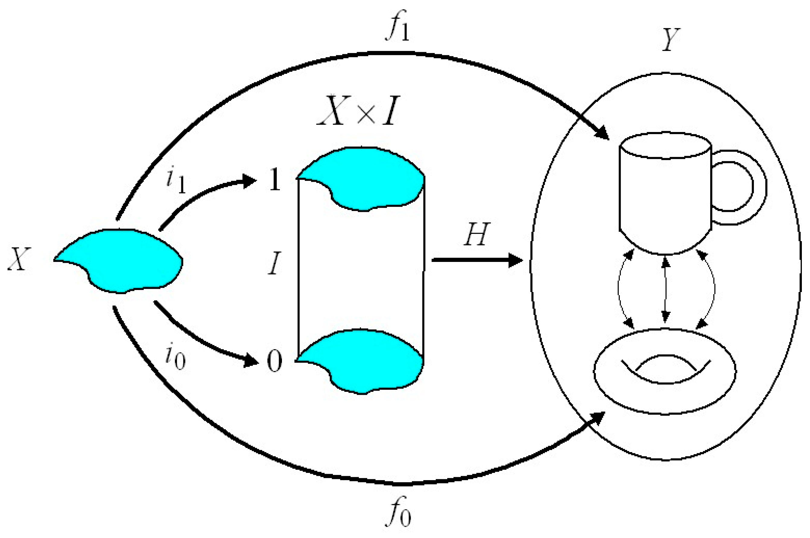
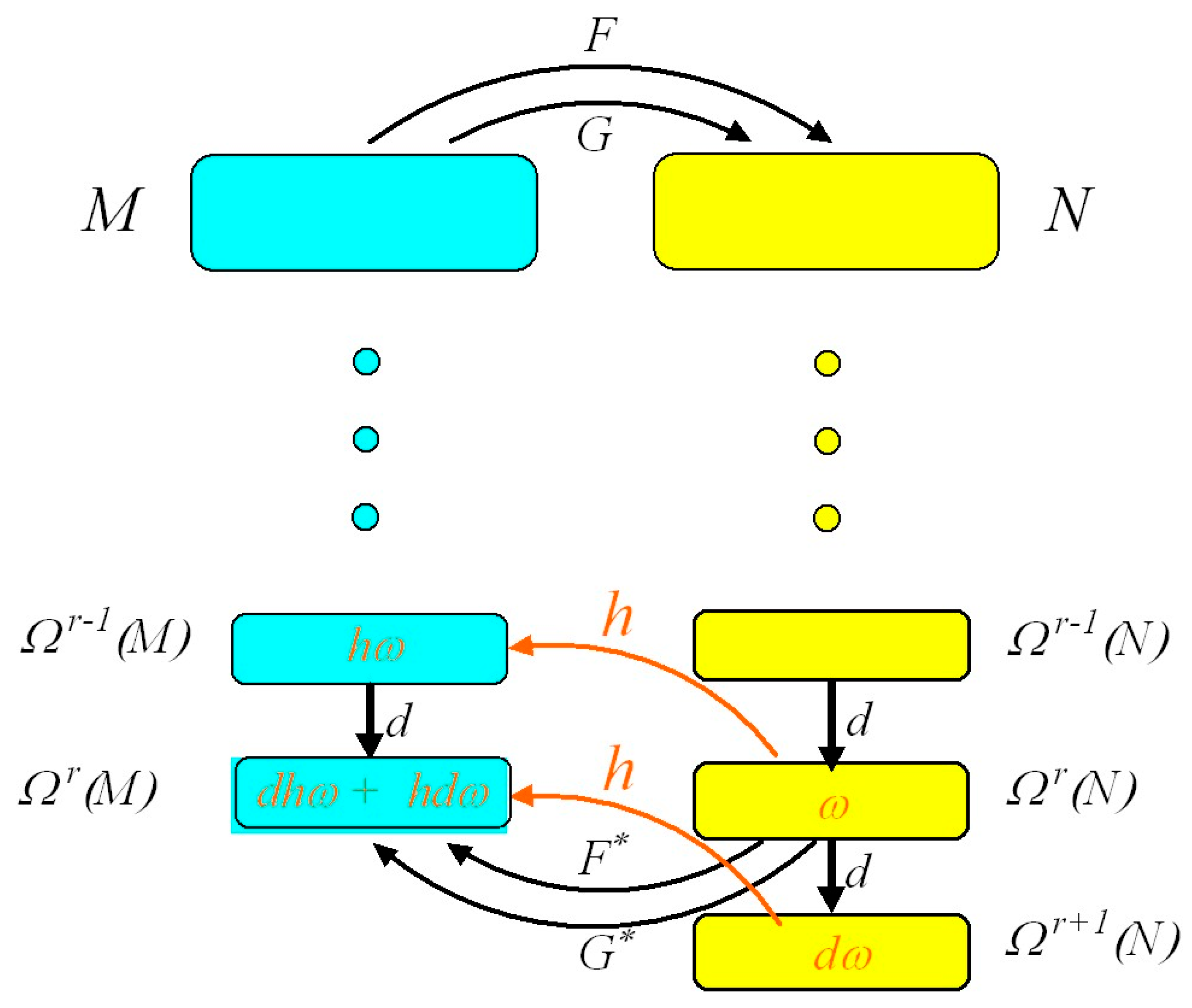
Disclaimer/Publisher’s Note: The statements, opinions and data contained in all publications are solely those of the individual author(s) and contributor(s) and not of MDPI and/or the editor(s). MDPI and/or the editor(s) disclaim responsibility for any injury to people or property resulting from any ideas, methods, instructions or products referred to in the content. |
© 2024 by the authors. Licensee MDPI, Basel, Switzerland. This article is an open access article distributed under the terms and conditions of the Creative Commons Attribution (CC BY) license (https://creativecommons.org/licenses/by/4.0/).