Abstract
We coin the term “network goodness” for a value we define for a network embedded in a given environment as a metric that describes the suitability of that network for meeting a demand. Three formulas are proposed to calculate the metric from three variable values. The first variable considers parts of the environment gravitated by the network. For these parts of the environment, we define a value that measures user costs refusing them the use of the network. Last but not least, the network maintenance costs are considered. The results are obtained after focusing on infrastructure and transport networks, but can be used for other types of networks as well.
1. Introduction
A network is designed to meet the demands of a specific environment. There are three essential factors to consider when evaluating a network in any environment:
- -
- The coverage range of the network within the environment;
- -
- The availability of the network for users, as reflected in the costs incurred by the user;
- -
- The maintenance costs associated with the network.
If the demand exceeds network capacity, some areas may not be serviced, service may become more expensive, or maintenance expenses may increase. Also, several networks may be embedded in the same environment to serve an environment’s demand.
In order to evaluate the function of a network, in this paper, we defined the “network goodness” function and propose formulas for calculating goodness values and comparing two or more infrastructure networks embedded in the same environment. We also thoroughly prove all theorems, propositions, lemmas, and corollaries, since no similar approach has, to date, been conducted in the available literature.
Currently, the predominant term used for evaluating network function is “Quality of Service” (QoS), and many millions of papers have been published on the subject over the years. A recently published work by Kanellopoulos et al. in [1] offers an extensive survey of network architectures and protocols. However, the authors only present a qualitative comparison of network requirements for some Smart City Applications (SCAs) and do not attribute an overall score that would enable ranking amongst the alternatives. Karakus and Durresi wrote an exhaustive survey paper [2] for comprehensively examining QoS in Software-Defined Networking (SDN)/OpenFlow networks. The authors provide a detailed overview of the SDN architecture and divide 43 different methods according to two approaches for maintaining the ability of a network to provide the required services for a selected traffic scenario. While it is clear that the soft Quality and Outcomes Framework (QoF) outperforms the hard QoF approach, no quantitative metric is defined.
In other works, network embeddings are discussed in terms of solving complex problems once a network is defined. In [3], Social Network Analysis (SNA) is presented as a powerful technique for building and maintaining social relationships within the network. In social networks, users interact and communicate with one another and also post personalized content. Novel Dynamic Attributed Network Embedding (DANE) is experimentally studied in [4] to advance learning tasks such as node classification, network clustering, and link prediction. Network embedding leverages node proximity to learn a low-dimensional node vector representation for each node within the existing social network, and hence studies how social relationships are established and evolve. However, the SNA values are also only given qualitatively, as DANE is evaluated. In [5], Salkhi et al. consider networks as a means of evaluating structural isolation and node integration, assessing their accessibility and navigability within the graph, and predicting potential structural changes that may impact the network’s evolution. However, again, no quantitative value is provided to measure either isolation or integration in the given scenario.
The application area we choose to showcase our approach is public transport networks. Typically, traffic infrastructure networks emerge naturally as demand increases in an environment. However, an existing network cannot meet the environment’s needs in time. In the last section, we presented several alternatives for public transportation routes that could accommodate a transportation mode with sufficient volume and speed to make public transport as attractive as possible. Despite searching the available literature, we could not find an instrument for quantitatively selecting heuristically drawn variants.
Bogdanova et al. investigate the transport facilities of a comfortable urban environment in [6], where the “network comfort” is measured by the number of users with less than 500 (or 800) meters to travel among the total population. The security rating of the public transport network is calculated by dividing the number of citizens injured in public transport by the total number of passengers using it. Transportation systems have become increasingly vital to modern economies, as Colon et al. describe in [7]. In [8]. Guliot proposes a decision tool that offers several alternative scenarios for reconfiguring transit services. Each scenario includes a set of existing lines to be closed and the corresponding delay profile caused by the closure of each line. Another study, by Wang et al. [9], addresses the unbalanced urban development by improving transportation efficiency, reducing traffic congestion and accidents, and coordinating transport transport. Kuo et al. in [10] emphasize the importance of readily available public transportation that provides real-time demand, offers convenient and high quality service, and operates in an energy-efficient way. In [11], Nes et al. present an optimization model for selecting routes, assigning frequencies, and determining the number of passengers on the existing network by generating a set of possible routes.
The rest of this paper is organized as follows. In Section 2, we introduce our terminology and outline the methodology, including lemmas and theorems and their proofs that underscore our approach. In Section 3, we present results and discuss them. In the following section, we offer an example of our proposed approach (Section 4), and in the final section, we offer conclusions (Section 5).
2. Terminology and Basic Theory
In this section, we define the terms we then use in theorems and lemmas. We draw our terminology from the fields of set theory, graph theory, and analytic geometrical calculus. First, we assume that any environment is within some “ground”: a state, a continent, or the Earth overall. The ground is a two-dimensional plane.
Definition 1
(Network environment and size). Network environment is part of the ground defined uniquely by its administrative borders or in any other unique way that determines which locations are within and which outside the ground. The area of is denoted , and is measured in squares.
The network environment is divided into zones comprising demand points where demand is concentrated. Different zones do not share the same demand point(s): mathematically, they are mutually disjointed.
Definition 2
(Demand zone and demand point). Demand zone is part of the network environment: . Further, for all , and for .
Demand point is a point with positive associated value , which is the demand concentrated at .
The number of demand points is , and it varies from zone to zone. The formal definition is given below.
Definition 3.
Suppose that for each there exists , and a finite set with injective function , denoted , and when . Then, is the demand quantity given in demand point denoted .
To calculate the network goodness, we require coordinates, a pair of numbers that uniquely determines the position of a point on the plane.
Definition 4
(Coordinated network environment). An environment is coordinated if any point can be uniquely defined by a pair of real numbers .
The coordinates are necessary for algebraic calculations, and we guarantee this by proving the following Lemma.
Lemma 1.
Any network environment can be coordinated.
Proof of Lemma 1.
We set a well-known location in the environment as a pair . We set the west–east direction through as the abscissa and the south–north direction as the ordinate axis. Then, any point is uniquely defined by pair . Usually, it is . □
Our objective is to evaluate a network, and for this we need to algebraically define a “segment” between two points.
Definition 5.
A segment between two points, A and B, with coordinates and , respectively, is a set consisting of all the points on the straight line connecting the two points.
In graph terminology [12], a graph is a pair defined by a given set of nodes N and a set of edges E given as a relation, . This means that E is a set of pairs taken from the set of all the possible pairs of all the nodes given in N. In our paper, a network is a connected graph , where E is a set of segments and N is a set of their endpoints. Because , a network is defined correctly, and we prove it formally in the following theorem, where .
Theorem 1.
Any set of segments defines a graph.
Proof of Theorem 4.
For a given set of segments , we denote every segment as an element in the set of edges , with . Further, each segment gives two points into the set of nodes with elements, since different segments may have one endpoint in common. Then, the given segments set generates with , in the well-known graph definition sense. □
A path is a sequence of chained segments. Path segments are considered chained if one segment endpoint matches the starting point of the next segment or the ending point of the path: . In Figure 3, a path is illustrated. We need the path term for the following definition.
Definition 6
(Connected graph). A graph is connected if any pair of nodes has a path that begins at one and ends at the other node.
The concept of a connected graph is necessary to define a network in our paper, as not every graph is a network. Definition 6 leads us to define the network we evaluate in our paper, which is given below.
Definition 7
(Network). A network is a connected graph consisting of a set of segments.
In the following theorem, we prove that each segment defined by Equation (1) corresponds to a unique equation derived from the segment’s boundary points.
Theorem 2.
We let and be points given in an environment covered by a coordinate grid. Then, segment is defined as set
Proof of Theorem 2.
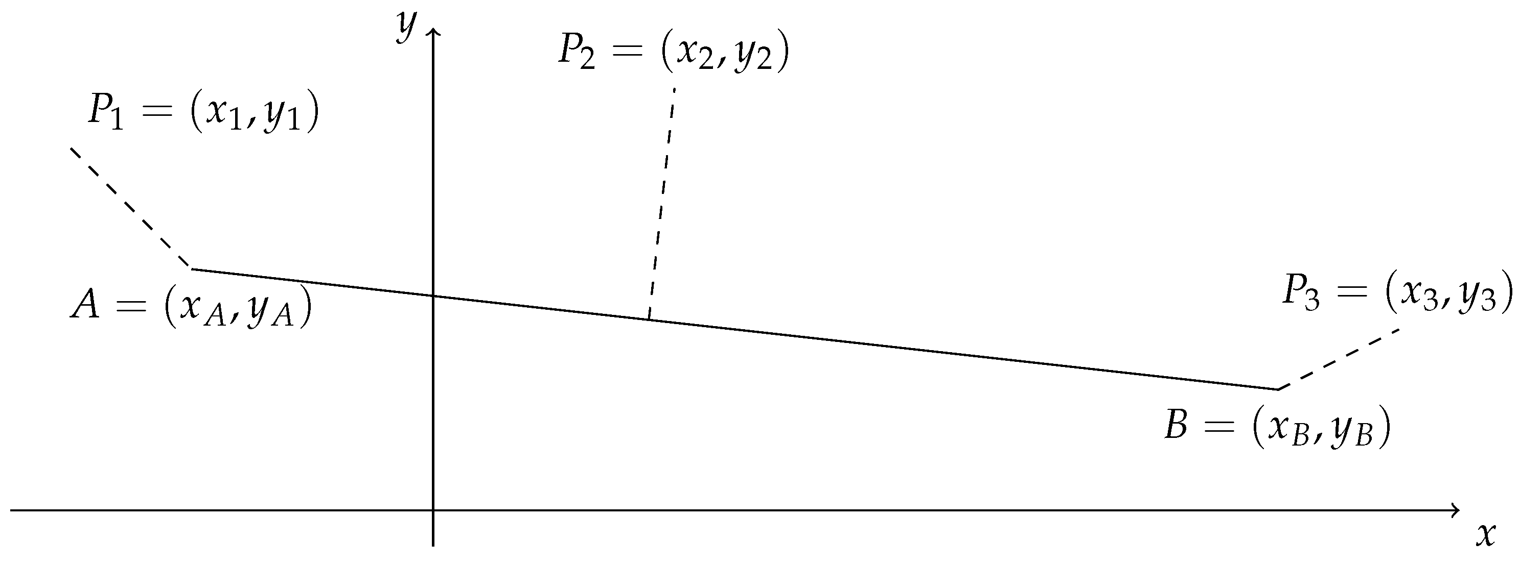
Figure 1 illustrates the positions of different points outside the segment concerning it. Having proven Equation (2), Theorem 2 enables us to calculate the square distance between a point and a segment. In the following theorem, we derive the square distance formulas for the position of each point depicted in Figure 1.
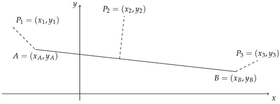
Figure 1.
Distances from the segment related to demand zones positions.
Theorem 3.
The square distance between point and segment is given by
or
in any other case.
Equation (5) is obtained after we define as the linear combination of vectors and , representing the unit steps in the east and north directions, respectively. Then, vector is given by
where and are already defined. The cosine of angle , with the vertex at A, is given by formula
Here, we note that , and . Furthermore, for , and for .
In addition, we take cross-product with and area . Namely, is a vector perpendicular to and , so it does not belong to the environment ground. Then, the Theorem 3 proof follows. More details about vector products can be found in [13].
Proof of Theorem 3.
In the case where , we have , and then Equation (3) is valid. If , then , and Equation (4) is valid.
In other cases, we equate the areas of triangle calculated using two approaches,
where the vector product is calculated in a three-dimensional space after environment is embedded in the sense . The absolute value on the right-hand side in Equation (8) equals
because area On the left-hand side of Equation (8), we have
Substituting Equations (9) and (10) into Equation (8), we obtain (5) after tidying up. □
In Definition 2, we define a demand point as a point with a positive number assigned to it that represents the demand at that point. It is important to note that not every point has a demand value. According to Definition 2, a demand zone contains only a finite number of demand points. If a point in the demand zone has no demand, it is not a demand point.
3. Results and Discussion
In this section, we explain the basics of our theory, starting with the zone demand center. Each demand zone has a unique demand center point. This point is calculated similarly to the center of gravity calculation in physics. Here, the calculation is given as a theorem that follows.
Theorem 4
(Zone demand center). Each demand zone has a unique demand center point with coordinates , calculated using formula
where is the total zone demand concentrated at .
The number of demand points within depends on , and thus it is denoted .
Proof of Theorem 4.

We prove the x-coordinate calculation from Equation (11) taking points and from Figure 1. If we suppose that mass , then , , and their center of gravity are positioned on the abscissa axis as shown in Figure 2.
Figure 2.
Calculating the two-demand-point demand center.
The center of the “teeter” in Figure 2 must satisfy the following “balance” law:
According to Equation (12), the center of gravity abscissa position is
Next, we extend the calculation to include . Supposing , we obtain the center of gravity between (13) with and with :
Proceeding, we obtain a penultimate center of gravity:
Together with the last demand point, we reach Equation (11) (this procedure is commonly termed “a pondering average”). □
The square distance between the demand zone and the network is the minimum square distance between the demand zone center and a network segment. The following theorem guarantees existence and uniqueness.
Theorem 5.
For a given network , and for each , where , there exists
In the proof below, we show induction as a suggestion for program applications. In the Example section, we use only the Excel tool to calculate the minimum distance, although the number of segments and zones is large.
Proof of Theorem 5.
Because the network is finite, the minimum distance always exists. Next, we perform induction by index j, .
For induction basic , we have . For , we take .
For step , we suppose that for graph there exists .
If , we separate , and then we have
for each . It has been proven that a square distance exists for each zone with a demand center at point . It is unique because if the minimum exists, it is always only one value. □
Next, we introduce the “inertia” of the demand zone. We remind that in the overall concept of network goodness, a higher score indicates better network service within the environment.
To determine the network goodness, we calculate the inertia of the demand zone that “gravitates” to the network. The inertia of a demand zone is determined by multiplying the zone’s demand with the minimum square distance between the demand zone center and a network segment. We formulate the inertia of a demand zone using the following definition.
Definition 8
(Demand zone inertia). The inertia of the ith demand zone is product
where is calculated from Equation (16) and is calculated in Theorem 4.
It should be noted that not all zones where there is demand for network service are considered when calculating the system’s inertia. To use the network service, their users must connect to the network independently.
In an infrastructure network, two types of distance influence a user’s choice of network for a service. A short distance attracts the user to choose the proposed network over other options. For instance, if a bus stop is close to someone’s apartment, they would only use the bus instead of their vehicle. Conversely, a greater distance is a limit beyond which the user will use the given network indirectly. In the following definition, we formally define both types of distances: gravitating and attracting distances and zones.
Definition 9
(Gravitating and attracting zones and distances). Demand zone , where , gravitates to the network iff for gravitating distance D, which is a value determined in advance.
Demand zone , with , is attracted by the network iff for an attracting distance d, which is a value determined in advance, too.
Further discussion of d and D related to public transport networks can be found in [14]. The value of D represents an acceptable distance of up to two kilometers that one can walk to reach the network. At the same time, d is the distance of a few hundred meters that a user is willing to walk instead of using any different mode of transportation.
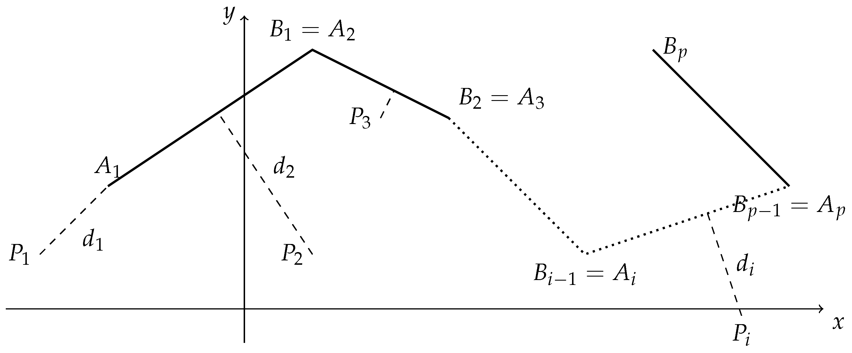
The total inertia of a network is the sum of the inertia of all gravitating demand zones. The quality of a network is determined by how low its network inertia is. A simple example is illustrated in Figure 3.
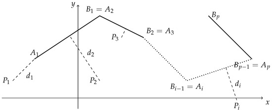
Figure 3.
Calculating the moment zone inertia along the path in a network.
Definition 10
(Network inertia and gravitating zones number). The network inertia is calculated by adding up the inertia of all the gravitating zones in the network.
There are k demand zones that gravitate towards the network, each represented by .
The total length of a network is the sum of its segment lengths.
Definition 11
(Network length). For a given network , the length is
When calculating the goodness of a network, we take into account three essential factors: the number of gravitating zones (k), the inertia (M), and the length (l). A network is considered good if it has as many zones connected and its inertia and length are as small as possible.
Next, we provide a weak definition for a network goodness function formula necessary for proving the propositions as our main results.
Definition 12.
A network goodness function of three variables is properly defined by a formula if it increases as k increases and decreases as l and M decrease.
When properly defined according to Definition 12, the value of the network goodness function provides a quantitative network evaluation in the sense that two or more networks embedded in the same environment are ranked such that a network with a higher goodness value is the “better”.
We propose three formulas that increase with the number of gravitating zones and decrease with the length and inertia of the network. They are presented in the order they were developed and have the same proof because increasing and decreasing are governed by positive and negative partial derivatives, respectively.
Proposition 1.
If k zones are attracted towards the network, and the network has an inertia of M with a length of l, then the network goodness function is given by formula
Proposition 1 outlines how Equation (20) quantifies the goodness of the network by Definition 12. Next, we discuss the powers attributed to l and k in (20). We note that the dimension of in the denominator is the same of that of M, that is, . The nominator highlights the number of gravitating zones, comparing it to the denominator’s value degrees. Namely, is in degree two, but M from (18) is in total degree three since it is obtained by multiplying demand with square distance. In accordance with Definition 12, Equation (20) defines a correct goodness function in three variables: , and l.
The partial derivatives of Equation (20) are given by
Because the network length is usually longer than half a kilometer, from Equations (21)–(23), the next inequality holds:
Proposition 2.
Given k, M, and l from Proposition 1, the network goodness function can be expressed using the following equation:
In the following, we offer the partial derivatives of the function in (25):
These lead to the following inequalities:
Proposition 3.
We let , and l be given as in the previous propositions. We let d and D be positive values from Definition 9 and let be calculated as in Theorem 4.
In the given environment, n represents the total number of demand zones that the network aims to serve. Then, the network goodness function is defined by equation
Equation (27) is dimensionless. This is particularly valuable when all demand zones gravitate attractively toward the network in the sense of Definition 9. Taking into account the values of and the total demand value , the following result validates the use of Equation (25) in the network goodness function.
Corollary 1.
If , , and for each , then the value calculated by Equation (27) is equal to one, that is, .
Proof of Corollary 1.
If conditions in Corollary 1 are fulfilled, then we say that the network is available with distance D and attractive with distance d. Next, we prove all the propositions.
The proofs of Propositions 1–3.
In the sense of Definition 12, the proofs of all the propositions are the same since the basis requests are satisfied. Following (26), all values , and g increase with k and decrease with l and M, as required. □
In Equation (27), the power in is used because in our Example section when . Cube is used because in our example, when .
To avoid confusion that may arise from the appearance of square and cube exponents in Equations from (20) to (27), we add the following theorem that uses ceiling function of an actual number x to determine the lowest integer greater than or equal to x.
Theorem 6.
We let values be as in Proposition 1 and let and be as in Proposition 3. We define α and β as follows:
If , then the value of function
depends increasingly upon k and decreasingly upon l and M. Depending on arbitrary values for d and D, may be lesser or greater than 100%.
Proof.
Again, partial derivatives . □
In the next section, we propose a Public City Transport (PCT) corridor network. The method combines environmental physics and social observations, behavior statistics, and heuristics, and applies the proposed theory to evaluate several network variants.
4. Example
Urban transport is a crucial pillar supporting citizen mobility in cities experiencing population growth and territorial expansion. Private transport tends to congest urban traffic until it cannot connect locations within the urban area.
It is necessary to invest in new modes of public transport in order to attract inhabitants to use it thanks to its availability, speed, and capacity. New modes need new corridors. Below is an example of the proposed procedure for the heuristic design and evaluation of public city transport corridor networks proposals. In the following, we demonstrate the process step by step.
The initial aim was to propose a network for the public transportation mode with large capacity and velocity. Usually, networks are embedded using the spanning tree or the least square method, but we proposed a network after several heuristically drawn variants and chose the best one. In the previous section, we proposed several functions for calculating the goodness of a network embedded in an environment for serving the users’ traffic demands. In this section, we applied them to compare several network variants obtained heuristically following exhausting statistical investigations.
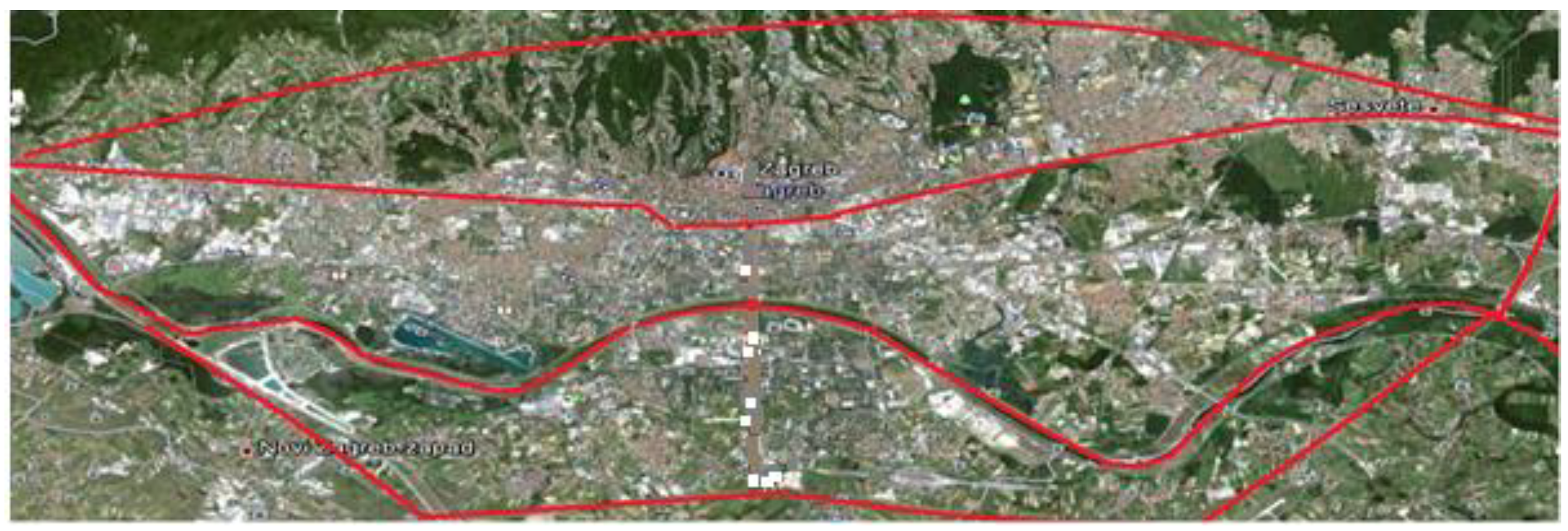
The primary prerequisite was to consider the natural obstacles in the environment. In Figure 4, four red barriers in the City of Zagreb are depicted, from north to south: the mountain, the railway, the river, and the highway.
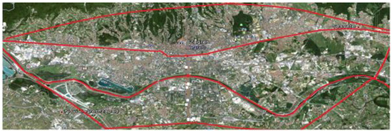
Figure 4.
Zagreb City County natural environment.
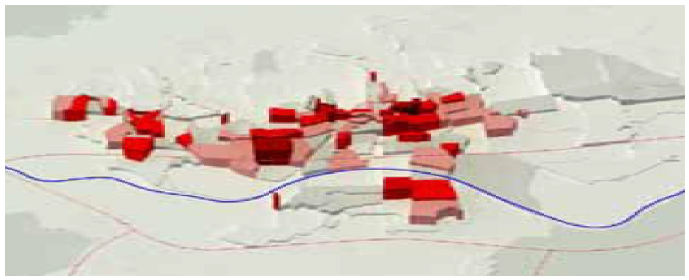
The zone partition was adopted from the former administrative local communities division and is shown in Figure 5. Demand points are buildings, schools, supermarkets, and other places where people can appear. Demand is the number of inhabitants or users taken from various reports. Demand centers are calculated by (11) after the coordinate system was established, according to Lemma 1. It is also necessary to calculate the moment inertia.
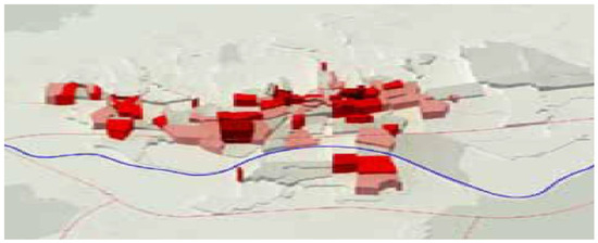
Figure 5.
Zagreb City local population centers. The darker the red color the larger the population at that location. Source: ZagrebPlan [15].
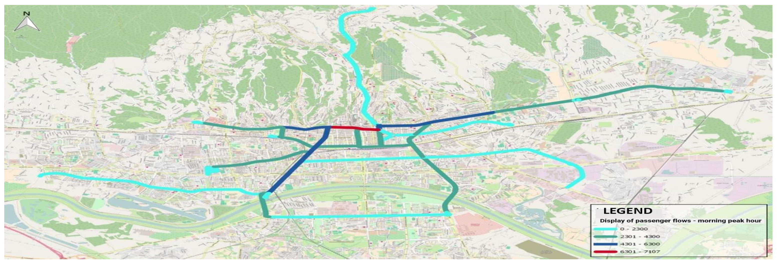
Once the environment was partitioned (see Figure 5), and taking into consideration the barriers shown in Figure 4, we sketched corridors composed of segments (see Equation (1)). The segments were embedded according to the main traffic flow directions. Flow directions were obtained after statistical monitoring and are presented in Figure 6.
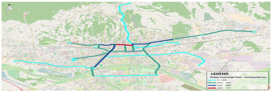
Figure 6.
Zagreb City passenger flows.
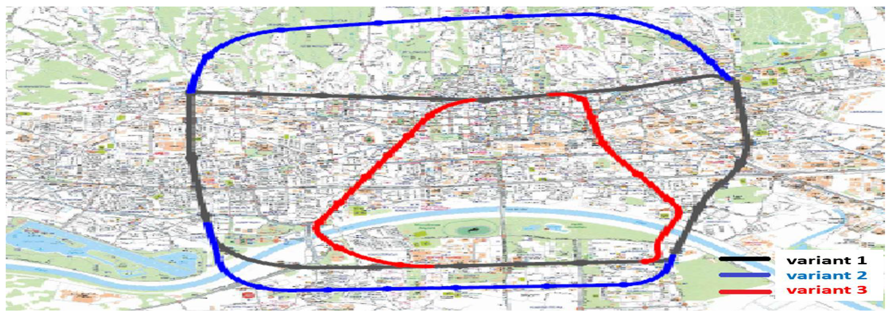
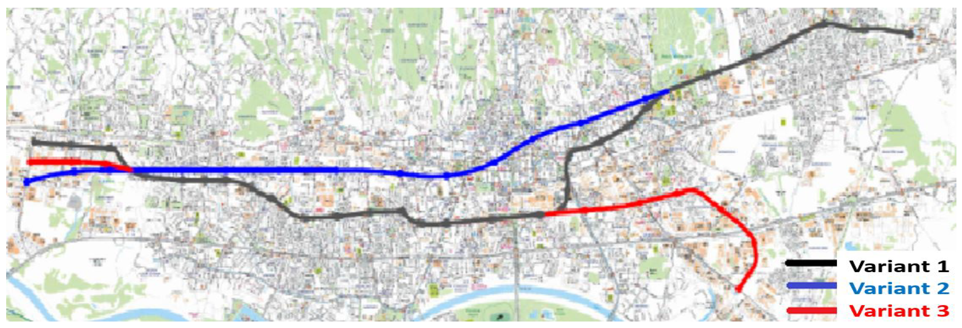
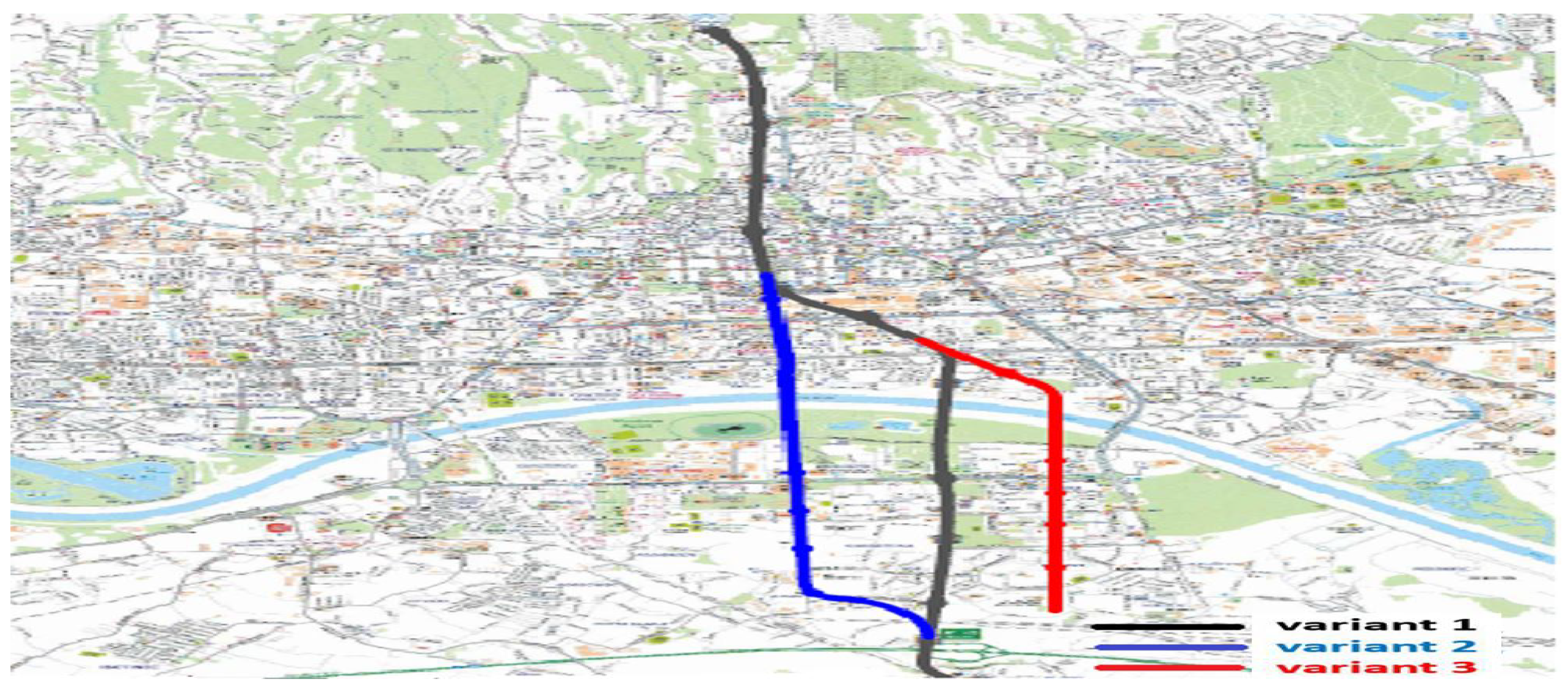
The heuristic design process was guided through the nine corridor network variants presented in Figure 7, Figure 8 and Figure 9. The network inertia for each of them was calculated according to Equations (17) and (18).
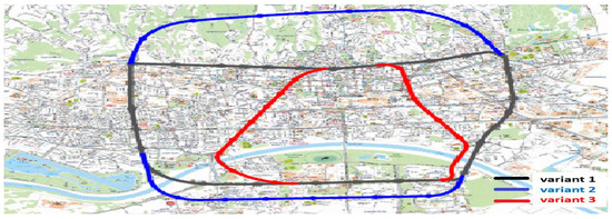
Figure 7.
The first proposed corridor network variants.
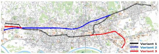
Figure 8.
The second proposed corridor network variants.
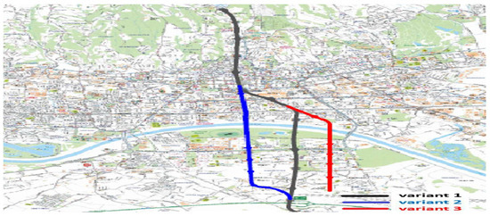
Figure 9.
The third proposed corridor network.
The variants of the corridor network in Figure 7 are drawn in a circle, relying on the flows from Figure 6. Only zones up to km are observed as the gravitating zones for inertia calculation.
The variants in Figure 9 are drawn according to the north–south directions in Figure 6. New, modified corridors imply consideration of Figure 5.
The corridors in Figure 8 stretch in the west–east direction following the flows from Figure 6. Then, these directions are connected with lines in the north–south direction. The process continues by considering the west–south direction in Figure 6. A good public traffic network attracts citizens to use the public traffic network rather than private transport devices if it is created to reduce the amount of walking necessary, as expressed by network inertia (see Equation (18)).
The formulas proposed in Propositions 1–3 were used to quantitatively compare different corridor networks, considering network availability through the number of gravitating demand zones and network costs roughly proportional to network length.
In the city of Zagreb, the environment area size is , the traffic demand is = 680,000, and the total environment parts number is n = 160. Values d = 200 m and D = 4 km were taken following the recommendations in [14].
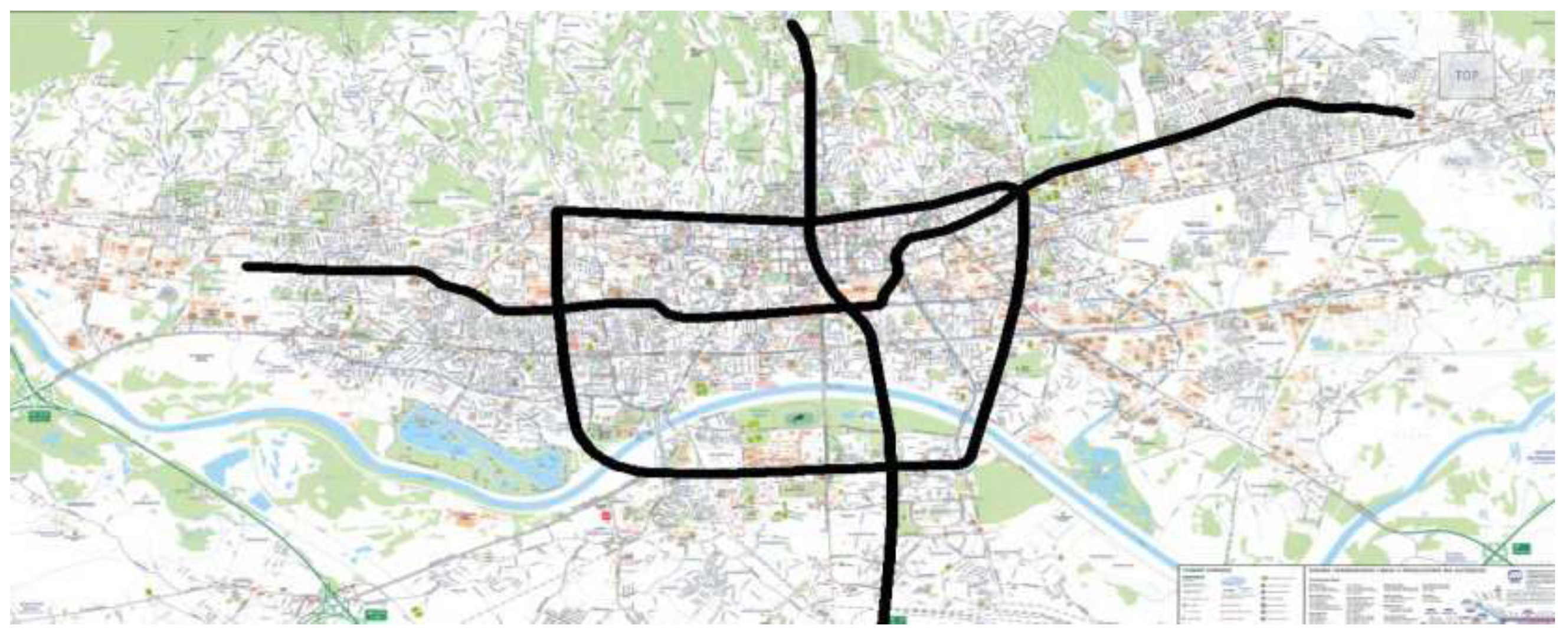
In Figure 7, Figure 8 and Figure 9, three kinds of variants are proposed, according to the passengers’ flow directions from Figure 6. In Table 1, goodness values for each variant are listed, and the best variant’s goodness values are considered. Then, we collect the final network in Figure 10 by taking the first variants from Figure 7 and Figure 8, and the third variant from Figure 9.

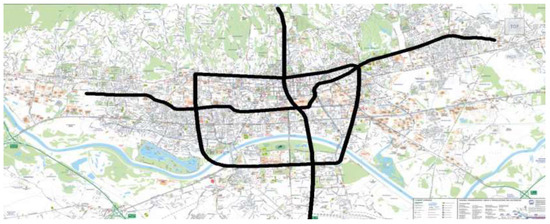
Figure 10.
The final proposed corridor network variant.
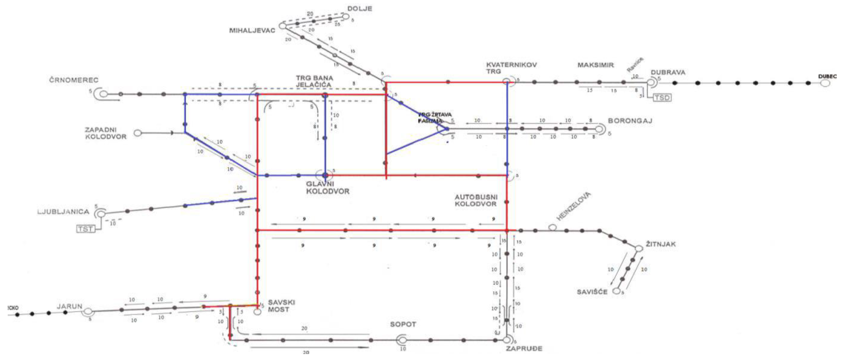
For comparison, we calculated values for the temporary Zagreb Electrician Tramway network given in Figure 11.
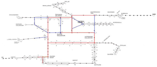
Figure 11.
ZET network that is existing. Source: Time table of the ZET branch (2020).
5. Conclusions
We offer mathematical expressions that quantify the goodness of different networks based on (i) coverage, (ii) availability, and (iii) maintenance expenses. Although the model is developed heuristically, we show it can be a reliable tool for assessing various networks suggested for embedding in an environment.
The ongoing discussion on using heuristics to create mathematical formulas involves using rules of thumb, intuition, and common sense to find a solution that is good enough and rapid. Heuristics from experience and intuition are sometimes better than exact methods or exhaustive simulation procedures. Moreover, if there is nothing similar in the literature available to evaluate a network quantitatively with a unique value, then the heuristic approach offers a good solution.
However, it is crucial to evaluate the results of heuristics. The first issue we tackle is selecting the best network variant among heuristically obtained variants. We propose several variants to solve the problem in Section 4 and justify our approach for choosing the best option.
Finally, we plan to develop this work further in the future.
Author Contributions
Conceptualization and validation, M.B.; methodology and formal analysis, B.I.; investigation, resources, and original draft preparation, M.P. All authors have read and agreed to the published version of the manuscript.
Funding
This research received no external funding.
Institutional Review Board Statement
Not applicable.
Data Availability Statement
Data sharing not applicable.
Acknowledgments
We thank the Krapina University of Applied Sciences and the Sami Shamoon College of Engineering for their moral support.
Conflicts of Interest
The authors declare no conflicts of interest.
References
- Kanellopoulos, D.; Sharma, V.K.; Panagiotakopoulos, T.; Kameas, A. Networking Architectures and Protocols for IoT Applications in Smart Cities: Recent Developments and Perspectives. Electronics 2022, 12, 2490. [Google Scholar] [CrossRef]
- Karakus, M.; Durresi, A. Quality of Service (QoS) in Software Defined Networking (SDN). A Surv. J. Netw. Comput. Appl. 2017, 80, 200–218. [Google Scholar] [CrossRef]
- Smit, L.C.; Dikken, J.; Schuurmans, M.J.; de Wit, N.J.; Bleijenberg, N. Value of social network analysis for developing and evaluating complex healthcare interventions: A scoping review. BMJ Open 2020, 10, e039681. [Google Scholar] [CrossRef] [PubMed] [PubMed Central]
- Li, J.; Harsh, D.; Hu, X.; Tang, J.; Yi, C.; Liu, H. Attributed Network Embedding for Learning in a Dynamic Environment. In Proceedings of the CIKM’17, Singapore, 6–10 November 2017. Session 2D: Network Embedding 2. [Google Scholar] [CrossRef]
- Salkhi Khasraghi, G.; Volchenkov, D.; Nejat, A.; Hernandez, R. University Campus as a Complex Pedestrian Dynamic Network: A Case Study of Walkability Patterns at Texas Tech University. Mathematics 2023, 12, 140. [Google Scholar] [CrossRef]
- Bogdanova, T.V.; Evdokimov, K.A. Transport component of a comfortable urban environment. Inov. Investments 2021, 2021, 163–170. [Google Scholar]
- Colon, C.; Hallegatte, S.; Rozenberg, J. Criticality analysis of a country’s transport network via an agent-based supply chain model. Nat. Sustain. 2021, 4, 209–215. [Google Scholar] [CrossRef]
- Guillot, M.; Furno, A.; Aghezzaf, E.; El Faouzi, N. Transport network downsizing based on optimal sub-network. Commun. Transp. Res. 2022, 2, 100079. [Google Scholar] [CrossRef]
- Wang, S.; Wang, Z. Collaborative Development and Transportation Volume Regulation Strategy for an Urban Agglomeration. Sustainability 2022, 15, 14742. [Google Scholar] [CrossRef]
- Kuo, Y.; Leung, J.M.; Yan, Y. Public transport for smart cities: Recent innovations and future challenges. Eur. J. Oper. Res. 2023, 306, 1001–1026. [Google Scholar] [CrossRef]
- Nes, V.R.; Hamerslag, R.; Immers, R. Design of Public Transport Networks. Transp. Res. Rec. 1988, 1202, 74–83. [Google Scholar]
- Wilson, R.J. Introduction to Graph Theory, 4th ed.; Longman Group Ltd.: Harlow, UK, 1996; Available online: https://www.maths.ed.ac.uk/~v1ranick/papers/wilsongraph.pdf (accessed on 20 February 2023).
- Lang, S. Introduction to Linear Algebra. In Springer Books on Elementary Mathematics; Springer: Berlin/Heidelberg, Germany, 1986; ISBN 978–1-4612-7002-7. Available online: https://www.math.nagoya-u.ac.jp/~richard/teaching/f2014/Lin_alg_Lang.pdf (accessed on 15 April 2024).
- Šimunović, L.J.; Ćosić, M. Osobitosti Pješačkoga Prometa. In Nemotorizirani Promet; Hrvoje Gold; Faculty of Traffic and Transport Sciences: Zagreb, Croatia, 2015; pp. 3–9. [Google Scholar]
- Available online: https://www.zagreb.hr/UserDocsImages/arhiva/zagrebplan-ciljeviiprioritetirazvojado2020.pdf (accessed on 12 December 2020).

Disclaimer/Publisher’s Note: The statements, opinions and data contained in all publications are solely those of the individual author(s) and contributor(s) and not of MDPI and/or the editor(s). MDPI and/or the editor(s) disclaim responsibility for any injury to people or property resulting from any ideas, methods, instructions or products referred to in the content. |
© 2024 by the authors. Licensee MDPI, Basel, Switzerland. This article is an open access article distributed under the terms and conditions of the Creative Commons Attribution (CC BY) license (https://creativecommons.org/licenses/by/4.0/).