Abstract
As photovoltaic (PV) deployment increases worldwide, PV systems are being installed more frequently in locations that experience snow cover. The higher albedo of snow, relative to the ground, increases the performance of PV systems in northern and high-altitude locations by reflecting more light onto the PV modules. Accurate modeling of the snow’s albedo can improve estimates of PV system production. Typical modeling of snow albedo uses a simple two-value model that sets the albedo high when snow is present, and low when snow is not present. However, snow albedo changes over time as snow settles and melts and a binary model does not account for transitional changes, which can be significant. Here, we present and validate a model for estimating snow albedo as it changes over time. The model is simple enough to only require daily snow depth and hourly average temperature data, but can be improved through the addition of site-specific factors, when available. We validate this model to quantify its ability to more accurately predict snow albedo and compare the model’s performance against satellite imagery-based methods for obtaining historical albedo data. In addition, we perform modeling using the System Advisor Model (SAM) to show the impact of changes in albedo on energy modeling for PV systems. Overall, our albedo model has a significantly improved ability to predict the solar insolation on PV modules in real time, especially on bifacial PV modules where reflected irradiance plays a larger role in energy production.
1. Introduction
Photovoltaic (PV) technologies are evolving rapidly, at both the cell level and the module level, resulting in significantly higher efficiencies and lower costs. In addition, PV systems are now being deployed in locations once thought to be unfavorable for solar-generated electricity. High-latitude locations, as well as other regions where snow prevails for many months of the year, are one example. Performance in these regions can be increased by installing PV modules at steeper tilt angles than are typical for middle latitudes [1,2]. Performance can also be increased by deploying bifacial modules, which receive irradiance from both the front and rear surfaces, resulting in higher electricity production and lower levelized cost of energy (LCOE) projections [3,4]. In high-albedo environments, for example, the amount of reflected light reaching the rear side of a module’s solar cells can increase the energy output by as much as 30 percent [5,6]. Given the energy gains and minimal price difference between bifacial and monofacial modules, bifacial modules now dominate the utility-scale market worldwide; moreover, they have driven the significant growth of utility-scale PVs in arctic regions, including Alaska [7]. The International Technology Roadmap for Photovoltaic (ITRPV) notes that by 2030, bifacial PV cells are expected to account for 70% of the total world PV cell market [8].
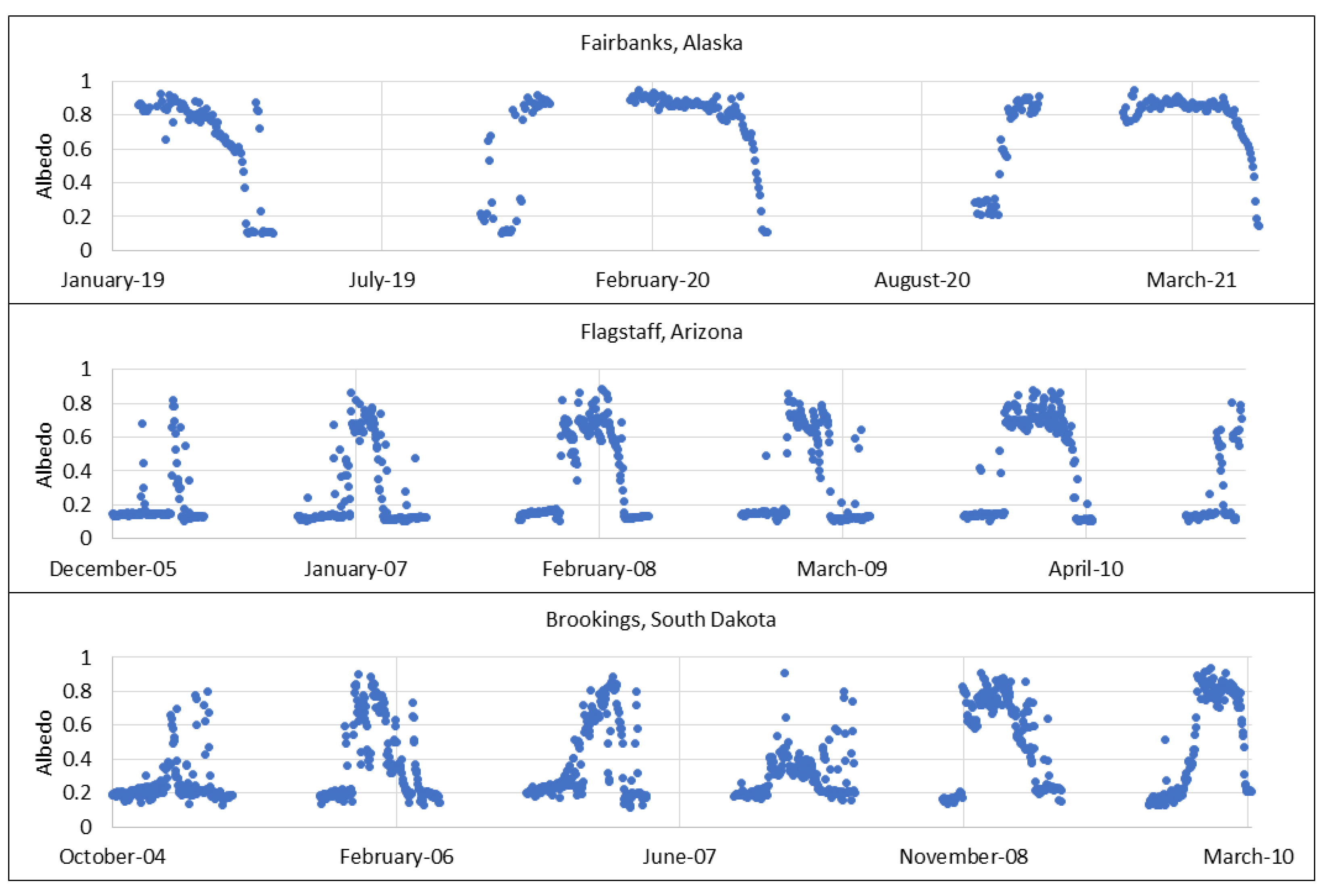
To accurately model the energy output of bifacial PV, rear-side plane-of-array (POA) irradiance data are needed [9], and ground albedo is an important input for modeling the amount of irradiance incident on the rear side of a PV module [10]. Accurate ground albedo measurements can also improve performance models for high-tilt-angle monofacial solar PV systems that are typically found at high latitudes [11] where ground-reflected irradiance can contribute to the irradiance incident on the front of the modules. Existing models typically assume an albedo of 0.8 if snow is present, and 0.2 if no snow is present [12,13]. This can lead to inaccuracies because the albedo of snow can vary drastically, depending on the age and characteristics of the snow [14], so the actual snow albedo at any point in time often lies between these two values. This is demonstrated in Figure 1 below, which tracks the winter-time albedo in Fairbanks, Alaska; Flagstaff, Arizona; and Brookings, South Dakota. Between October 1st and April 30th, albedo is between the 0.2 and 0.8 thresholds 32% of the time, 36% of the time, and 68% of the time, respectively, supporting the need for an alternative to the current 0.8 and 0.2 snow/no-snow albedo assumptions often utilized.
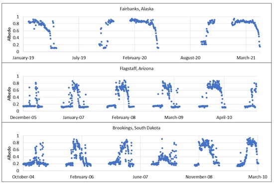
Figure 1.
Measured ground albedo at three different locations over multiple years, illustrating that the albedo is often between the default values of 0.8 if snow cover is present and 0.2 if snow cover is not present.
This work presents the following:
- A detailed description of our team’s multi-year analysis of time-series albedo data;
- A method to model the albedo of snow as a function of temperature and time since the last snowfall;
- A comparison of the performance of the developed model against existing common models for estimating ground albedo and remote sensing albedo measurements;
- Evidence showing that improved snow albedo modeling can improve the accuracy of PV performance models.
Historical Approaches to Modeling the Changing Albedo of Snow
Historically, albedo models have been included within climate change models or considered as offshoots of snow melt models [15,16,17]. As Dirmhirn and Eaton [18] note, the daily variation in albedo from snow-covered surfaces is attributable to the varying contributions of angle-of-incidence-dependent specular reflection from the snow surface as well as from the metamorphism of the snow based on temperature and time. For the albedo model presented in this paper, we authors were not concerned about short-term sun-angle-dependent changes in albedo but instead focused on daily albedo changes linked to snow metamorphism. This premise is well documented in the literature: Rango and Martinec [17], for example, note that older wet snow with a higher density has a lower albedo and a high liquid water content, and with each subsequent degree day becomes more melt-efficient. Anderson [19] similarly demonstrates the negative relationship between snow density and albedo. Since snow albedo changes as snow metamorphoses, and snow density changes during the melt process, we surmised that some of the same inputs for snow melt models could also inform a snow albedo model.
Particularly in recent decades, satellite-based irradiance measurements have been used to construct historical time-series albedo datasets for regions with significant snow cover for at least part of the year. Calleja et al. [16], for example, used data from the Moderate Resolution Imaging Spectroradiometer (MODIS) to examine the influence of incident radiation and ambient temperature on the snow albedo of a region of Antarctica. Jin and Simpson [20] used data taken from the U.S. National Oceanic and Atmospheric Administration (NOAA) Advanced Very High Resolution Radiometer (AVHRR) and an established model for transforming top-of-atmosphere and reflected irradiance into values for albedo and implemented two methods to correct for non-isotropic snow cover. Stroeve and Nolin [21] used data from the Multi-Angle Imaging Spectroradiometer (MISR) to generate snow albedo data over the Greenland ice sheet at a 1.1 km resolution. As discussed below, while albedo measurements from these sources can agree well with local ground measurements, their limited spatial resolution can potentially lead to inaccuracies in situations where albedo variation is highly dependent on local topography and micro-climates. Additionally, satellite imagery datasets tend to be published in batches at relatively infrequent time intervals, limiting their applicability to more-real-time modeling.
Snow melt models are common in the hydrology field and enable planners to predict water runoff and make water resource planning decisions. The need to understand and predict snow ablation extends from engineering applications to understanding the role of the Arctic in the global ecosystem [14]. Two types of snow melt models are generally adopted: the data-intensive surface energy-balance models and the relatively simple degree-day models [14,17]. Energy-balance models are sophisticated and the inputs include net radiation, sensible and latent heat flux, conductive energy flux, and the energy required to heat the snowpack to 0 °C [14]. Degree-day models (also referred to as the temperature index method) calculate snow melt depth by multiplying the number of degree days by the degree day ratio [17], and the work presented here is inspired by degree-day models. Amaral et al. [22] developed a similar albedo decay model using snow melt data collected in New Hampshire. However, Amaral et al. used a less-common snow density measurement as an input.
The melt-hour albedo model described herein presents a simple model for estimating the reduction in albedo of snow after a snowfall. The goal of this model is to maintain reasonable accuracy of the albedo prediction while minimizing the amount of input data and thus minimizing the barriers to its use. A more accurate estimate of snow surface albedo will enable PV performance modelers to improve the accuracy of their energy estimates. This improvement will be especially notable in high-latitude climates, which frequently utilize high PV tilt angles, as well as for bifacial PV modules which are becoming increasingly common in PV system deployments.
Within this paper, we first describe the data upon which the model is built, then describe how the model was developed from these data; we discuss the performance of the model, and then finally describe the impact of the model on improving the accuracy of PV system performance models.
2. The Melt-Hour Albedo Model
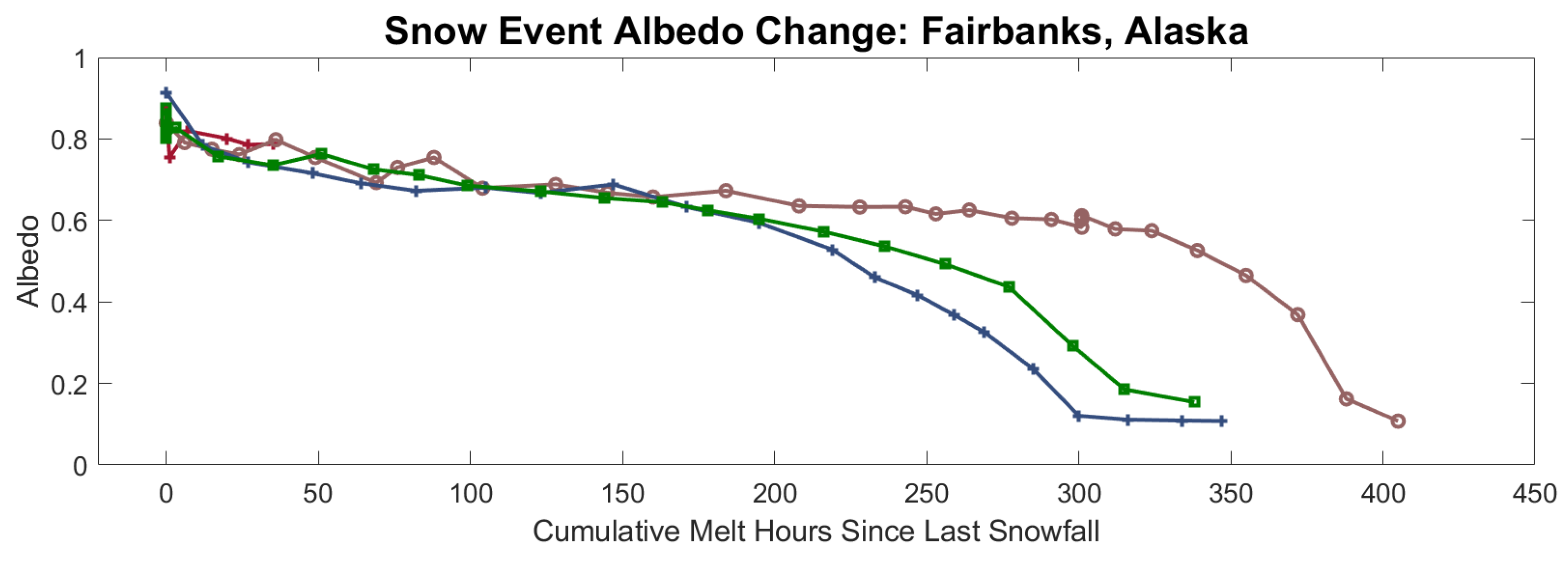
We refer to the model presented in this paper as the “melt-hour” albedo model. This model incorporates time and temperature by modifying the degree-day snow melt methodology referenced above. In this method, a melt hour is any hour with an average ambient temperature above 0 °C. For example, a day where 5 of the 24 h had an hourly average ambient temperature greater than 0 °C would generate 5 melt hours. Thus, each day has a maximum of 24 potential melt hours. Albedo can then be plotted as a function of the number of melt hours since the end of the last snowfall, as shown in Figure 2.
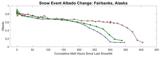
Figure 2.
The measured albedo as a function of the melt hours since the end of the last snowfall that was classed as a snow event, shown for snow events in Fairbanks, Alaska. Each curve denotes a different snow event.
We chose to incorporate hourly temperature evaluations (rather than average daily temperatures) into the model to enable a higher temporal resolution while still utilizing commonly available hourly temperature data. The alternative—the use of a single average daily temperature—would not have distinguished between daytime hours with temperatures above 0 °C and nighttime temperatures well below freezing. In such a scenario, the average daily temperature could be below 0 °C but several hours in the middle of the day could experience temperatures above 0 °C and melting would occur without being captured by such a model.
3. Data Acquisition and Preparation
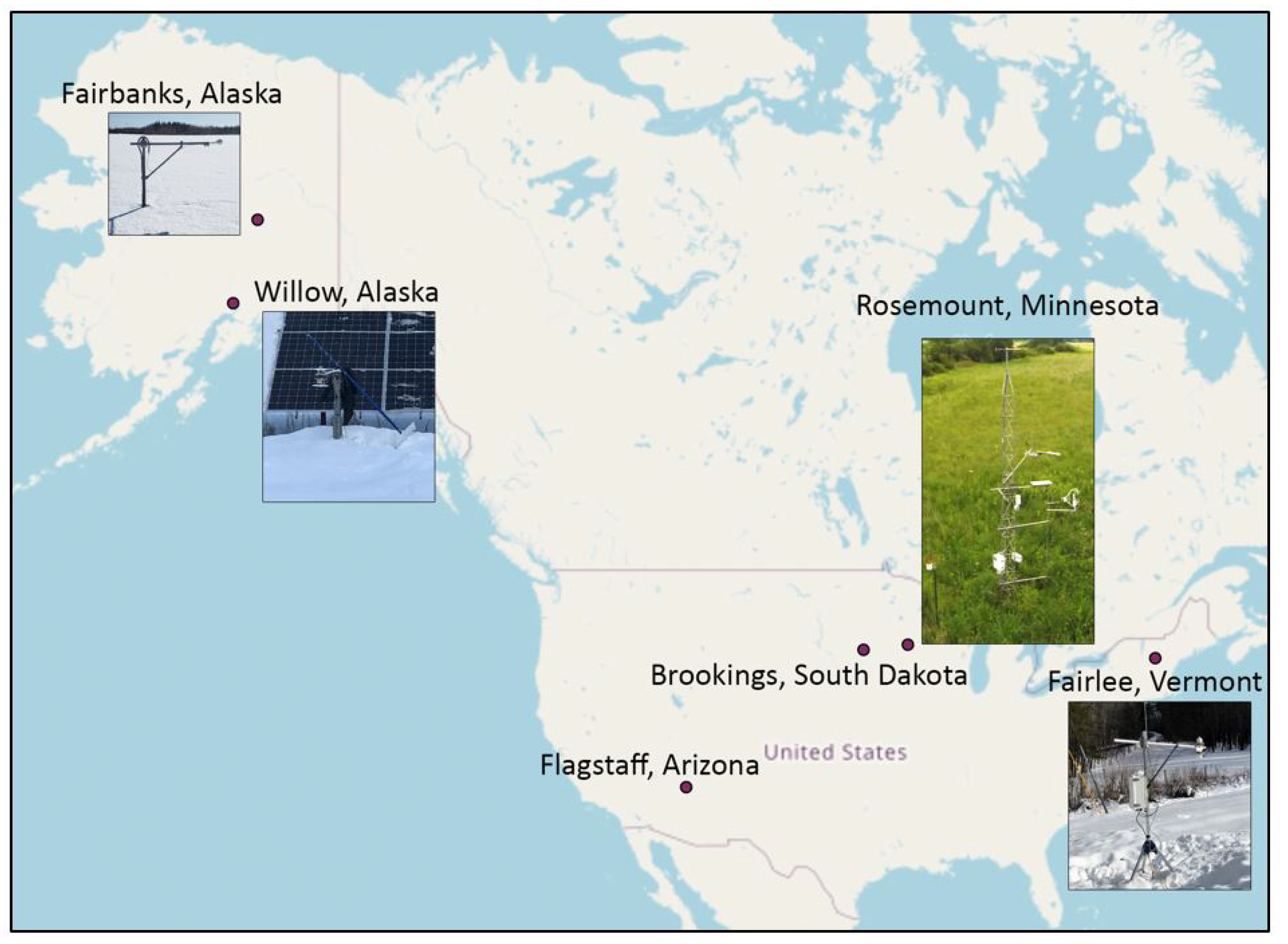
Data from six geographically diverse locations—Fairbanks, Alaska; Willow, Alaska; Fairlee, Vermont; Brookings, South Dakota; Flagstaff, Arizona; and Rosemount, Minnesota—were used to develop and train the melt-hour albedo model. The geographic diversity of these data collection locations improves the resulting model by aiding its applicability across various environments. Datasets from these locations included albedo, temperature, snowfall, and snow depth measurements. Albedo is measured via an albedometer, whereby irradiance is measured using an upward-facing and downward-facing pyranometer. The albedo is then reported as the ratio of the irradiance from the downward pyranometer to that from the upward pyranometer. Albedo and temperature were recorded at a minimum of one-hour resolution; and snowfall and snow depth data were recorded at daily resolution. Albedo data from the Alaska and Vermont sites were measured by the authors specifically for the development and validation of the proposed model, whereas the datasets for South Dakota, Arizona, and Minnesota (Figure 3) were downloaded from the National Renewable Energy Laboratory (NREL) DuraMAT website and are part of the AmeriFlux data network [23,24,25,26].
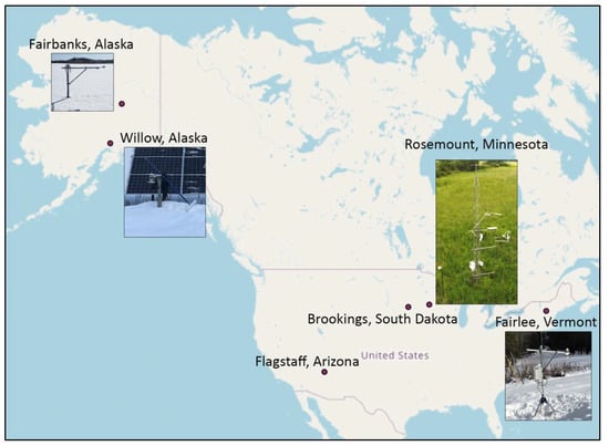
Figure 3.
Site locations of irradiance instrumentation that provided data for the melt-hour albedo model.
Snow coverage observations included daily snowfall amounts and snow depth on the ground, and were obtained either through on-site image acquisition or from the NOAA National Climate Data Center dataset closest to the albedo data collection site [27]. The exact location of the albedometer instrumentation and snow observations at each site is documented in Table 1.

Table 1.
Locations and temporal resolution of the six datasets used for developing the melt-hour albedo model.
The data-cleaning process included removing data that met the following criteria:
- Global horizontal irradiance (GHI) > 1200 W/m2;
- Reflected horizontal irradiance (RHI (reflected GHI that is measured with a downward-facing horizontal pyranometer [28])) > 1100 W/m2;
- -
- The maximum GHI and RHI figures were derived from testing performed at Sandia National Lab in Albuquerque, New Mexico [29] (See the Supplementary Materials).
- Albedo values greater than 0.95 [30] or less than 0.1 [31];
- -
- Past research suggests that albedo values outside these bounds are exceedingly rare and represent errors in the data.
- Albedo values measured when solar elevation was less than 5 degrees;
- -
- Quality control data filtering of irradiance data often flags data collected when the zenith angle > 80 degrees (10 degree solar elevation) in order to manage the effect of air mass [32]. This research chose to filter out data collected when the solar elevation < 5 degrees in order to minimize winter-time data losses at high latitudes.
- Albedo values measured more than one hour outside of solar noon;
- -
- Collecting albedo data around solar noon ensures consistency and minimizes the diurnal variation of albedo during low sun elevation angles [33].
- Other known shading or non-standard events.
4. Model Development
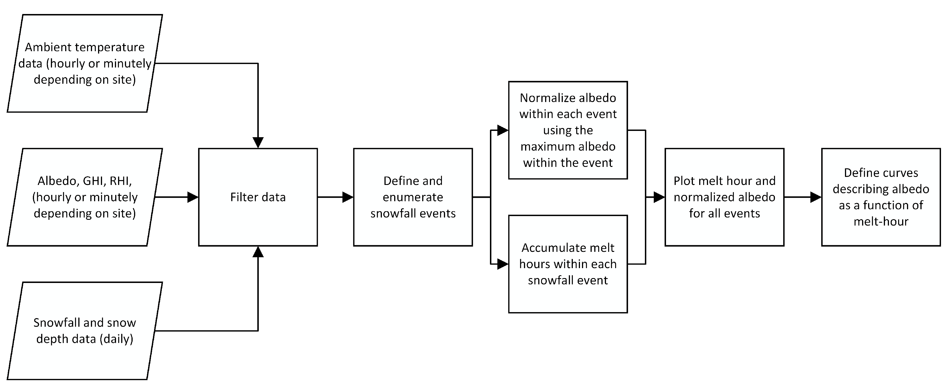
The development of the melt-hour albedo model is summarized in Figure 4, which shows the data inputs, described in the previous section, and the process we used to develop the model from those data. After the filtering described previously, we combined the average daily albedo and daily snowfall data to visualize how snow albedo changes over time and specifically how albedo changes after a snowfall. We grouped the data into “snow events” (or, alternately, “events”), where a snow event is defined as a time period of three or more days that make up the interval between the end of one snowfall and the beginning of the next snowfall, as exemplified in Figure 5 for Fairbanks, AK.
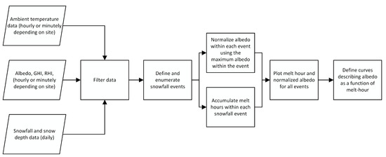
Figure 4.
Flowchart summarizing key steps of the albedo change model development process.
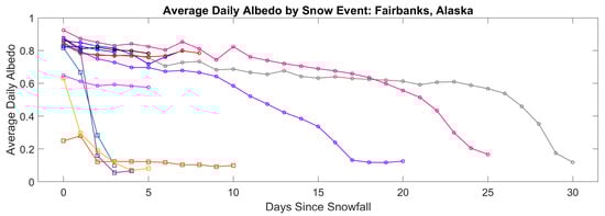
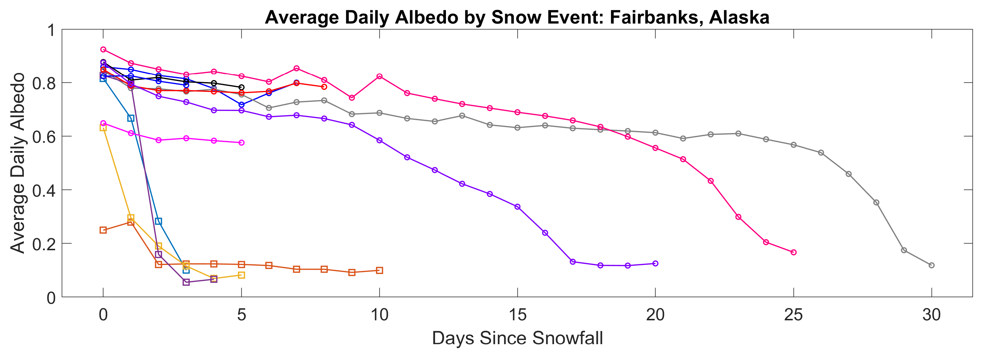
Figure 5.
Snow events, each one represented by a different color, recorded in Fairbanks, Alaska, shown in terms of the daily average albedo.
To observe the effect of time and temperature on albedo, we developed the melt-hour albedo methodology described above. We then incorporated the total number of melt hours into the daily albedo dataset so that each day was associated with the average daily albedo and the total daily sum of the melt hours. Then, events with melt hours equal to 0 were separated from events with melt hours greater than 0. To be more specific, during a snow event with a melt hour total of zero, the average hourly temperature would never have exceeded 0 °C.
Next, we applied an additional filtering step to remove events with maximum albedo values less than 0.5. Since freshly fallen snow typically has an albedo above 0.5, events with a maximum albedo less than 0.5 suggest either faulty data or incomplete snow coverage.
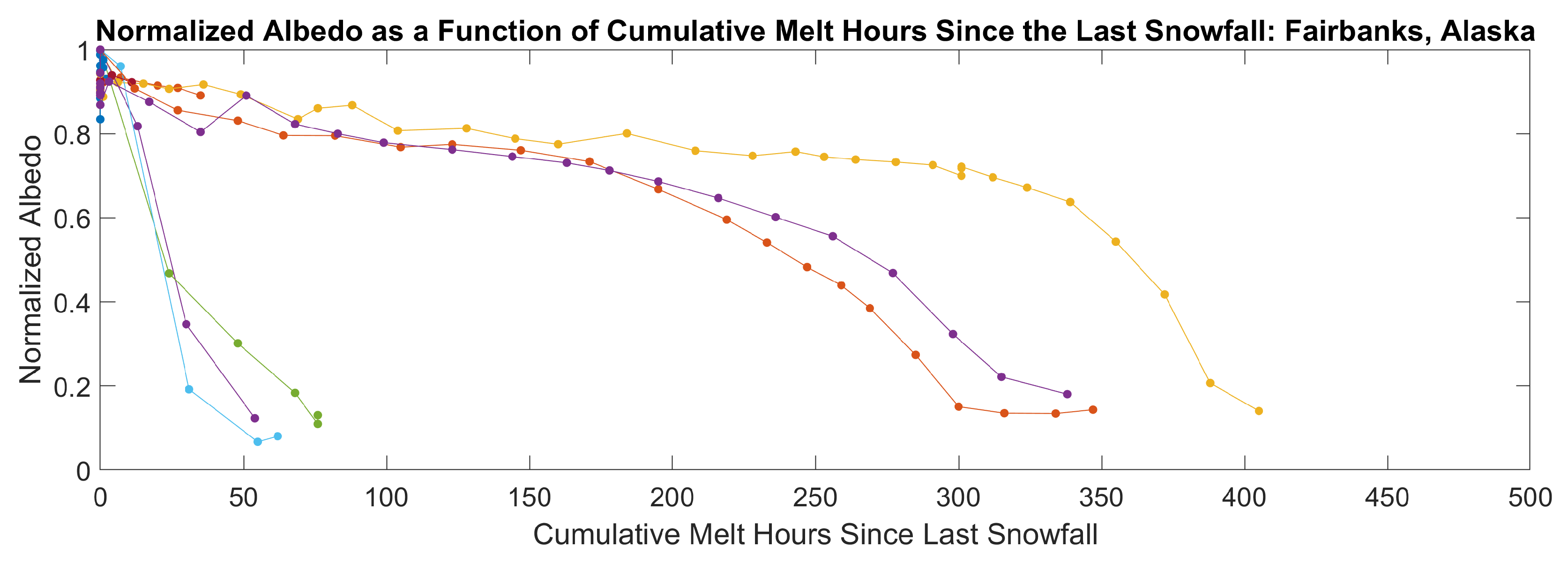
We then normalized all measured albedo values within each event so that the maximum normalized albedo within each event was equal to 1; this allows us to compare events and focus on the relative albedo change over time. Figure 6 shows the normalized albedo versus the melt hours since the previous snowfall using the data from Figure 5 to demonstrate how the melt-hour technique is useful for comparing snow events. This methodology is explained below and was used to develop the albedo change curves used in the model.
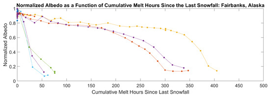
Figure 6.
Normalized albedo shown according to the cumulative melt hours since the last snow event, with each line representing a different event. Normalizing the maximum event albedo to 1 allows for the slopes of the events to be easily compared to one another.
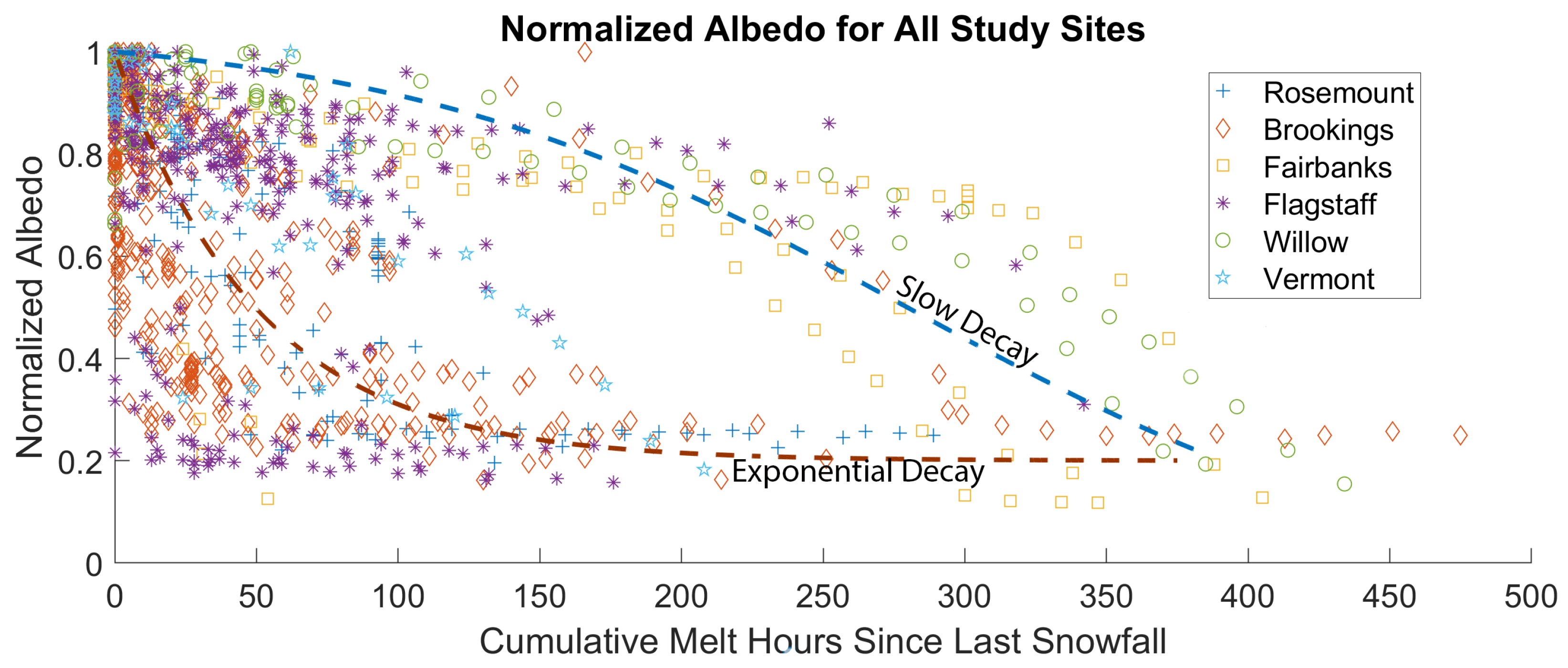
Once the data-cleaning process was completed, we plotted the normalized albedo data for all snow events with cumulative melt hour totals greater than zero for the six sites, as shown in Figure 7. The data in Figure 7 indicate two separate modes of albedo reduction: one in which the albedo declines quickly and levels off, and one in which the albedo declines slowly at first then rapidly declines with additional melt-hour accumulation.
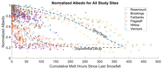
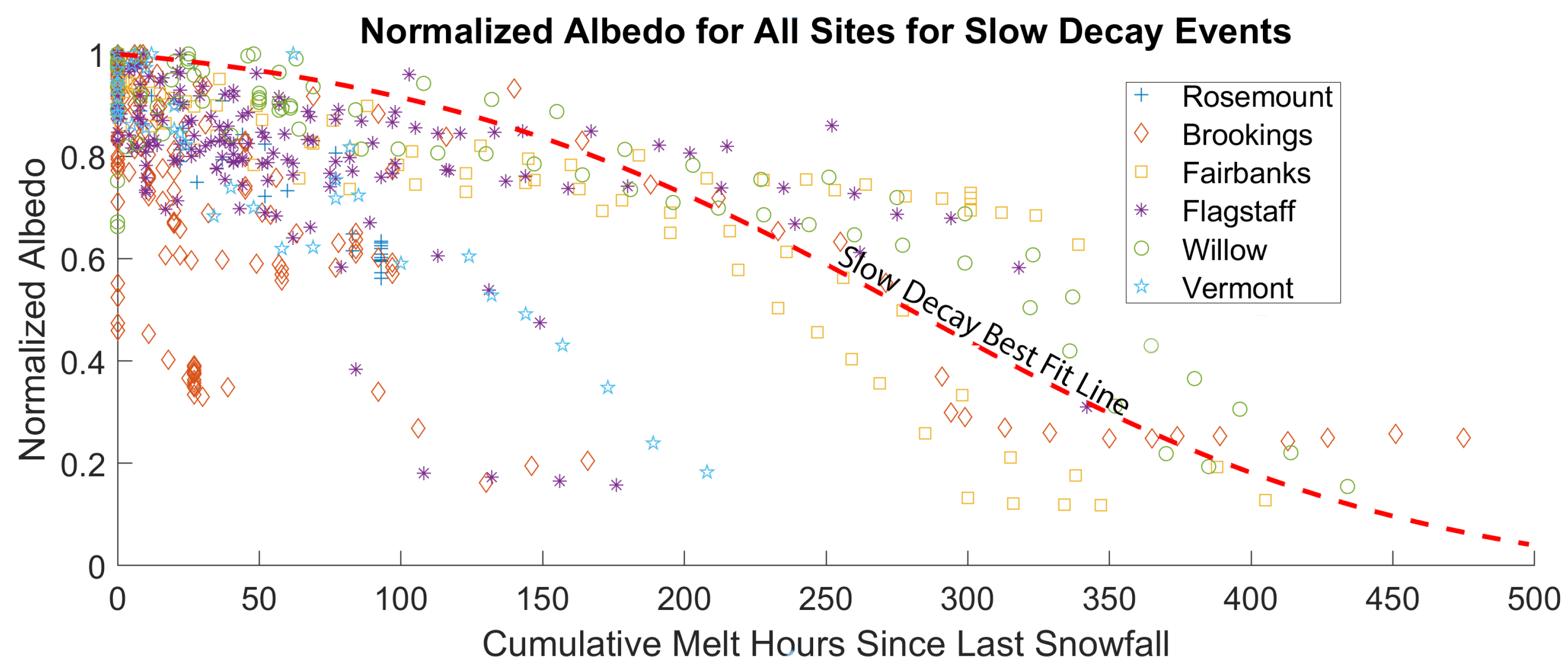
Figure 7.
Normalized albedo for all events from all study sites, graphed together along with modeled lines to highlight the two different albedo change modes that emerge from the data. The “slow decay” shape generally occurs in cases where the snow depth was greater than 10 cm in all of the preceding three days before the snow event began. The “exponential decay” shape generally occurs in cases where the snow depth was less than or equal to 10 cm on any of the preceding 3 days before the snow event began.
By grouping the events according to the shape of their albedo reduction, we were able to determine that the presence of snow prior to a snow event had a high correlation with the shape of the event’s albedo loss. As shown in Figure 8, in cases where the depth of snow on the ground exceeded 10 cm in all of the 3 days preceding the snow event, the normalized albedo of the snow decreases slightly over the first 200 melt hours, then quickly degrades to a minimum around 0.2.
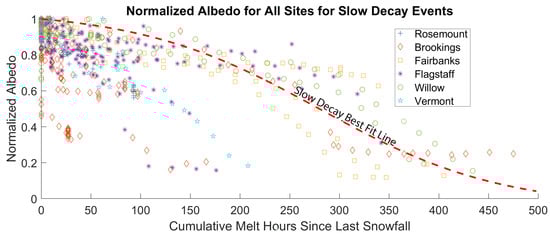
Figure 8.
The slow decay data graphed according to the melt hours to highlight the emerging curve shape that was used to develop the equations shown below.
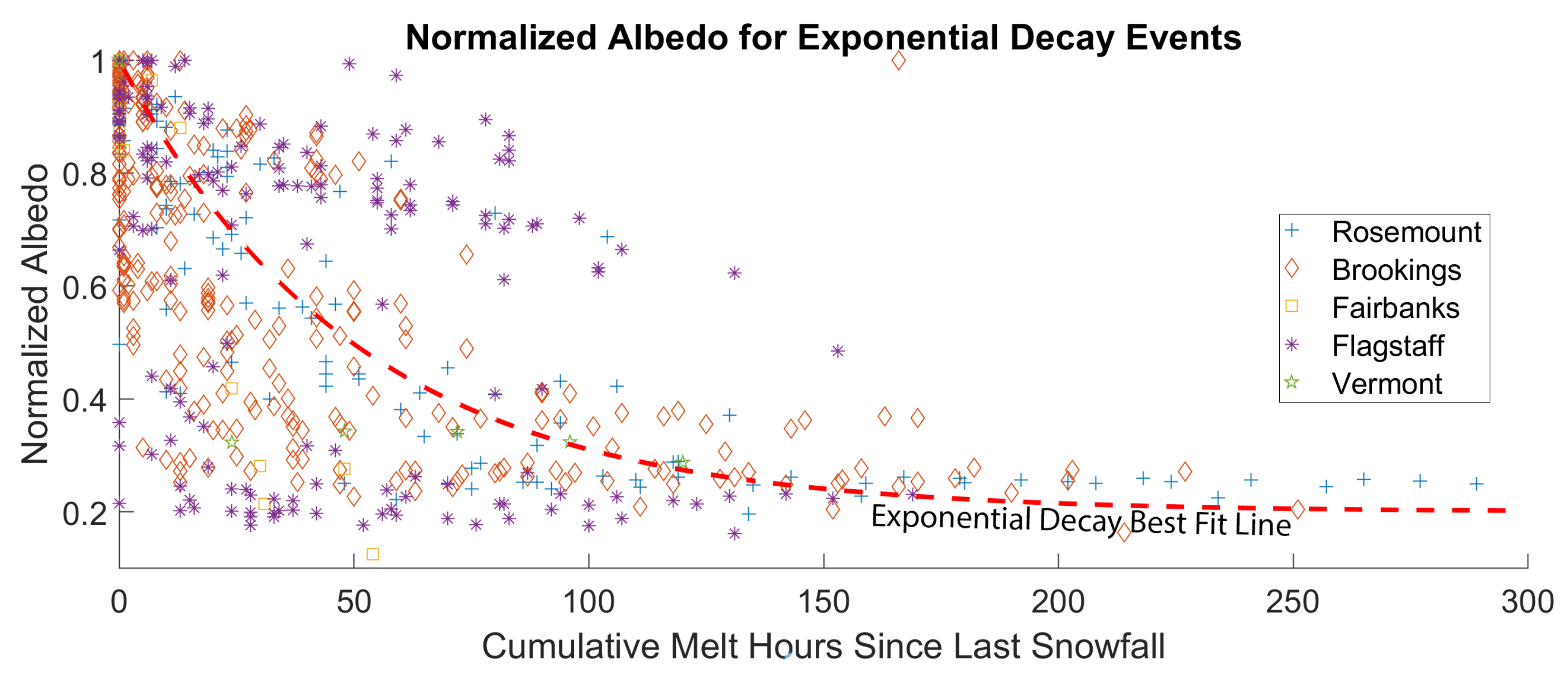
However, in cases where the snow depth was less than 10 cm in any of the 3 days preceding a snow event, the normalized albedo quickly decays to a minimum value also around 0.2, as shown in Figure 9. We have thus identified these two modes as the “exponential decay” mode, where there is little snow on the ground prior to a snowfall event, and the “slow decay” mode, where there is more snow on the ground prior to a snowfall event. The 10 cm snow depth was chosen because this snow depth appeared to be most effective in splitting the data into the two albedo change modes described above.
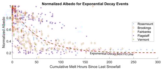
Figure 9.
The exponential decay data graphed according to the melt hours to highlight the emerging curve shape that was used to develop the equations shown below.
We acknowledge the presence of a middle decay population between the slow decay and exponential decay groups that is composed primarily of Flagstaff and Vermont data. Since these data appear in both decay shape datasets in Figure 8 and Figure 9, we believe that these snow events have snow depths in the prior 3 days that are close to the 10 cm division that would change their classification from one decay shape to another. The model in its present form accounts for the majority of observations.
We believe that this bifurcated albedo change is the result of snow melting to reveal patches of uncovered ground, which occurs more quickly when there is very little snow on the ground prior to a new snow event. The condition of low snow depth prior to a snowfall event is most common at the beginning of the snow season.
Based on the graph shown of the slow decay and exponential decay data in Figure 7, equations of the best-fit lines for the slow decay and exponential decay normalized albedo are as follows:
where
is the slow decay normalized albedo;
is the exponential decay normalized albedo;
M is the accumulated melt hours since the most recent snowfall.
The exponential decay curve has a natural minimum of 0.2, which is approximately the albedo of the underlying surfaces at the test sites. For other sites, i.e., those with higher or lower ground albedo, the function can be altered to accommodate the higher or lower ground albedo by changing the first term in the sum.
These equations were used as the basis for the melt-hour albedo model presented here. As explained above, the only two required inputs are temperature and snow depth. Model accuracy, however, can be improved if actual data for a specific site are available to replace the default data provided below. The optional inputs, where default data can be replaced with measured data, include the following:
- the albedo of the snow-free ground (default = 0.2);
- the snow depth before the first time step of the dataset (default = 0 cm);
- the minimum albedo present when snow is present (default = 0.4);
- the albedo of fresh snow for the site (default = 0.8);
- the minimum snow depth threshold used to indicate whether the modeled snow albedo or the ground albedo shall be used (default = 2.5 cm);
- the change in daily snow depth needed to trigger a snow event that resets the melt-hour count (default = 0 cm).
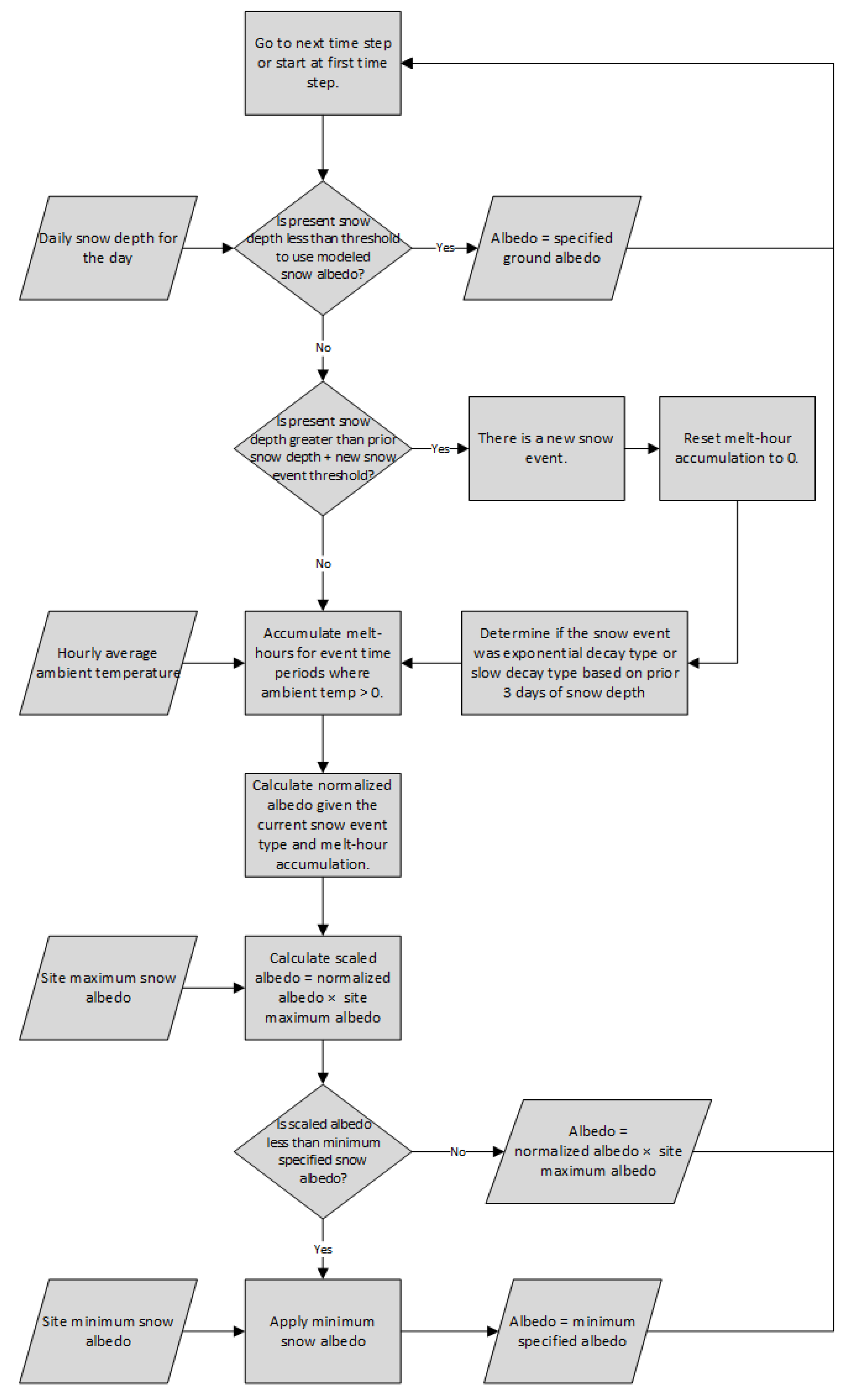
The melt-hour model works sequentially over time-series data, as shown in Figure 10. The model checks to see if the snow depth has increased since the last day of snow data. If the snow depth has increased, it is assumed that new snow has fallen and the melt-hour counter is set to 0. The model also determines if the snow event warrants albedo decay according to the exponential decay function or the slow decay function based on the snow depth values of the prior 3 days. If the total snow depth is less than 10 cm in any of the previous 3 days, then the exponential decay function is used; otherwise, the slow decay function is used. The model then begins stepping through the hourly time-series data and accumulating melt hours for any time period when the average hourly ambient temperature is greater than 0 °C. For each time step, the following tasks are executed:

Figure 10.
Flow chart of the advanced albedo model showing the model’s logic.
- Actual albedo is calculated as the product of the normalized albedo and the specified maximum albedo for the site as in Equation (3).
- If the calculated actual albedo values fall below the specified minimum albedo for the site, it is set to the minimum site albedo.
The model-calculated albedo is given by Equation (3):
where
is the albedo of the snow at a given time as calculated by the model;
is the normalized albedo, which may either be or depending on the snow conditions before the most recent snowfall;
is the albedo of freshly fallen snow for the site, an optional input to the model;
is the minimum albedo for the site, which is also an optional input to the model.
5. Results and Discussion
5.1. Validation against Measured Albedo
To validate the model, we collected temperature, albedo, and snow depth data from the following four geographically diverse sites during the winter of 2021–2022:
- Fairbanks, Alaska;
- Haines, Alaska;
- Calumet, Michigan;
- Fairlee, Vermont.
Validation data were collected identically to how the training data were collected using the process described earlier, and snow depth data were collected from the nearest location available from the NOAA National Climate Data Center database.
The temperature and snow depth data were used to model snow albedo, and the modeled albedo was compared with the measured albedo. The albedo estimated by the melt-hour model and the measured albedo were compared to assess the performance of the melt-hour albedo model and compare it with the performance of a traditional binary model which uses a fixed 0.8 albedo for snow and a fixed 0.2 albedo for snow-free conditions. The statistical validation results for the melt-hour albedo model are shown in Table 2 and Table 3.
Table 2.
Statistical comparisons using the measured training data against the traditional albedo assumptions and the melt-hour model data.
Table 3.
Statistical comparison using the validation data against the albedo change model data results and the traditional albedo assumptions.
The melt-hour albedo model dataset and the traditionally modeled dataset were compared to the measured validation dataset using the root-mean-square error (RMSE) method and the mean absolute percentage error (MAPE) method. This comparison revealed that the melt-hour albedo model does a better job than the traditional model at predicting the albedo at each location, as shown in Table 2 and Table 3.
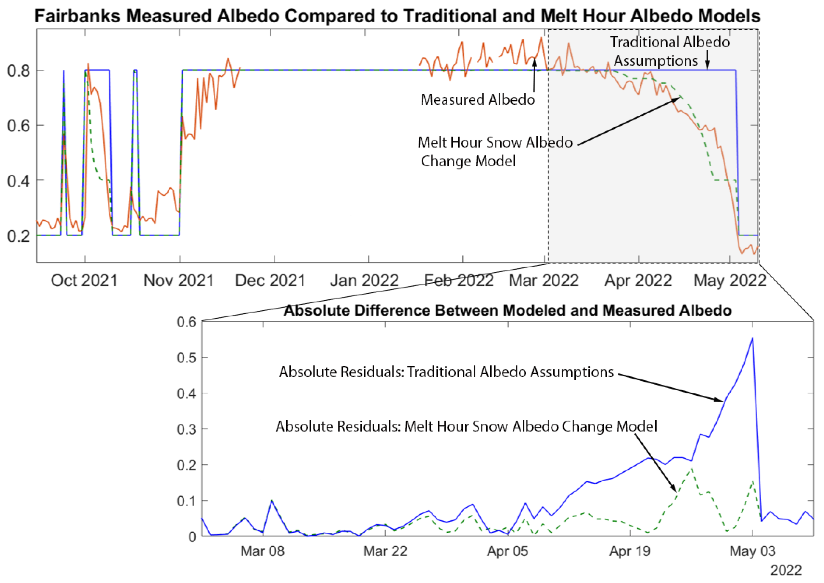
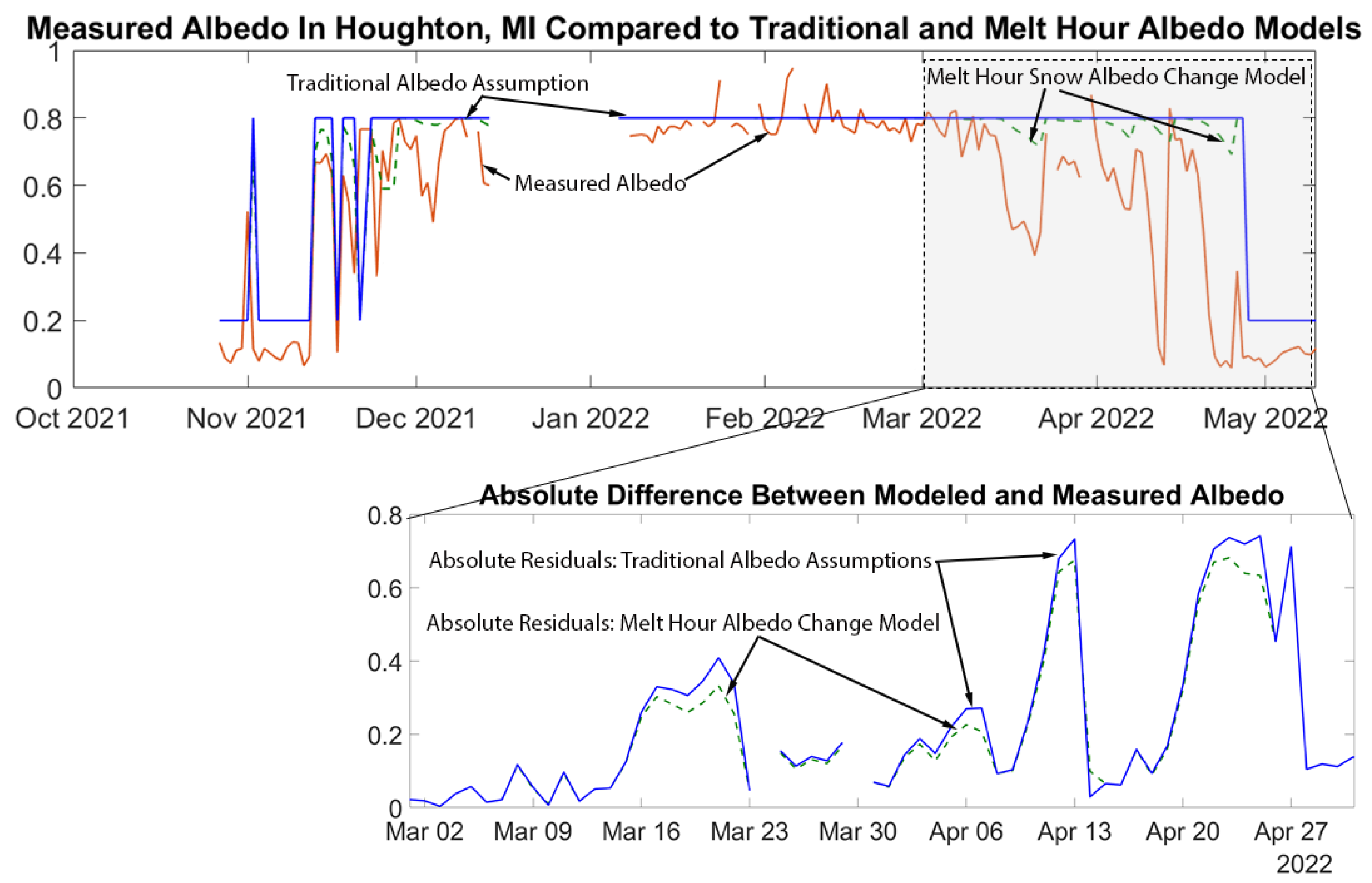
In addition to this statistical comparison, graphs of the measured albedo along with the modeled albedo derived from the melt-hour albedo model and the traditional model are shown in Figure 11 and Figure 12 below. The modeled albedo data are compared to the actual albedo data for Fairbanks, Alaska, and Houghton, Michigan, respectively. We suspect that the time periods where the measured and modeled albedo differ significantly in Figure 11 and Figure 12 are likely because the snow depth data that informs the modeled output were collected in these cases at a slightly different location than the albedometer location that was used for the validation dataset. For example, different wind patterns could cause snow to drift or be blown away at one location but not at the other location. Under this scenario, the underlying ground could be exposed at one location but not at the other. This is especially notable in Figure 12.
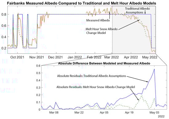
Figure 11.
Measured albedo from the Fairbanks (AK) validation dataset compared with the melt-hour albedo model data and the traditional model assumptions.
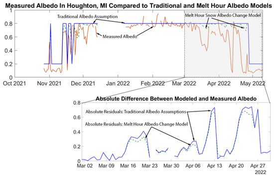
Figure 12.
Measured albedo from the Houghton (MI) validation dataset compared with the melt-hour albedo model data and the traditional model assumptions.
The melt-hour albedo model and the traditional model perform similarly when the time between snow events is short and/or when the hourly temperatures are regularly below 0 °C, as seen for January and February in both Figure 11 and Figure 12. When the time interval between snow events is longer and the daytime temperatures exceed 0 °C, the melt-hour albedo model performs better than the traditional model in estimating the snow albedo. The relative frequency of these conditions is likely location-dependent. For example, these conditions (longer periods between snow events and temperatures above freezing) may occur frequently in some locations throughout the entire winter, while other locations may see these conditions predominantly in the early and late periods of the snow season.
5.2. Validation against Satellite-Derived Albedo
Additional validation was completed to compare the results of the melt-hour albedo model with another commonly used source for ground albedo in PV applications, the National Solar Radiation Database (NSRDB) [34,35]. The NSRDB obtains ground albedo data from the Interactive Multisensor Snow and Ice Mapping System (IMS) [36]. Satellite networks such as the Polar and Geostationary Operational Environmental Satellite programs (POES/GOES) provide the data for the IMS and subsequently the NSRDB.
As the data generated from the NSRDB are based on satellite imagery, they do represent measurements that are directly informed by the albedo of the snow on the ground albeit through remote sensing methods rather than local measurements. Additionally, the NSRDB accounts for warmer temperatures in ice and snow by reducing the albedo when water is assumed to be on top of the surface [37]. Here, we compare the performance of the melt-hour model in predicting albedo with the performance of these remote sensing methods. However, we note that there are significant differences between the melt-hour model and the remote sensing options. First, as previously mentioned, remote sensing methods generate their estimates from energy reflected from the ground, while the melt-hour model attempts to estimate albedo without direct measurement of the surface based on historical changes in snow albedo due to time and temperature. Second, remote sensing methods have relatively low spatial resolution (currently either 4 km or 2 km) and are currently only available at latitudes less than 60°, whereas our model can be operated at a very local scale and wherever snow depth and temperature measurements are available. Third, while the NSRDB explicitly reduces the albedo of ice and snow at higher temperatures due to water accumulation, the melt-hour model only implicitly reduces the albedo to the extent that liquid water is accumulated on the surfaces under the measurement equipment. Finally, the NSRDB has a significant time lag between the measurement time and the release of the estimated surface albedo. The current time lag between an albedo measurement and its inclusion in the NSRDB is between 6 and 18 months (e.g., 2023 data are released in July 2024). This lag limits the use of the NSRDB for historical analyses, meaning that it cannot be used in real-time or hypothetical analyses.
In Table 4, we compare the errors of the melt-hour model with the NSRDB-reported ground albedo in Calumet, Michigan, and Fairlee, Vermont. Other locations found in our earlier validation dataset are above a 60° latitude and could not be included in this comparison due to the lack of NSRDB data at these sites. For this validation, we selected only the portion of winter with snow on the ground, in order to perform a fair comparison. The inclusion of only snow periods, rather than the entire winter season, accounts for the differences in performance between Table 3 and Table 4. As shown, the NSRDB albedo does report slightly lower RMSE and MAPE values than the melt-hour model, although both models performed better than a simple traditional 0.8/0.2 model (not shown).
Table 4.
Statistical comparisons of the albedo error for the melt-hour albedo model and the NSRDB, using Michigan data from between 15 November 2021 and 20 April 2022 and Vermont data from between 19 December 2021 and 15 March 2022.
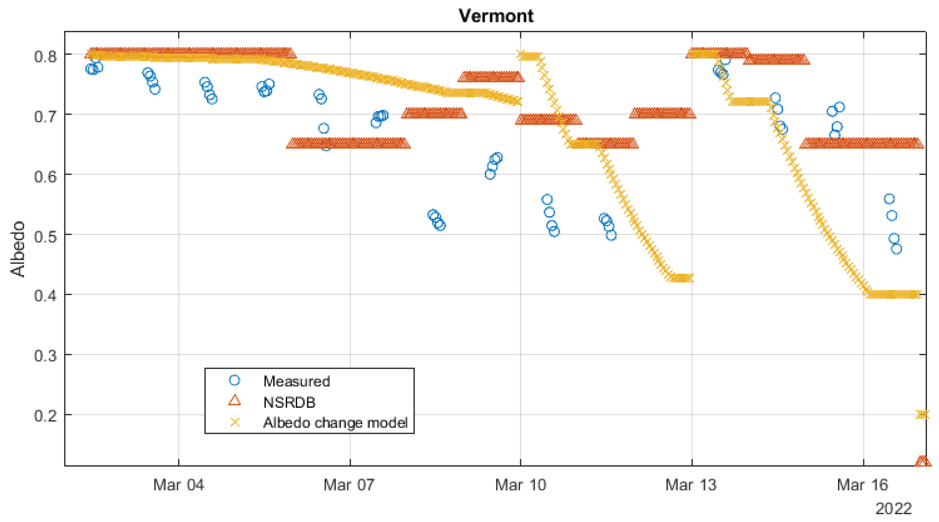
We present a portion of the time series for the Fairlee (VT) location with the measured albedo, the ground albedo from the NSRDB, and the albedo from the melt-hour model for March 2022 in Figure 13.
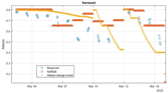
Figure 13.
Comparison of the measured albedo in Fairlee (VT) with the reported NSRDB ground albedo and the albedo as modeled using the melt-hour model.
5.3. Model Impact
To further examine the potential impact of the melt-hour albedo model on simulated PV system performance, POA irradiance data were generated using NREL’s System Advisor Model (SAM) for the Fairbanks site using three different albedo inputs. The albedo input was either (1) measured albedo from the Fairbanks test site, (2) modeled albedo using the traditional albedo model of 0.2 for non-snow conditions and 0.8 for snow conditions, or (3) albedo data from the melt-hour albedo model presented here. The additional required input data fields for the SAM include wind speed, wind direction, ambient temperature, relative humidity, and barometric pressure, as well as global (GHI) and diffuse (DHI) irradiance data, which were collected from the University of Alaska Fairbanks’s Solar Test Site on an averaged hourly basis. Beam irradiance (DNI) was calculated from the measured global and diffuse components using the following equation:
where z is the solar zenith angle.
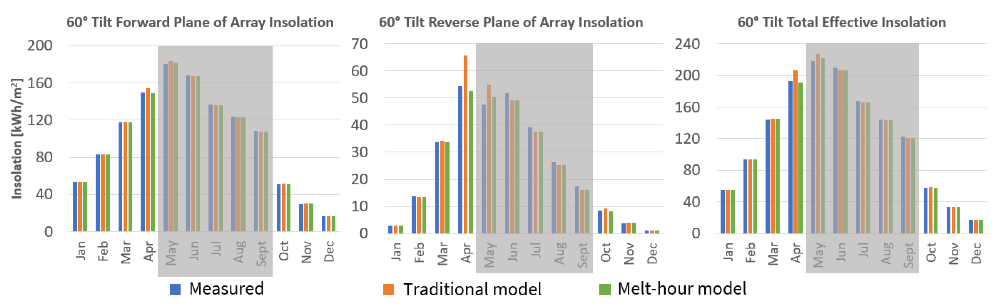
Three datasets that varied only in their albedo data were compiled and used to generate three SAMs using an array tilt of 60 degrees, which is the same tilt angle as that used in the Fairbanks test site modules where irradiance data were collected. Figure 14 presents the SAM-generated forward-facing and reverse-facing POA data, as well as total effective irradiance values created by summing the modeled forward-facing POA with the reverse-facing POA scaled by an assumed bifaciality factor of 0.8. The sum of the forward and scaled reverse irradiance is presented to estimate the available effective irradiance for a bifacial PV module with a 0.8 bifaciality factor.
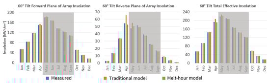
Figure 14.
SAM results for Fairbanks, Alaska (2022), showing forward, rear, and total effective POA insolation per month for a simulated array at a 60-degree tilt angle calculated using albedo from on-site measurements, a traditional binary model, and the melt-hour model. Gray regions indicate periods without snow cover.
Figure 14 shows that the irradiance simulation obtained using albedo data generated via the melt-hour albedo model is closer to that obtained using measured albedo during periods of the year with significant melt hours (such as April and October in this case), where the traditional albedo assumption of 0.8 was a significant overestimation. The difference is most apparent in the reverse POA data but is observable in the forward POA as well, as shown in Table 5, where the results are presented for the months with snow and show that the simulation using the albedo data generated with the melt-hour albedo model is closer to the measured albedo irradiance simulation than the traditional snow albedo assumptions.
Table 5.
Percent and absolute errors for rear POA and front POA modeled in the SAM using measured albedo, melt-hour model albedo, and traditional binary model albedo data for the months with significant snow cover shown in Figure 14.
6. Conclusions
As bifacial PV systems proliferate across high-latitude locations, where snowfall predictably occurs, accurate albedo projections will increasingly factor into PV performance models. In this paper, we have presented a model for predicting snow albedo when time-series temperature and snow depth data are known. This model has several advantages:
- It uses commonly available ambient temperature and snow depth data;
- It allows users the ability to incorporate site-specific measured data to replace default values and improve model accuracy;
- It is available in pvlib model repositories [38];
- It allows for real-time estimation of snow surface albedo.
However, the model is unable to account for:
- Situations where snow depth may change independently of snowfall or temperature-driven melting, such as due to wind-blown snow or a rainfall event;
- Snow albedo changes that are not caused by time and temperature, such as soiling of the snow by particulates, including ash, dust, debris, etc.
We acknowledge there are other models, such as the energy-balance model described earlier, that might better predict snow albedo, but we believe that the additional data requirements of those models render them impractical for many PV modeling applications.
We have compared the performance of the proposed melt-hour albedo model to that of other simple performance models, such as the binary model that applies a high albedo when snow is present and a low albedo when snow is absent, and conclude that the melt-hour albedo model better estimates the albedo of snow at a site. We have also found that the melt-hour albedo model does not perform as well as the NSRDB albedo estimates. While we acknowledge that albedo estimates based on remote sensing data, such as those from the NSRDB, do compare very favorably with measured albedo, these remote-sensing-based estimates are typically available after a significant time lag, which makes them unsuitable for near-real-time applications. In addition, the NSRDB is not currently available for locations north of 60° latitude, despite the rapid growth of solar PV in these regions.
Supplementary Materials
The following supporting information can be downloaded at https://www.mdpi.com/article/10.3390/solar4030019/s1: Riley, D. High Irradiance Conditions; Sandia National Lab: Albuquerque, NM, USA. Upublished Report.
Author Contributions
Conceptualization, C.P. and D.R.; methodology, C.P. and D.R.; software, C.P. and D.R.; validation, C.P., D.R. and H.T.; formal analysis, C.P. and D.R.; investigation, C.P. and D.R.; resources, C.P., D.R. and L.B.; data curation, C.P. and D.R.; writing—original draft preparation, C.P. and D.R.; writing—review and editing, C.P., D.R., H.T. and L.B.; visualization, C.P., D.R. and H.T.; supervision, C.P. and L.B.; project administration, L.B. and C.P.; funding acquisition, L.B., C.P. and D.R. All authors have read and agreed to the published version of the manuscript.
Funding
This research is based upon work supported by the U.S. Department of Energy’s Office of Energy Efficiency and Renewable Energy (EERE) under the Solar Energy Technologies Office Award Number 38527.
Institutional Review Board Statement
Not applicable.
Informed Consent Statement
Not applicable.
Data Availability Statement
The original contributions presented in the study are included in the article and Supplementary Materials, further inquiries can be directed to the corresponding author. Data from the NSRDB may be accessed here: https://nsrdb.nrel.gov/ (accessed on 23 May 2024). The pvlib Python package can be found here: https://github.com/pvlib/pvlib-python (accessed on 3 April 2024).
Conflicts of Interest
The authors declare no conflicts of interest.
Abbreviations
The following abbreviations are used in this manuscript:
| GHI | global horizontal irradiance |
| DHI | diffuse horizontal irradiance |
| DNI | direct normal irradiance |
| RHI | reflected horizontal irradiance |
| SAM | System Advisor Model |
| NSRDB | National Solar Radiation Database |
| RMSE | root-mean-square error |
| MAPE | mean absolute percentage error |
| NREL | National Renewable Energy Laboratory |
| PV | photovoltaic(s) |
| ITRPV | International Technology Roadmap for Photovoltaic |
| LCOE | levelized cost of energy |
| POA | plane-of-array |
| NOAA | National Oceanic and Atmospheric Administration |
| MISR | Multi-Angle Imaging Spectroradiometer |
| AVHRR | Advanced Very High Resolution Radiometer |
| MODIS | Moderate Resolution Imaging Spectroradiometer |
References
- Burnham, L. PV Performance and Reliability in Snowy Climates: Opportunities and Challenges; Technical Report; Sandia National Lab. (SNL-NM): Albuquerque, NM, USA, 2019. [Google Scholar]
- Burnham, L.; Riley, D.; Walker, B.; Pearce, J.M. Performance of bifacial photovoltaic modules on a dual-axis tracker in a high-latitude, high-albedo environment. In Proceedings of the 2019 IEEE 46th Photovoltaic Specialists Conference (PVSC), Chicago, IL, USA, 16–21 June 2019; pp. 1320–1327. [Google Scholar]
- Rodríguez-Gallegos, C.D.; Liu, H.; Gandhi, O.; Singh, J.P.; Krishnamurthy, V.; Kumar, A.; Stein, J.S.; Wang, S.; Li, L.; Reindl, T.; et al. Global techno-economic performance of bifacial and tracking photovoltaic systems. Joule 2020, 4, 1514–1541. [Google Scholar] [CrossRef]
- Deline, C.; Ayala Pelaez, S.; MacAlpine, S.; Olalla, C. Estimating and parameterizing mismatch power loss in bifacial photovoltaic systems. Prog. Photovoltaics Res. Appl. 2020, 28, 691–703. [Google Scholar] [CrossRef]
- Stein, J.; Reise, C.; Castro, J.B.; Friesen, G.; Maugeri, G.; Urrejola, E.; Ranta, S. Bifacial Photovoltaic Modules and Systems: Experience and Results from International Research and Pilot Applications; Technical Report; Sandia National Lab. (SNL-NM): Albuquerque, NM, USA; Fraunhofer ISE: Freiburg, Germany, 2021. [Google Scholar]
- Pike, C.; Whitney, E.; Wilber, M.; Stein, J.S. Field performance of south-facing and east-west facing bifacial modules in the arctic. Energies 2021, 14, 1210. [Google Scholar] [CrossRef]
- DeMarban, A. Developers Set to Flip Switch at Alaska’s Largest Solar Farm. Anchorage Daily News, 31 August 2023; pp. A1, A15. [Google Scholar]
- Baliozian, P.; Tepner, S.; Fischer, M.; Trube, J.; Herritsch, S.; Gensowski, K.; Clement, F.; Nold, S.; Preu, R. The international technology roadmap for photovoltaics and the significance of its decade-long projections. In Proceedings of the 37th European PV Solar Energy Conference and Exhibition, Online, 7–11 September 2020; Volume 7, p. 11. [Google Scholar]
- Marion, B. Measured and satellite-derived albedo data for estimating bifacial photovoltaic system performance. Sol. Energy 2021, 215, 321–327. [Google Scholar] [CrossRef]
- Chiodetti, M.; Kang, J.; Reise, C.; Lindsay, A. Predicting yields of bifacial PV power plants—What accuracy is possible? System 2018, 2, 1–7. [Google Scholar]
- Kotak, Y.; Gul, M.; Muneer, T.; Ivanova, S. Investigating the impact of ground albedo on the performance of PV systems. In Proceedings of the CIBSE Technical Symposium, London, UK, 16–17 April 2015. [Google Scholar]
- PVsyst. Albedo Coefficient, PVsyst 7 Help Documentation. Available online: https://www.pvsyst.com/help/albedo.htm (accessed on 20 June 2024).
- Sandia National Laboratory; PV Performance Modeling Collaborative. Albedo. Available online: https://pvpmc.sandia.gov/modeling-guide/1-weather-design-inputs/plane-of-array-poa-irradiance/calculating-poa-irradiance/poa-ground-reflected/albedo/ (accessed on 20 June 2024).
- Kane, D.L.; Gieck, R.E.; Hinzman, L.D. Snowmelt modeling at small Alaskan Arctic watershed. J. Hydrol. Eng. 1997, 2, 204–210. [Google Scholar] [CrossRef]
- Mueller-Stoffels, M.; Wackerbauer, R. Regular network model for the sea ice-albedo feedback in the Arctic. Chaos Interdiscip. J. Nonlinear Sci. 2011, 21, 013111. [Google Scholar] [CrossRef]
- Calleja, J.F.; Muñiz, R.; Fernández, S.; Corbea-Pérez, A.; Peón, J.; Otero, J.; Navarro, F. Snow albedo seasonal decay and its relation with shortwave radiation, surface temperature and topography over an Antarctic ice cap. IEEE J. Sel. Top. Appl. Earth Obs. Remote Sens. 2021, 14, 2162–2172. [Google Scholar] [CrossRef]
- Rango, A.; Martinec, J. Revisiting the degree-day method for snowmelt computations 1. JAWRA J. Am. Water Resour. Assoc. 1995, 31, 657–669. [Google Scholar] [CrossRef]
- Dirmhirn, I.; Eaton, F.D. Some characteristics of the albedo of snow. J. Appl. Meteorol. Climatol. 1975, 14, 375–379. [Google Scholar] [CrossRef]
- Anderson, E. Techniques for predicting snow cover runoff. In Role of Snow and Ice in Hydrology: Proceedings of the Banff Symposia; Unesco-WMO-IAHS: Geneva, Switzerland, 1972. [Google Scholar]
- Jin, Z.; Simpson, J.J. Anisotropic reflectance of snow observed from space over the Arctic and its effect on solar energy balance. Remote Sens. Environ. 2001, 75, 63–75. [Google Scholar] [CrossRef]
- Stroeve, J.C.; Nolin, A.W. New methods to infer snow albedo from the MISR instrument with applications to the Greenland ice sheet. IEEE Trans. Geosci. Remote Sens. 2002, 40, 1616–1625. [Google Scholar] [CrossRef]
- Amaral, T.; Wake, C.P.; Dibb, J.E.; Burakowski, E.A.; Stampone, M. A simple model of snow albedo decay using observations from the Community Collaborative Rain, Hail, and Snow-Albedo (CoCoRaHS-Albedo) Network. J. Glaciol. 2017, 63, 877–887. [Google Scholar] [CrossRef]
- Ameriflux. Ameriflux: Measuring Carbon, Water, and Energy Flux across the Americas. Available online: https://ameriflux.lbl.gov/ (accessed on 31 July 2024).
- Dore, S.; Kolb, T. AmeriFlux AmeriFlux US-Fwf Flagstaff-Wildfire; Lawrence Berkeley National Laboratory (LBNL): Berkeley, CA, USA; Northern Arizona University: Flagstaff, AZ, USA, 2016. [Google Scholar]
- Meyers, T. AmeriFlux AmeriFlux US-Bkg Brookings; Lawrence Berkeley National Laboratory (LBNL): Berkeley, CA, USA, 2016. [Google Scholar]
- Baker, J.; Griffis, T. AmeriFlux FLUXNET-1F US-Ro4 Rosemount Prairie; Lawrence Berkeley National Lab. (LBNL): Berkeley, CA, USA; University of Minnesota: Minneapolis, MN, USA; US Department of Agriculture (USDA): Washington, DC, USA, 2022. [Google Scholar]
- National Centers for Environmental Information (NCEI). Climate Data Online. Available online: https://www.ncdc.noaa.gov/cdo-web/ (accessed on 22 June 2021).
- Sengupta, M.; Habte, A.; Wilbert, S.; Gueymard, C.; Remund, J. Best Practices Handbook for the Collection and Use of Solar Resource Data for Solar Energy Applications, 3rd ed.; National Renewable Energy Laboratory: Golden, CO, USA, 2021. [Google Scholar] [CrossRef]
- Riley, D. High Irradiance Conditions; Sandia National Lab: Albuquerque, NM, USA, Upublished Report.
- de Vrese, P.; Stacke, T.; Caves Rugenstein, J.; Goodman, J.; Brovkin, V. Snowfall-albedo feedbacks could have led to deglaciation of snowball Earth starting from mid-latitudes. Commun. Earth Environ. 2021, 2, 91. [Google Scholar] [CrossRef]
- Markvart, T.; Castañer, L. Practical Handbook of Photovoltaics: Fundamentals and Applications; Elsevier: Amsterdam, The Netherlands, 2003. [Google Scholar]
- Maxwell, E.; Wilcox, S.; Rymes, M. Users Manual for SERI QC Software, Assessing the Quality of Solar Radiation Data; Solar Energy Research Institute: Golden, CO, USA, 1993. [Google Scholar]
- Song, J. Diurnal asymmetry in surface albedo. Agric. For. Meteorol. 1998, 92, 181–189. [Google Scholar] [CrossRef]
- National Renewable Energy Laboratory. NSRDB: National Solar Radiation Database. Available online: https://nsrdb.nrel.gov (accessed on 20 June 2024).
- Sengupta, M.; Xie, Y.; Lopez, A.; Habte, A.; Maclaurin, G.; Shelby, J. The national solar radiation data base (NSRDB). Renew. Sustain. Energy Rev. 2018, 89, 51–60. [Google Scholar] [CrossRef]
- U.S. National Ice Center. IMS Snow and Ice Products. Available online: https://usicecenter.gov/Products/ImsHome (accessed on 20 June 2024).
- Ross, B.; Walsh, J.E. A comparison of simulated and observed fluctuations in summertime Arctic surface albedo. J. Geophys. Res. Oceans 1987, 92, 13115–13125. [Google Scholar] [CrossRef]
- Holmgren, W.F.; Hansen, C.W.; Mikofski, M.A. pvlib python: A python package for modeling solar energy systems. J. Open Source Softw. 2018, 3, 884. [Google Scholar] [CrossRef]
Disclaimer/Publisher’s Note: The statements, opinions and data contained in all publications are solely those of the individual author(s) and contributor(s) and not of MDPI and/or the editor(s). MDPI and/or the editor(s) disclaim responsibility for any injury to people or property resulting from any ideas, methods, instructions or products referred to in the content. |
© 2024 by the authors. Licensee MDPI, Basel, Switzerland. This article is an open access article distributed under the terms and conditions of the Creative Commons Attribution (CC BY) license (https://creativecommons.org/licenses/by/4.0/).