LCA of Soybean Supply Chain Produced in the State of Pará, Located in the Brazilian Amazon Biome ^†

Abstract

Recently, Brazil became the biggest soybean producer and exporter in the world. The state of Pará, located in the Brazilian amazon biome, became one of the last agricultural frontiers of the country, which positively increased the soybean cultivation along it is territory. However, it is necessary to know the associated environmental impacts along the supply chain. Thus, we are applying the life cycle assessment (LCA) methodology using openLCA software to two producing regions: northeast pole (Paragominas) and south pole (Redenção). Based on the cradle to grave scope, the Recipe Midpoint (H) and Intergovernmental Panel on Climate Change (IPCC) methods of the environmental impact categories were used. To calculate the land use change (LUC), we used the BRLUC regionalized model (v1.3). The obtained results showed that LUC was mainly responsible for the global warming potential (GWP) along all soybean supply chains, especially when land occupied with tropical forests was adapted for growing soybeans. Despite the largest distance between the origin and destiny (road + railway = 1306 km), the soybean produced in the south pole (Redenção) is better shipped through the TEGRAM port of São Luis–Maranhão due to the use of multimodal platforms (lorry + train), allowing for a more efficient logistical performance (greater loads of grains transported and less environmental impact). The soybean produced in northeast pole (Paragominas) is better shipped through the ports around Barcarena–Pará due to the short distance by road (average 350 km) and hence less environment impact.

1. Introduction

In the last decades, soybean production has increased due to its use as an important source of protein and oil, which has been stimulated by the growing demand for feed, food, and other by-products consumed worldwide [1]. Throughout 2019/2020, the USDA estimated a harvest of 122.63 million hectares destined for soybean worldwide, corresponding to a production of around 339 million tonnes [2].

Three countries (Brazil, USA, and Argentina) are responsible for approximately 80.8% of all soybeans produced in the world. Among them, Brazil appears to be the main soybean player in the world, as it has the largest cultivated area (36.9 million hectares), largest production (128.5 million tonnes), and is the largest exporter [2].

Located in the north of Brazil, the state of Pará is a new agricultural frontier in the country. In the 2019/2020 harvest, 1859 million tonnes of grain were produced in an area of 607.4 thousand hectares for soybean cultivation. Pará has three producing regions, with the Paragominas pole and its municipalities being the largest producer region with 339.5 thousand hectares. In the south of the state, the Redenção pole has consists of 25% of soy production. The region of Baixo Amazonas (Santarém pole), in the west of the state, produces the remaining amount [3,4].

In 2006, under pressure from global retailers and non-governmental organizations (NGOs), the Brazilian Soy Moratorium (SoyM) was instituted in Brazil with the aim of achieving zero deforestation in the Amazon rainforest associated with soybean agriculture [5]. Thus, the soybean cultivated in recently deforested amazon biome areas will not be marketed with the signatory trading’s companies of agreement.

Agricultural activities are linked to greenhouse gas (GHG) emissions. Thus, the increasing food production trends associated with global population growth, need to be evaluated frequently in order to discover the GHG emissions of crops [6]. However, other impact categories should also be monitored, such as human toxicity, freshwater toxicity, freshwater eutrophication, and terrestrial acidification in soybean and sunflower cultivation [7].

Thus, life cycle assessment (LCA) is an important tool that allows for quantifying the environmental impact throughout all stages of the supply chain. It can be considered from the raw material used along the production chain to the applied process (recycling or disposal) at the end of the product’s life [8].

In LCA studies, we consider two types of scopes: cradle-to-gate or cradle-to-grave, for a broader approach. Consequently, topics such as GHG emissions associated with the production of 1 kg of soybeans with a cradle-to-gate scope can be addressed [9], as well as quantifying the environmental impacts on the production of 1 kg of soybeans or 1 L of biodiesel involving the cradle-to-grave scope [10].

Here, we cover all stages of soybean cultivation and inputs used. However, outside the scope of the cradle-to-farm, we also consider the transportation phase. This considers which type of modal most affects the environment, and also analyzes the distances from the site of production origin to the port of shipment. Thus, for those who are interested in the subject, we seek to describe the main hotspots of soybean supply chain in each category of environmental, with reference to two poles (Paragominas and Redenção) in the state of Pará, Brazil, using LCA methodology.

2. Materials and Methods

2.1. Study Area and Crops

This study was based on the non-irrigated soybean (Glycine max (L.) Merrill) cultivation system in two production regions (pole): the northeast pole (Paragominas) and the south pole (Redenção) in the state of Pará, Brazil. The average annual rainfall of the regions is 1700 mm and 2000 mm, respectively, per year [11].

2.2. Life Cycle Assessment Methodology

This LCA approach follows the principles and framework [8], and requirements and guidelines [12] of the International Standards Organization. The LCA method is appropriate to quantify the level of environmental impacts associated with the activities, by identifying the main hotspots involved in each phase along the soybean supply chain. These results can serve as guidelines, helping towards more environmentally friendly decisions forward so as to minimize more impactful activities on the environment.

2.2.1. Aim of the Study

The focus of this study is to quantify the environmental impacts associated with the soybean supply chain in two production hubs in the state of Pará, Brazil, using LCA methodology. In addition, we seek to find which is the best destination (port of shipment) for the flow of harvested grains, considering the travel distances (

Table 1. Traveling distances (km), transportation modals, and port of shipment.

Pole Origin	Road Distance (km)	Multimodal Platform	Railway Distance (km)	Total Distance Traveled (km)	Port of Shipment
Paragominas (PGM)	351			351	BAR-PA 3
Paragominas (PGM)	406	Porto Franco-MA 1	783	1189	SLZ-MA 4
Redenção (RDX)	827			827	BAR-PA 3
Redenção (RDX)	305	Palmeirante-TO 2	1001	1306	SLZ-MA 4

¹ Transshipment in Porto Franco, state of Maranhão; ² Transshipment in Palmeirante, state of Tocantins; ³ Barcarena, state of Pará; ⁴ São Luis, state of Maranhão.

) and the type of transportation modals involved.

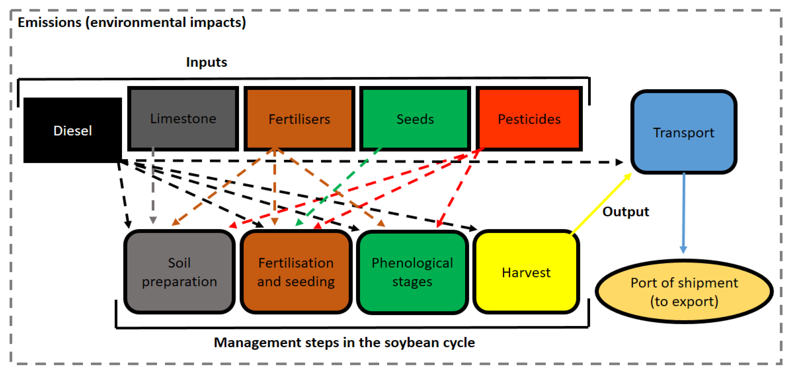
2.2.2. Scope of the Study and Crop Management

We applied a cradle-to-grave scope, without considering the stages of drying and warehousing grains, as well as the final consumption by customers. After the farm gate, only the transportation of harvested grains from the farm to the two shipment ports was considered: port of Barcarena, in the state of Pará and port TEGRAM, Grains Terminal of Maranhão (acronym in Portuguese), located in São Luis do Maranhão. Our functional unit (FU) was 1 kg of soybean. In the agricultural phase, the input flows (production factors) were approached (Figure 1).

Commonly in the region, NPK chemical fertilizers are used in sowing. However, as potassium is a salt, fertilizing should not exceed 70 kg K₂O ha⁻¹ so as to minimize the risks of stress on crop development, hence affecting the uniformity of the population and their yield. Thus, if necessary and according to the soil analysis, a complement of K₂O fertilizer using a broadcaster a few weeks before sowing or 30 days after sowing should be done. This procedure also aims to avoid losses of K₂O for leaching, mainly in sandy texture soils.

It is known that soybean is a Fabaceae family plant capable of converting gaseous nitrogen from the atmosphere into NH₄⁺ through a symbiotic relationship with N-fixing bacteria. Therefore, all farmers inoculate Bradyrhizobium japonicum in seeds before sowing. However, the impact of inoculation was not considered in our inventory. A little bit of chemical nitrogen is used in the NPK formulation (7 kg N·ha⁻¹) so as to favor the initial growth of the plants. Generally, tropical soils are low in phosphorus. Thereby, for soybean management, the amount used is in the region of 100 to 125 kg of P₂O₅·ha⁻¹.

In relation to spraying along the crop cycle, usually four fungicides, two insecticides, and one to three herbicides (pre and post-emergent) were applied against diseases, pests, and for cleaning weeds in the crop field, respectively. These operations correspond to a range of seven to nine pesticide applications.

2.2.3. Software, Database and LCIA Method Used

OpenLCA software was used for information processing. Input and output flows of the process were extracted from the French Life Cycle Inventory (LCI) database Agribalyse (v.3). We used the average inventory values from four farms, and two life cycle impact assessment (LCIA) methods were applied—Recipe Midpoint (H) and IPCC 2013.

2.2.4. Land Use Change (LUC)

To calculate the LUC, we used the BRLUC regionalized model (v1.3) of [13], considering a 20 years temporal coverage (1999–2018) associated with the expansion of the planted area and other soil uses in Pará state. The model considered the influence of possible transitions in different land uses, estimating three emission scenarios: (I) minimum, (II) maximum, and (III) proportional rate. To estimate scenarios (I) and (II), BRLUC considered the allocation of areas and emission rates using the simplex method based on a linear programming problem.

3. Results

Table 2. Input and output of soybean production systems in the state of Pará, Brazil (FU 1 kg of soybean).

Input	Amount	Output	Amount
Application of plant protection product, by field sprayer	0.00258 ha	Ammonia (NH3)	0.00028 kg
Combine harvesting	0.00030 ha	Dinitrogen monoxide (N2O)	0.00063 kg
Fertilizing, by broadcaster	0.00030 ha	Nitrate	0.02804 kg
Sowing	0.00030 ha	Nitrogen oxides	0.00013 kg
Tillage, harrowing, by spring tine harrow	0.00028 ha	Carbon dioxide, fossil	0.02502 kg
Tillage, ploughing	0.00010 ha	2,4-D	0.00045 kg
Transport, tractor and trailer, agricultural	0.01570 t km	Acetamiprid	2.65000 × 10−5 kg
Soybean seed, for sowing	0.01280 kg	Fenpropathrin	1.70000 × 10−5 kg
Lime	0.04929 kg	Fluazinam	0.00011 kg
Urea, as N	0.00212 kg	Glyphosate	0.00061 kg
Phosphate fertilizer, as P2O5	0.03576 kg	Mancozeb	0.00034 kg
Phosphate Rock, as P2O5, beneficiated, dry	0.00212 kg	Prothioconazol	2.65000 × 10−5 kg
Potassium chloride, as K2O	0.03030 kg	Pyraclostrobin (prop)	2.52300 × 10−5 kg
Occupation, annual crop, non-irrigated, intensive	3.25298 m2 year	Pyriproxyfen	7.60000 × 10−6 kg
Transformation, from annual crop, non-irrigated	3.03030 m2	Phosphorus	0.00128 kg
Transformation, to annual crop, non-irrigated, intensive	3.03030 m2	Thiophanate-methyl	0.00011 kg
Energy, gross calorific value, in biomass	20.5000 MJ	Trifloxystrobin	2.27000 × 10−5 kg
Carbon dioxide, in air	1.37808 kg	Soybean production	1 kg
2,4-dichlorophenol	0.00045 kg
Pesticide, unspecified	7.44300 × 10−5 kg
Pyrethroid-compound	1.70000 × 10−5 kg
Pyridine-compound	0.00012 kg
Glyphosate	0.00061 kg
Mancozeb	0.00034 kg
Triazine-compound	2.65000 × 10−5 kg
[Sulfonyl] urea-compound	0.00011 kg

describes the inventories (input and output flows) used for the soybean production process, standardized for the FU of 1 kg of soybean (fresh matter). It is worth mentioning that the nitrate output (NO₃⁻) was calculated according to [14]. This proposed model (SQCB-NO3) considers the interactions between the nitrogen inputs in fertilization and the nitrogen contained in organic matter in the soil, among other variables.

Table 3. Life cycle impact assessment (LCIA) results at recipe midpoint (H) (FU 1 kg of soybean).

Impact Category	Unit	Total Emissions	Main Hotspot
Agricultural land occupation (ALOP)	m2 year	3.25298 × 100	PS = 3.25298 × 100 (100%)
Climate change (GWP100)	kg CO2-Eq	0.48312 × 100	PS = 0.21154 × 100 (43.8%)
Freshwater ecotoxicity (FETPinf)	kg 1,4-DCB-Eq	1.99383 × 10−2	PS = 1.946 × 10−2 (95.4%)
Freshwater eutrophication (FEP)	kg P-Eq	1.89967 × 10−4	PS = 1.011 × 10−4 (53.2%)
Human toxicity (HTPinf)	kg 1,4-DCB-Eq	0.10915 × 100	MFPF = 4.81 × 10−2 (44.1%)
Ionising radiation (IRP_HE)	kg U235-Eq	1.97907 × 10−2	MFPF = 8.14 × 10−3 (41.1%)
Marine ecotoxicity (METPinf)	kg 1,4-DCB-Eq	2.42444 × 10−3	PS = 1.429 × 10−3 (58.9%)
Marine eutrophication (MEP)	kg N-Eq	7.10465 × 10−3	PS = 6.413 × 10−3 (90.2%)
Ozone depletion (ODPinf)	kg CFC-11-Eq	2.82500 × 108	MFCH = 7.59 × 10−9 (26.9%)
Particulate matter formation (PMFP)	kg PM10-Eq	9.67280 × 10−3	MFPF = 3.24 × 10−4 (29.6%)
Photochemical oxidant formation (POFP)	kg NMVOC-Eq	2.03110 × 10−3	MFCH = 6.67 × 10−3 (32.8%)
Terrestrial acidification (TAP100)	kg SO2-Eq	2.57782 × 10−3	PS = 7.623 × 10−4 (29.6%)
Terrestrial ecotoxicity (TETPinf)	kg 1,4-DCB-Eq	0.01326 × 100	PS = 1.243 × 10−2 (93.7%)

PS = production system; MFPF = market for phosphate fertilizer; MFCH = market for combine harvesting.

describes 13 impact categories other than the 18 presents in the Recipe Midpoint (H). These results do not support impacts from only five categories, which were not reported because the values were null.

All pesticides (active principle) used in field must be placed as the output of the production system (agricultural phase) in the category emissions to soil. Their chemical groups were placed as inputs. Ammonia, nitrogen oxides, dinitrogen monoxide, and carbon dioxide fossil emissions were calculated according to the guidelines in [15]. The yield of soybean in each site was 3300 kg·ha⁻¹, considering 115 days for the soybean cycle of cultivation.

In addition to the total values for each impact category considering the FU production process, the main hotspots (most impactful process in the category) were also highlighted, with the results and percentage contributing to the total impact category.

The soybeans produced in each production pole have two possible destination routes. Therefore, the CO₂ emissions per kg soy (fresh matter) along the routes were calculated. Both routes to the port of Barcarena involved lorry transport, while the routes to São Luis (TEGRAM) involved lorry and railway transport. Thus, the emissions from Paragominas to Barcarena were lower than to São Luis, while the converse was observed in Redenção, where the emissions to Barcarena were higher than to São Luis (Figure 2).

Table 4. LUC and estimated scenarios of CO2 emissions between 1999 and 2018 in the state of Pará.

Soybean Crop Expansion (%)	Scenarios	Emissions (tCO2 Eq·ha−1·yr−1)	T0 Soy (ha), Pre Existent 1999	T1 Soy (ha), 1st Season 2018	Arable	Permanent Crops	Unspecified, Natural
	Min.	3.8	1238	545,227	455,187 (84%)	38,523 (7%)	50,279 (9%)
100	Pro.	30.35	1238	545,227	36,811 (7%)	3115 (1%)	504,063 (92%)
	Max.	32.69	1238	545,227	−	−	543,989 (100%)

Source: adapted from [13].

shows the land use transitions and their corresponding estimated CO₂ emissions for three possible scenarios associated with soybean cropping, according to the BRLUC proposed in [13], considering the carbon-foot print standard amortization along 20 years in the state of Pará.

4. Discussion

Considering all of the impact categories, the production system (agricultural phase) had the greatest contribution (hotspot) in eight of them, ALOP, GWP100, FETPinf, FEP, METPinf, MEP, TAP100, and TETPinf, due to the sum of the inputs used in this stage, besides the operations that took place. However, the GWP100 was close to those reported by [1], with the production system responsible for 43.8% of this impact category. This was due to the existing flows at this stage, which converged strictly as emissions to air: carbon dioxide fossil and dinitrogen monoxide (N₂O).

Despite the larger distance, the soybeans transported from the Redenção pole converged better to São Luis due to the lower CO₂ release from the rail transport. The authors of [16] also reported lower CO₂ emissions from grains transported by train compared with those transport by lorry. In addition, each wagon can carry 92.5 tonnes, and a company train on this line has up to 80 wagons each, and can ship up to 7400 tonnes. However, a truck can only transport between 32 and 50 tonnes. The soy produced at the Paragominas pole converged better to Barcarena because it is relatively closer and hence emits less pollutantants.

The Amazon biome has the highest carbon stocks rate per hectare in Brazil. In addition, in the past 20 years, Pará has become a new agricultural frontier, and the transition from tropical forest (unspecified, natural) to the use of arable land with the expansion of soybean crops may be associated with high CO₂ emissions [13]. The authors of [13,17] recommend that in LCA studies, emissions related to LUC should be described separately from the remaining data.

The LUC methodology considers only the deforestation made in the last 20 years, which somewhat penalizes agricultural supply chains located in new agricultural frontiers, such as the case of the northern region in Brazil [13,17]. According to the same author, several efforts have been made toward a low carbon agriculture. The authors of [5] highlighted that after soy moratorium, the majority of expansion of soy cultivation in the amazon biome was allocated in already cleared areas.

Only 1.9% of the soybean crop area in Pará State was allocated to deforested areas after 22 July 2008. This is due to the soy moratorium, which aims to ensure that the soy produced and sold in the Amazon biome is not associated with the deforestation of the rainforest [18].

5. Conclusions

For the simulations done with the Recipe Midpoint (H), the production system was the main hotspot in most of the categories. We suggest that the train modal should be promoted, namely the expansion of the existing infrastructure and the creation of a railroad between the producing regions and Barcarena, as this modal can transport large loads more efficiently, thus emitting less GHG to the atmosphere.

Regarding climate change, LUC represents a significant contribution due the soybean cultivation located in a new agricultural frontier, which had a great and recent expansion that occurred in the last 20 years. Notwithstanding, this study was the first to apply the LCA method to the soybean supply chain in the state of Pará. It can serve as a starting point forward to new research that seeks to deepen the knowledge of LCA in soybean produced in this significant region of Brazil.

References

1. Castanheira, E.G.; Freire, F. Greenhouse gas assessment of soybean production: Implications of land use change and different cultivation systems. J. Clean. Prod. 2013, 54, 49–60. [Google Scholar] [CrossRef]
2. USDA—United States Department of Agriculture; Foreign Agricultural Service. World Agricultural Production, Circular Series, WAP 4-21. 2021. Available online: http://apps.fas.usda.gov/psdonline/circulars/production.pdf (accessed on 15 April 2021).
3. CONAB—Companhia Nacional de Abastecimento. Acomp. Safra Bras. Grãos, v. 7—Safra 2019/20—Nono Levantamento, Brasília, pp. 1–66, Junho 2020. ISSN 2318-6852. Available online: http://www.conab.gov.br (accessed on 29 March 2021).
4. CONAB—Companhia Nacional de Abastecimento. Séries Históricas das Safras—Soja. Available online: https://www.conab.gov.br/info-agro/safras/serie-historica-das-safras?start=30 (accessed on 29 March 2021).
5. Gibbs, H.K.; Rausch, L.; Munger, J.; Schelly, I.; Morton, D.C.; Noojipady, P.; Soares-Filho, B.; Barreto, P.; Micol, L.; Walker, N.F. Brazil’s Soy Moratorium. Science 2015, 347, 377–378. [Google Scholar] [CrossRef]
6. Maciel, V.G.; Zortea, R.B.; Grillo, I.B.; Lie Ugaya, C.M.; Einloft, S.; Seferin, M. Greenhouse gases assessment of soybean cultivation steps in southern Brazil. J. Clean. Prod. 2016, 131, 747–753. [Google Scholar] [CrossRef]
7. Matsuura, M.I.S.F.; Dias, F.R.T.; Picoli, J.F.; Lucas, K.R.G.; de Castro, C.; Hirakuri, M.H. Life-cycle assessment of the soybean-sunflower production system in the Brazilian Cerrado. Int. J. Life Cycle Assess. 2017, 22, 492–501. [Google Scholar] [CrossRef]
8. ISO. Environmental Management—Life Cycle Assessment—Principles and Framework (ISO 14040); ISO: Geneva, Switzerland, 2006. [Google Scholar]
9. Raucci, G.S.; Moreira, C.S.; Alves, P.A.; Mello, F.F.C.; Frazão, L.D.A.; Cerri, C.E.P.; Cerri, C.C. Greenhouse gas assessment of Brazilian soybean production: A case study of Mato Grosso State. J. Clean. Prod. 2015, 96, 418–425. [Google Scholar] [CrossRef]
10. Cavalett, O.; Ortega, E. Integrated environmental assessment of biodiesel production from soybean in Brazil. J. Clean. Prod. 2010, 18, 55–70. [Google Scholar] [CrossRef]
11. INMET—Instituto Nacional de Meteorologia. Meteorological Database of INMET. Available online: https://bdmep.inmet.gov.br/ (accessed on 29 March 2021).
12. ISO. Environmental Management—Life Cycle Assessment—Requirements and Guidelines (ISO 14044); ISO: Geneva, Switzerland, 2006. [Google Scholar]
13. Novaes, R.M.L.; Pazianotto, R.A.A.; Brandão, M.; Alves, B.J.R.; May, A.; Folegatti-Matsuura, M.I.S. Estimating 20-year land use change and derived CO2 emissions associated with crops, pasture and forestry in Brazil and each of its 27 states. Glob. Chang. Biol. 2017, 23, 3716–3728. [Google Scholar] [CrossRef]
14. Faist Emmenegger, M.; Reinhard, J.; Zah, R. Sustainability Quick Check for Biofuels—Intermediate Background Report; Agroscope Reckenholz-Tänikon: Dübendorf, Switzerland, 2009. [Google Scholar]
15. Nemecek, T.; Schnetzer, J. Methods of Assessment of Direct Field Emissions for LCIs of Agricultural Production Systems, Data v3.0; Agroscope Recknholz-Tänikon Research Station ART: Zurich, Switzerland, 2012. [Google Scholar]
16. Silva, V.P.; van der Werf, H.M.G.; Spies, A.; Soares, S.R. Variability in environmental impacts of Brazilian soybean according to crop production and transport scenarios. J. Environ. Manag. 2010, 91, 1831–1839. [Google Scholar] [CrossRef]
17. Cederberg, C.; Henriksson, M.; Berglund, M. An LCA researcher’s wish list—data and emission models need to improve LCA studies of animal production. Animal 2013, 7, 212–219. [Google Scholar] [CrossRef] [PubMed]
18. ABIOVE—Associação Brasileira das Indústrias de Óleos Vegetais, 2020. Soy Moratorium—12th Year Report, Cropping 2018/19. Available online: https://www.abiove.org.br/relatorios/moratoria-da-soja-relatorio-12o-ano/ (accessed on 15 April 2021).
Figure 1. Supply chain flowchart for the life cycle of soybean crops.
Blsf 03 00011 g001
Figure 2. Climate change (GWP 20a) emissions from soybean transportation using IPCC 2013.
Blsf 03 00011 g002