A Framework to Model the Wind-Induced Losses in Buildings during Hurricanes

Abstract

Wind-induced loss modeling plays a key role in insurance risk management. Hence, a flexible vulnerability framework is to be developed for residential and commercial buildings. This model predicts the losses induced by hurricane wind pressure, wind-borne debris and wind-driven rain. Twenty-five different key variables of the buildings and environment are used as attributes for the simulations. Model results are validated using the Florida Public Hurricane Loss Models (FPHLM) and HAZUS wind vulnerability functions. New contributions include (1) a Markovian roof-aging model to address decreases in roof performance due to aging, and (2) occupancy-specific interior value models based on FEMA Normative quantities for the systematic evaluation of interior value applicable to archetype buildings. A simple wind debris impact model and wind-driven rain intrusion model is also introduced. The influence of the number of stories, roof aging, and window vulnerability resulting in damage are investigated in this article to ensure consistency of the results. The proposed framework enables insurance loss modelers to make judicious choices of input variables based on partial or detailed knowledge about the building to model losses. Future research should focus on validation and calibration using good-quality insurance claims data.

1. Introduction

Every year the United States faces threats from hurricane events. Researchers emphasize the increased risk due to climate change and constant exposure growth along the coast of the United States [1,2,3]. Dollar losses in the year 2020 related to hurricanes were close to $20 billion, and totaled $92 billion in 2017 [4]. Recently, severe storms such as Hurricanes Ida, Irma, Maria, Michael and Matthew have caused extensive damage to insured properties [5,6,7]. Post-damage surveys [5,6,7,8,9,10] consistently report roof damage [7,8,9,10] to buildings. Hence, it is important to understand the various factors that influence losses during hurricane events.

Risk management of the built environment is a challenging problem from an engineering perspective [11,12,13,14,15,16,17], since it involves several uncertain parameters [18,19,20,21]. These are mainly: actual loads acting on the structure [22,23,24,25,26,27,28,29,30,31,32,33,34,35,36,37,38,39], building damage due to impacts from flying debris [40,41,42,43,44,45,46,47,48,49,50], responses of roof-to-wall connections [51,52,53,54,55], increased internal pressure and wind loads [24,25,26,37], subsequent water intrusion [11,12,13,14,15,16,17,56,57,58,59,60,61,62], amplified financial loss [19,20,21] and even construction deficiencies causing water intrusion losses [56]. Researchers have relied on fragility-based approaches [11,12,13,14,15,16,17] to propagate parameter uncertainties to eventual dollar loss. The insurance industry relies on proprietary catastrophe models which provide a vulnerability module as a black box. Popular public loss prediction models available for researchers are HAZUS and FPHLPM [11,12,13,14,15,16,17]. The vulnerability modules in these models rely on the fragility of components and damage states to obtain a probabilistic damage ratio (DR, which is the ratio of dollar loss to the value of the building). Our model presented in this article addresses all factors discussed above, by using component vulnerability and without modeling the fragility or damage states of the building.

While the loss models provide a sound framework, it is important to study individual factors which affect the performance of components of the buildings under hurricane forces. This will improve the accuracy of loss models, increase knowledge on retrofit and improve return on investment. Insurance claims data studies indicate an increase in losses with the age of the building [14,19]. In addition, there is research on roof aging [63,64,65], roof-condition data collected from in-use buildings [63,64,65] and roof performance [66,67,68,69,70,71], there is limited research on integrating this knowledge in hurricane loss models. Results adopted from experimental studies [51,52,53,54,55] and statistical models [67,71] are used in loss studies without addressing aging or otherwise treating aging in an abstract sense. Markovian chain-based aging models [72,73,74,75] are popular in civil engineering. We can integrate aging models with data obtained from in-use roofs [63,64,65] to capture uncertainties due to aging in hurricane losses.

Catastrophe models [11,12,13,14,15,16,17] use damage ratio values to evaluate risk. Damage ratios in turn are obtained by dividing dollar loss with the actual or insured value of the building. Discrepancy in the actual value of the building may result in erroneous damage ratio calculation or insurance premium calculations [14,16]. Buildings have a wide variety of construction features—partition walls, floor finishes, wall finishes and HVAC to name a few [76,77]. It is difficult to model the interior value of all the buildings accurately without close inspection. However, loss modeling studies will need better estimates of the interior value of the building, if the information available is limited—for example, occupancy type and footprint. A research study reported in the FEMA P58 methodology [76,77] provides extensive research and data on normative quantities based on a survey of thousands of buildings of each occupancy type. Normative quantities provide the percentile quantity values of major items in the building. It is presented for the unit area or unit volume of the building. In addition, RSMeans data [78] provide the unit rates for different components. Combining information from such sources will improve the prediction of the interior value of the building.

Conventional models such as FPHLM and HAZUS rely on the fragility of components and damage states to arrive at dollar losses in buildings. Our framework presents a new approach by modeling component vulnerability to produce damage ratio functions or vulnerability functions for archetype buildings. Since the roof is an important defense mechanism and there is limited research on roof aging, we study the effects of roof aging on hurricane vulnerability. A new contribution is made to address deterioration of the roof and capacity reduction using a Markov chain model. In addition, FEMA P58 methodology is used to model the interior value of archetype buildings. A simplified debris impact model and rain intrusion model are implemented. The framework is executed in the high-performance computing facility, the Palmetto Cluster, at Clemson University using the Matlab platform. The results of vulnerability models for the buildings from this study are validated using public models such as HAZUS and the Florida Public Loss Model. Future work will involve validation and calibration using good-quality claims data, which can provide the necessary engineering properties of the buildings that are required as inputs.

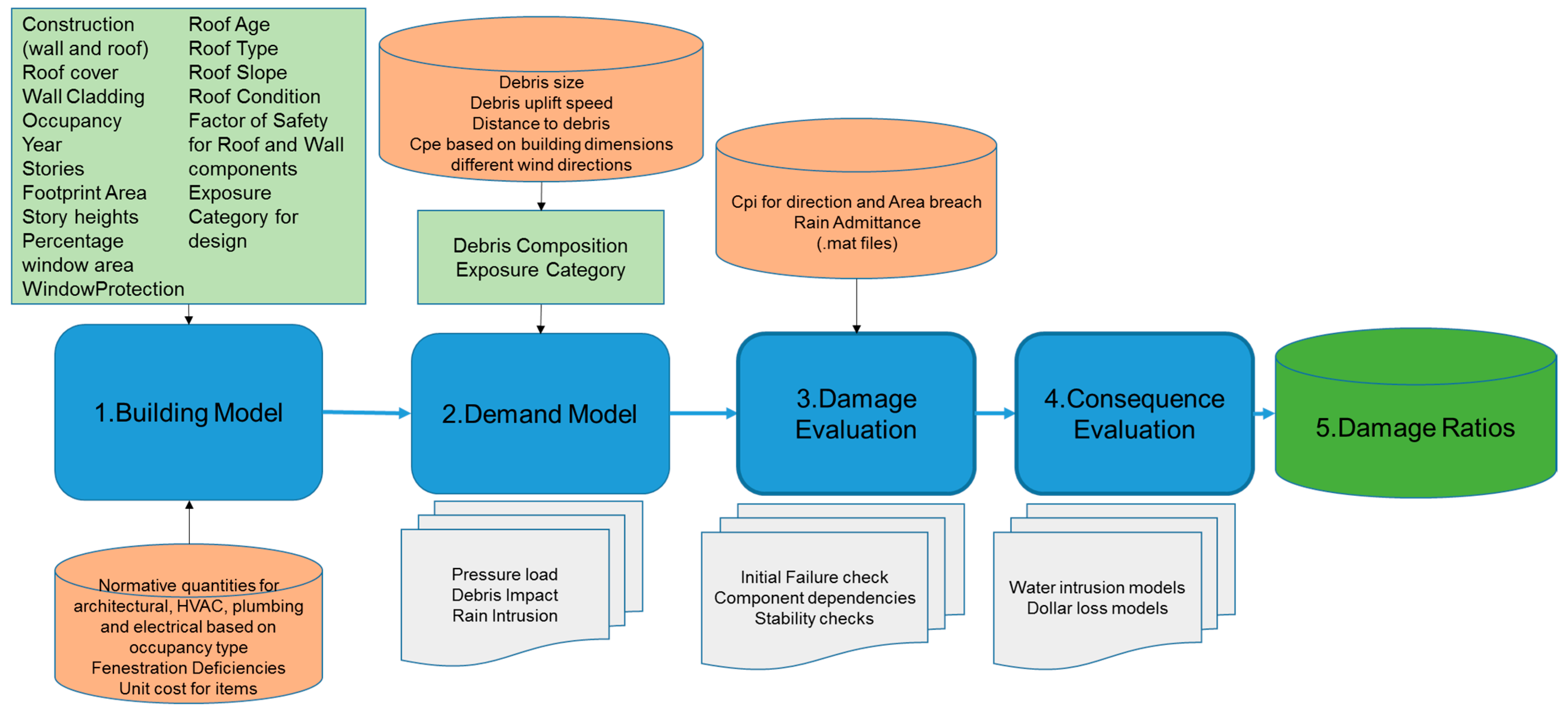
2. Materials and Methods

The damage ratio of a building can be represented as a function of wind speed, material properties, debris environment and properties of rainfall as shown below.

$$DR=f(M,W,R,C)$$

(1)

Here, M represents the material properties which includes wind uplift performance, debris impact resistance and resistance to rain intrusion. W represents the wind load acting on the components, which is a function of the wind speed, terrain and geometry of the building. R represents the properties of the rain, which is critical for determining the amount of rainwater intrusion and interior loss; C represents the cost of installation of individual components of the building used to determine the value of the building and repair cost. The framework and variables for the catastrophe model should be able to accommodate the variety of categories and sub-categories of elements of the building. The proposed framework runs as a five-step process as shown below in Figure 1. The five important steps [11,12,13,14,15,16,17] are: 1. Building Model 2. Demand Model 3. Damage Evaluation 4. Consequence Evaluation and 5. Damage Ratio evaluation. The main variables used in the models are listed in

Table 1. Description of variables.

Variable	Description	Units
DR	Damage Ratio	-
P0	Estimated mean capacity of the component	psf
$\phi$	Factor of Safety of a component	-
P	Nominal load on the component determined based on ASCE 7	psf or lb
RFage	Reduction factor for age of the component	-
Cn	Normalized Condition for age	-
$\sigma$	Standard deviation of capacity	psf
$q$	Wind pressure	psf
kz	Topographic factor from ASCE 7	-
$w$	Wind speed	mph
GCpe	External pressure coefficient	-
GCpi	Internal pressure coefficient	-
z	Height to the location where wind speed is calculated	ft
zg	Nominal Height to the atmospheric boundary layer	ft
α	Power law exponent based on ASCE 7	-
$K$	Tachikawa number	-
$\rho$	Air density	lb/ft3
$g$	Acceleration due to gravity	ft/s2
hm	Thickness of the debris	ft
ρm	Density of the debris	lb/ft3
$x^{*}$	Dimensionless horizontal displacement	-
$x$	Debris flight distance	-
wd	Speed of debris	ft/s
$C$	Coefficient based on shape of debris	-
RAF	Rain Admittance Factor	-
Vi	Volume of rain water	ft3
$IR$	Intensity of rain	-
Afw	Area of failed window	ft2
di	Deficiency in window	-
Fij	Factor for rain water calculation	-
$\theta$	Angle of attack of wind	deg.
Arc	Actual failed area of roof cover	ft2
Ars	Actual failed area of roof sheathing	ft2
Apfrc	Area of failed roof cover projected in the vertical plane	ft2
Apfrs	Area of failed roof sheathing projected in the vertical plane	ft2
Rrc	Factor to address secondary rainwater penetration for roof	-
Di	Quantity of Damage to the ith component	ft2 or number
Qi	Quantity of the ith component in the building	ft2 or number
Ci	Cost of repair of the ith component in the building	Dollar
Nc	Total number of components in the building	-

.

This model primarily serves the purpose of insurance loss modeling, and the building description in the insurance portfolio may be detailed or abstract. Hence, the framework should be able to model buildings with limited descriptions and those with detailed descriptions. Monte Carlo (MC) simulation forms the core of the framework. The final results will carry the latent uncertainties in each of the variables described. The final products are obtained as functions of wind speed; these are equivalent to the peak gust for a given hurricane wind event at a location. An overview of the MC simulation to determine the losses is given in Figure 2.

2.1. Building Model

This section describes the main components of the building and their properties that are included in the model.

2.1.1. Variables in the Building Model

The main items of the building model are the dimensions of the building, the roof, window and wall components, discretization of the components and their resistance capacities. These values are basically derived from the key variables used as input to the building model. These key variables are: 1. Occupancy 2. Year of construction 3. Number of stories and 4. Construction type. These properties are also known as primary modifiers in the insurance industry’s terminology. These properties are chosen because they play important roles in determining the resistance of the building components, the dollar value of the building and repair cost after damage.

Other important variables are design wind speed, roof construction type, window protection, wall cladding, percentage area of windows, age of the roof, roof maintenance and debris environment. Multiple factors influence the loss; however, the scope of the study is currently limited to the above-mentioned variables. The quantity and capacity of the components are determined based on the variables. The roof components—roof cover and roof deck (or roof sheathing in case of residential wood construction)—are discretized as rectangular elements.

Mean Resistance Capacity for Wind Uplift

To develop a general capacity model, the best estimate of capacity recommended by the structural designer for construction is estimated. For a given year of construction, the design load on a particular component is determined using the ASCE 7 specification that was relevant to that year (say for a year of construction of 2011, we use ASCE 7-2010). Furthermore, it would be a reasonable assumption to assign a mean capacity to the component based on the capacity of the component prescribed by its manufacturer (P₀). This mean capcity can be related to nominal load using the following approach. Let us say P is the prescribed nominal load obtained from the relevant ASCE 7 using the design wind speed at the location of the building Then, factor φ, which will be referred to as Factor of Safety (in general, $\phi$ is the ratio of load factor to resistance factor), can be used to determine P₀. The estimated mean capacity is

$$P_0=\phi P$$

(2)

For each component (roof cover, roof sheathing (roof deck) etc.) we can determine the nominal load P from the relevant ASCE 7, and $\phi$ based on engineering judgement. Components that cover a large area will be discretized into elements. While the roof and wall components are assumed to be discretized, a window or door are assumed to be one unit each and each window or door will have its own capacity value. A glazed window or door should be assigned a pressure capacity. The discretized elements of any component will be assigned a capacity randomly sampled from a distribution with $P_0$ as the mean capacity. This approach is rational in general; however, we should also note that residential constructions may not adhere to all the requirements in specifications and observed capacities tend to deviate from those observed in commercial occupancy constructions, suggesting lower values of $\phi$ for residential compared to commercial buildings.

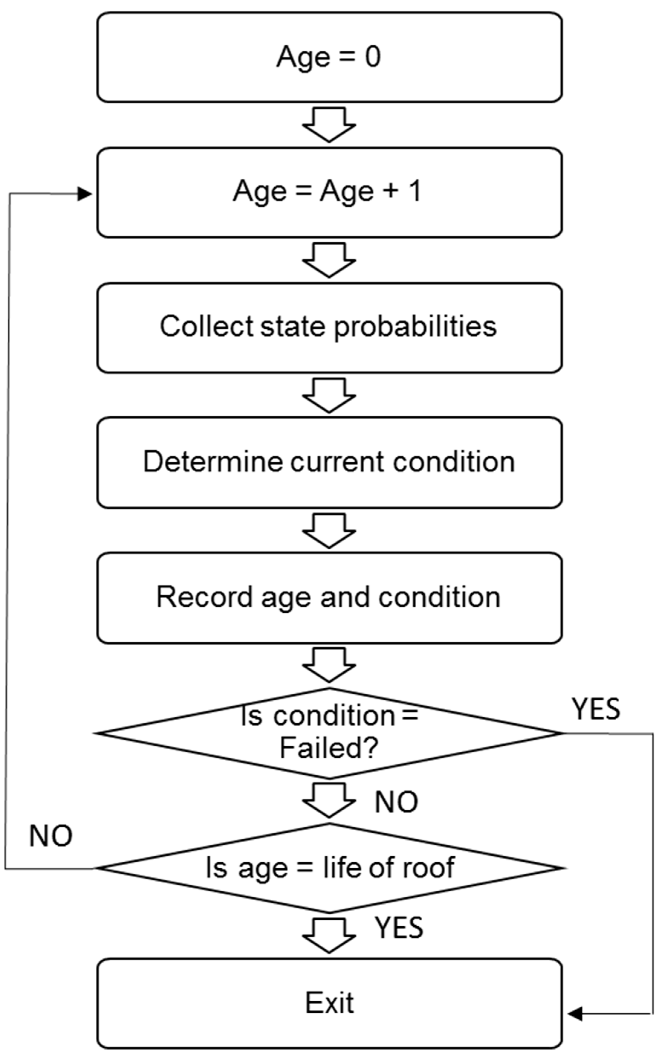
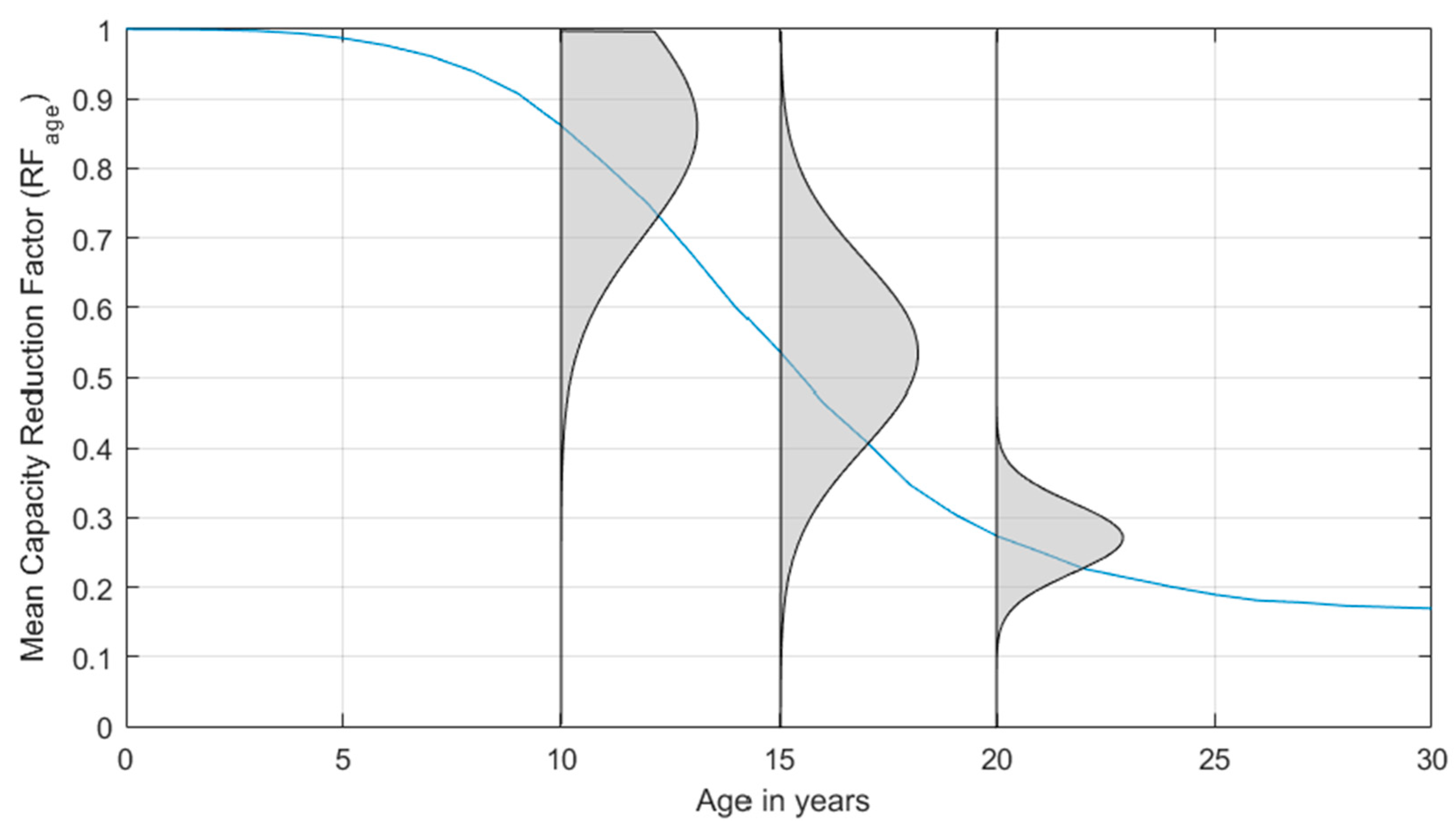
Roof Aging and Condition

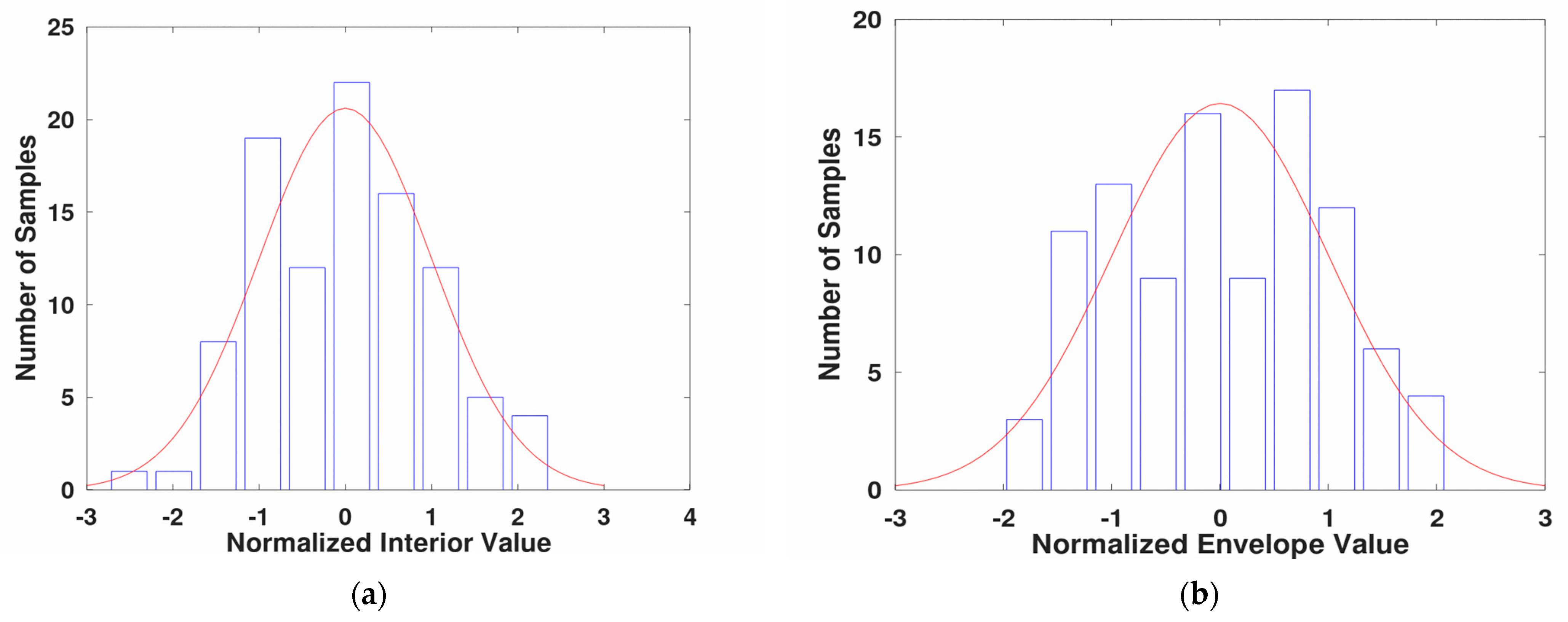
Roof aging and maintenance influences the performance of the commercial roof in protecting from water entry through the roof during hurricane events. Markov chain-based aging prediction models are popular in civil engineering [72,73,74,75]. Research focusing on aging of commercial roofs is available in [63,64,65]. Based on these studies, a Markovian roof condition change model is proposed to determine the average condition of the commercial roof with respect to age. We determine the reduction factor for the roof using a proposed logistic model (as shown in Equation (2), obtained using framework described in Figure 3 with respect to age.

Research on roof aging [63,64,65] reports roof conditions as ordinal data from extensive condition assessment surveys of commercial roofs. Based on the data, researchers also report state transition probabilities of the condition (on a scale of 1 to 7, where 7 is excellent) of in-use commercial roofs. These probabilities specify the likelihood that the roof will remain or change its state in unit time. We use these probabilities to model the performance degradation with time. A Markovian approach is adopted by determining the state transition probability based on data collected on roofs of in-use buildings [64]. Firstly, a Monte Carlo (MC) simulation was carried out using the state transition probabilities for a roof with a service life of 50 years. Simulation results for the 50-year-old roof match well with the values provided in [64] as shown in Figure 4a (compare Coffelt et al., 2008, and the 50-year simulation result). In order to determine the state transition probabilities for other roof lifespans, such as 20, 30 and 40 years, a linear model was implemented to update the probabilities. Repeating the MC simulation for all the service lifespan cases (20, 30 and 40 years), we obtain the results shown in Figure 4a.

Since we need to model the wind-resistance capacity of the roof and there are limited age-based uplift resistance data available, we have to model the capacity from the condition of the roof. Hence, the results from Figure 4a will have to be modified using a suitable model. A factor for capacity reduction is required to adjust the capacity of the roof for different state conditions (which are usually ordinal data in roof condition assessment surveys). Logistic models have been extensively used by researchers to model aging in materials (concrete, polymers and metals) in civil engineering [74,75]. Therefore, based on a literature review and engineering judgement, a logistic model was adopted to model a continuous capacity reduction factor starting from one at age zero for roofs of different lifespans as shown below in Equation (3). Here, C_n is the normalized condition factor of the roof. For example, for a roof with a lifespan of 50 years, after 10 years of use (please refer Figure 4a), C_n will be 3.3/7 = 0.47.

$$R{F}_{age}=1-4.35/(1+\exp (10C_n))$$

(3)

Based on the literature review [66,67,68,69,70,71], the relative measures of target capacities are met by the model results. The capacity obtained by the proposed model will be in the interval of 50% and 70% of the pristine capacity when the age of the roof reaches half of its lifespan. The residual capacity at the end of its lifespan will be close to 20% of its original capacity. The proposed model meets this expectation for all cases except for the 20-year service life, where it is over-predicted by 18% after 10 years. Results are shown in Figure 4b.

Furthermore, the uncertainty across the mean is addressed by modeling the uncertainty as a function of condition. While detailed data are not directly available, several studies on the capacity of roof components are [66,67,68,69,70,71]. Henceforth, a judicious choice of 25% for the maximum value of Coefficient of Variation (COV) is employed for distribution of capacities at half the lifespan for each case based on this literature. An example distribution of capacity is shown below in Figure 5. The lifespan of the roof considered is 30 years.

$$P_{mean}=R{F}_{age}{P}_0$$

(4)

Here P_mean is the mean roof capacity for the particular building simulation, obtained after multiplying the RF_age (the reduction associated with the age of the roof) to P₀ (as described in Equations (2) and (3)). The resistance capacities for the discretized elements of the roof are sampled from a Gaussian distribution based on [13,40]. The capacity of an ith element on the roof can then be assigned a capacity as shown below.

$$p(P_i)=N(P_{mean},{\sigma }^2)$$

(5)

Interior Value

The normative quantities reported in FEMA P58 [76,77] are used to determine the interior value. Normative quantities give the quantity of non-structural items available for the unit area or unit volume of the building. FEMA P58 Methodology reports the 10th, 50th and 90th percentiles of these items. The main items include Architectural trades on walls and floors, HVAC, Stairs, Elevators, Electrical and Fire protection. For a particular building occupancy type, the value of the interior (VI) of the building is determined using FEMA P58-1 50th percentile normative quantities for that occupancy type and RSMeans Data for the unit price. VI influences the DR calculation, since it increases the value of the building and also the possible damage that rainwater can cause to the interior. Needless to say, if the value of interior differs considerably for two buildings with similar envelope constructions and capacities, their damage ratios will also be different. Hence, it is important to model the interior value based on occupancy and dimensions of the building.

We use the 50th percentile values of non-structural components reported in FEMA P58 normative quantities to estimate the quantity of non-structural components. The total quantity of each component in the building is found by multiplying the per-square-feet quantity by the total area in square feet of the building. The Appendix A shows selected normative quantities and corresponding RSMeans rate [78]. The unit cost for each item is selected from the RSMeans database. The total quantity of one component multiplied by its unit cost will give the dollar amount for that component. Upon adding the dollar amount for all non-structural components, we obtain the total value of the interior of the building. The distribution of interior value from one hundred samples is shown in Figure 6.

2.2. Demand Model

The building under study will be subjected to wind loads of increasing intensities, one wind speed at a time. Each wind speed will be applied from different directions of the building as schematically shown in Figure 7. Wind pressure, debris impact and rain intrusion possibilities will be evaluated for each wind speed.

2.2.1. Wind Pressure Load

The loads on the components will be determined assuming a quasi-static approach following ASCE 07-10. The formula for the wind load on the components and cladding is used here:

$$q=0.00256k_z{w}^2(GC{p}_e-GC{p}_{{}_i})$$

(6)

The value of $k_z$ is determined using the formula given in ASCE 7-10, Table 28.3.1.

$$k_z=2.01{(\frac{z}{z_g})}^{(\frac{2}{\alpha })}$$

(7)

Here, $z$ is the height of the component, $z_g$ is the nominal height of the atmospheric boundary layer and $\alpha$ is the power law exponent. Each region of the roof (as shown in Figure 7) or wall is assigned a mean pressure coefficient and the discretized elements of each region of the roof can each be assigned a pressure coefficient.

2.2.2. Debris Impact

Based on the knowledge from recent studies [40,41,42,43,44,45,46,47,48,49,50] an efficient computational model is developed. A Tachikawa number is used to model the speed of the debris at each wind speed. The speed of the debris before hitting the target is modeled based on [48,50]. The density, mass and dimension are based on the data in [44,47]. The maximum percentage of potential debris hitting the building is fixed at 60%, based on [40].

$$K=0.5\rho w^2/(g{h}_m{\rho }_m)$$

(8)

$$x^{*}=gx/w^2$$

(9)

$$w_d=w(1-\exp (-\sqrt{2CK{x}^{*}}))$$

(10)

Descriptions of variables are available in the nomenclature table. The number of potential elements of debris is initially assigned. Then, the percentage of debris hitting the building is determined as a function of the wind speed. The debris that hits the building and target location on the building are randomly sampled. If any debris hits the window, the property of that debris is recorded. The ratio of momentum of the debris and the capacity of the protected window is calculated [71] for every element of debris that impacts the window. If the sum of the ratios for all the impacts is greater than one, then the window is marked as failed. The model is validated using the results from [10] as shown in Figure 8. Furthermore, the failure probability for protected and unprotected windows in two different environments is presented—a small-missile environment and a large-missile environment.

The results from the proposed model replicate the trend observed in Cope, 2004 for small-missile and large-missile environments. Since the unprotected window has a very low resistance to debris impact, it is expected that the failure probability will be similar for both cases. However, failure probability decreases from 0.5 (unprotected) to about 0.1 (protected) at 150 mph in a large-missile environment. If there is a breach in the envelope (window, door or wall) due to debris impact or pressure failure, the internal pressure is modified [24,25,26,33,37]. Properties of the breach, which include the area and location of the breach with respect to wind direction (for example windward or leeward wall), are required to modify the internal pressure.

After the internal pressure is modified, another envelope breach check is carried out using the new internal pressure. If there is any additional failure, the internal pressure is modified again. This continues until stability is reached. A final record is taken for component damage to obtain component-wise damage for the given building for a given wind speed and direction.

2.2.3. Rain Intrusion

Hurricane events possess a risk of wind-driven rain, which causes water intrusion into the building. Losses due to rain intrusion depend on the following main factors [56,57,58,59,60,61,62]: the intensity of impinging rain, spatial distribution of rain around the building and deficiency in windows and doors.

Impinging Rain

The quantity of impinging rain is conservatively modeled based on [56] as a function of wind speed. The average quantity of rain in inches is modeled as shown below.

$$IR=12.013\log (w)-44.4$$

(11)

Here, w is the wind speed in meters per second.

Distribution of Rain across the Surface of a Building

Rain admittance factors (RAF) values from [57] are used across the surface to incorporate the differences in rain intensity at different locations on the surface of building.

Area of Envelope Failure

The damaged roof-cover area contributes to water intrusion into the roof sheathing. Failure of roof sheathing leads to water intrusion into the building [11,12,13,14,15,16,17]. For wall components, it is conservatively assumed that, upon the failure of a window due to debris impact or pressure, the entire window or door area will contribute to wind-driven rain.

Deficiency in Windows and Doors

The deficiency along the edges of windows and doors acts as an entry point for wind-driven rain [56]. The deficiencies in windows and doors are obtained as factors using the ASHRAE data [56]. We use the deficiencies d_i for each window.

$$V_i=IR RAF A_w d_i$$

(12)

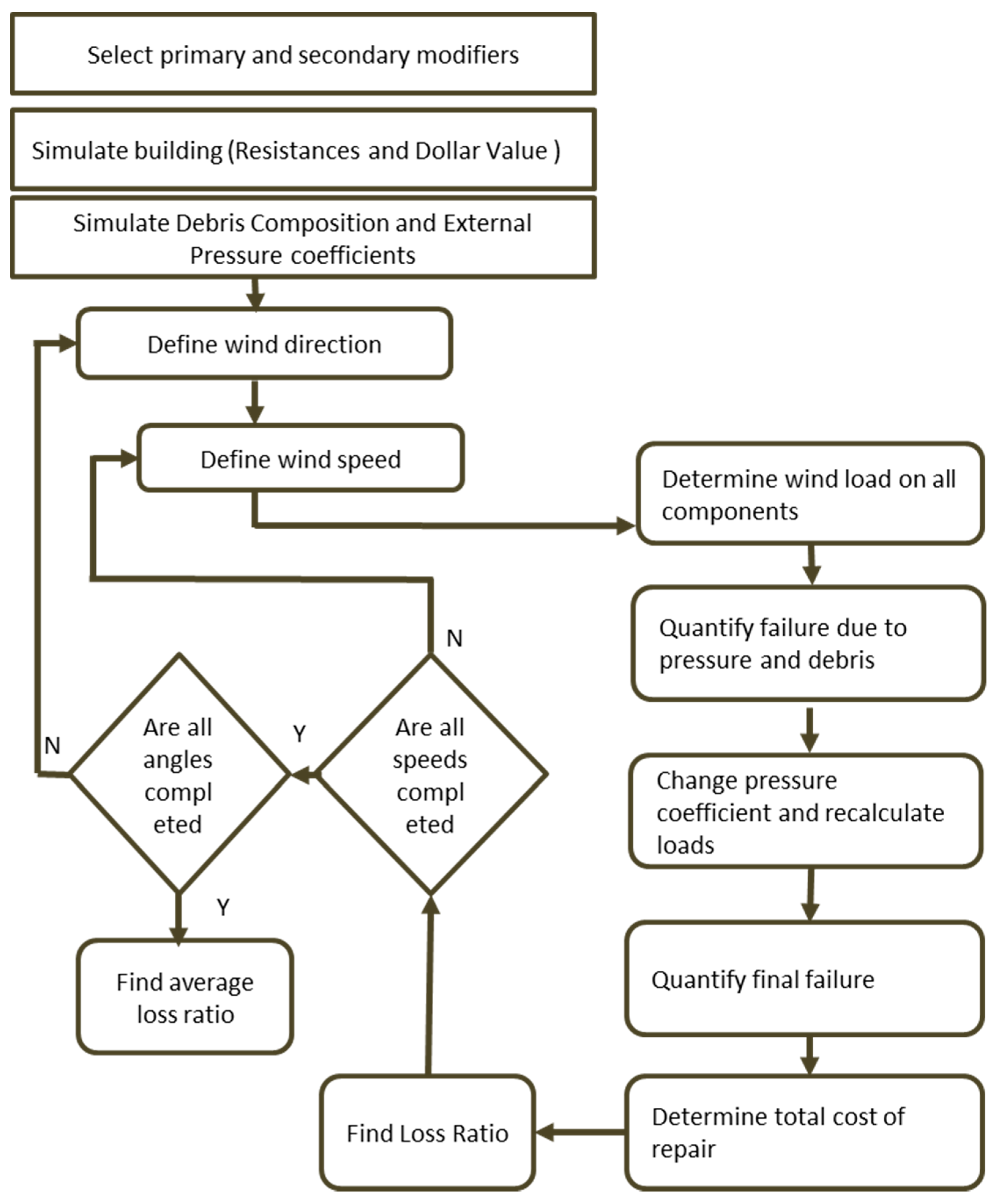
2.3. Damage Evaluation

The following steps are carried out to determine the failure

• Initial failure check: each component of the building is checked for failure for a given wind speed and wind direction. Any component that is failed is recorded. Dependency of the roof cover on the roof deck is considered in this check along with the dependency of the roof sheathing on roof-to-wall connections.
• Recalculation of internal pressure if the envelope is breached: if the envelope is breached, the internal pressure coefficient is recalculated based on the area of failure and wind direction [24,25,26,33,37].
• Recalculate the loads on the components and check for equilibrium: the loads on the components are recalculated, using the new internal pressure. Using the new loads, each component is checked for failure. Since the internal pressure depends on the area and location of failure of the envelope, we need to recalculate load, internal pressure and area of failure until there is an equilibrium, which means there is no more failure of any components. At this point, the maximum damage that can happen to the building due to wind pressure and debris will be obtained. This amount of damage for all the components that are modeled is recorded for the particular wind speed. These values will be further used in the next steps to estimate dollar losses.

2.4. Consequence Evaluation

This includes the calculation of the amount of water that enters the building and the dollar loss that it can cause.

2.4.1. Quantity of Water Entering the Building

The amount of water accumulating in each floor is determined from the top to the bottom floor. The amount of water entering the top floor is determined as a function of roof cover failure, roof deck failure and fenestration failure in the top floor. The amount of water entering due to roof cover failure is obtained using the following method. The area of failure is obtained from previous steps.

A model is proposed for rain entering the building based on [50,51,52,53]. The amount of water that can enter the building after the roof cover failure and roof deck failure is found, accounting for surface runoff and rain entering the building directly [53]. The area of breach $A_{rc}$ or $A_{rs}$ is modeled as a square with one side along the edge of the roof. A hypothetical channel of water from the missing deck area to the ridge is considered. The length of the channel is from the top of ridge to the top corner of the square area. The depth of the water in the channel is determined in inches of rainfall, obtained from Equation (10). A factor of 0.03 is used, based on engineering judgement, to adjust the surface runoff and actual amount of water passing through the opening. Similarly, the volume of direct rain entering the building is 10% of the directly impinging rain. Combining the surface runoff and direct rain, the volume is found using Equation (12).

$$V_{ij}=F_{ij}IR\cos (\theta )(0.03B\sqrt{A_i}+0.1A_i)$$

(13)

$$i=1\mathrm{for}\mathrm{RC},i=2\mathrm{for}\mathrm{RS},j=1\mathrm{for}{A}_{rc}>=A_{rs},j=2\mathrm{for}{A}_{rc}<A_{rs}$$

$$F_{11}=1,F_{12}=0,F_{21}=F_{22}=10$$

Apparently, during the wind event, the rain is horizontal. Hence, the quantity of rain entering the inside of the building is determined using the projected vertical area of roof cover and roof deck failure. The quantity of water entering each floor is determined by summing up the individual contributions and water that percolates from the floor immediately above it. The water percolating to the next level will be subtracted. Equations (14) and (15) give, respectively, the volume of water entering the top story due to roof cover and roof deck failure.

$$V_{RCi}=IR A_{pfrc} R_{rc}$$

(14)

$$V_{RSi}=IR A_{pfrs}$$

(15)

Percolation to the floor below is modeled as per [56] as 12% of the water accumulating in the given floor.

$$V_{}=IR A_{pfrs}$$

(16)

Typical floor—water entering from damaged windows for this floor and water percolating from the top floor will be calculated. The amount of water percolating to the floor below will be subtracted.

First floor—the water entering through breached doors, windows of this floor and water percolating from the floor above will be added up.

2.4.2. Dollar Loss

When the volume of water entering a floor can cover one inch of depth for the entire floor, the whole value of the floor is marked as a total loss [13,56]. Losses due to water intrusion to the interior are modeled as a polynomial function for a depth less than 1”.

2.5. Damage Ratio Calculation

The damage ratio is defined as the ratio of repair cost of the damaged components to the total replacement value of the building. The envelope repair cost is found by multiplying the unit cost of repair by the loss and adding up the repair costs for each component. The interior repair cost is found as a function of the depth of water that enters the building.

$$DR={\displaystyle \sum _i^{Nc}(D_i{C}_i)/}{\displaystyle \sum _i^{Nc}(Q_i{C}_i)}$$

(17)

$DR$ is the total damage ratio for the building.

$D_i$ is the amount of damage to the ith component.

$C_i$ is the unit cost of replacement for the ith component.

$Q_i$ is the total quantity of the component.

$N_c$ is the total number of components.

Dollar loss to interior: to determine the dollar loss due to water intrusion, the depth of water in each floor is determined by dividing the total volume of water in each floor with the floor area. Dollar loss is modeled as a polynomial, reaching one hundred percent of the floor when the depth of water for the entire floor is one inch. Finally, the cost of repair, for the envelope and interior, is divided by the total value of the building to obtain the damage ratio. This calculation is carried out for eight directions (45-degree increments) and one hundred simulations, which results in 800 damage ratio values for each wind speed. The average of eight directions is found for each wind speed. In the next section we demonstrate an example, present validations and use model results to demonstrate the influence of attributes.

3. Results

In this section, we first ensure that the simulations converge. Then, the results from the proposed model are validated using the examples from public models and insurance claims data from Hurricane Andrew. Furthermore, the influences of different attributes are investigated using the proposed model for a commercial occupancy example.

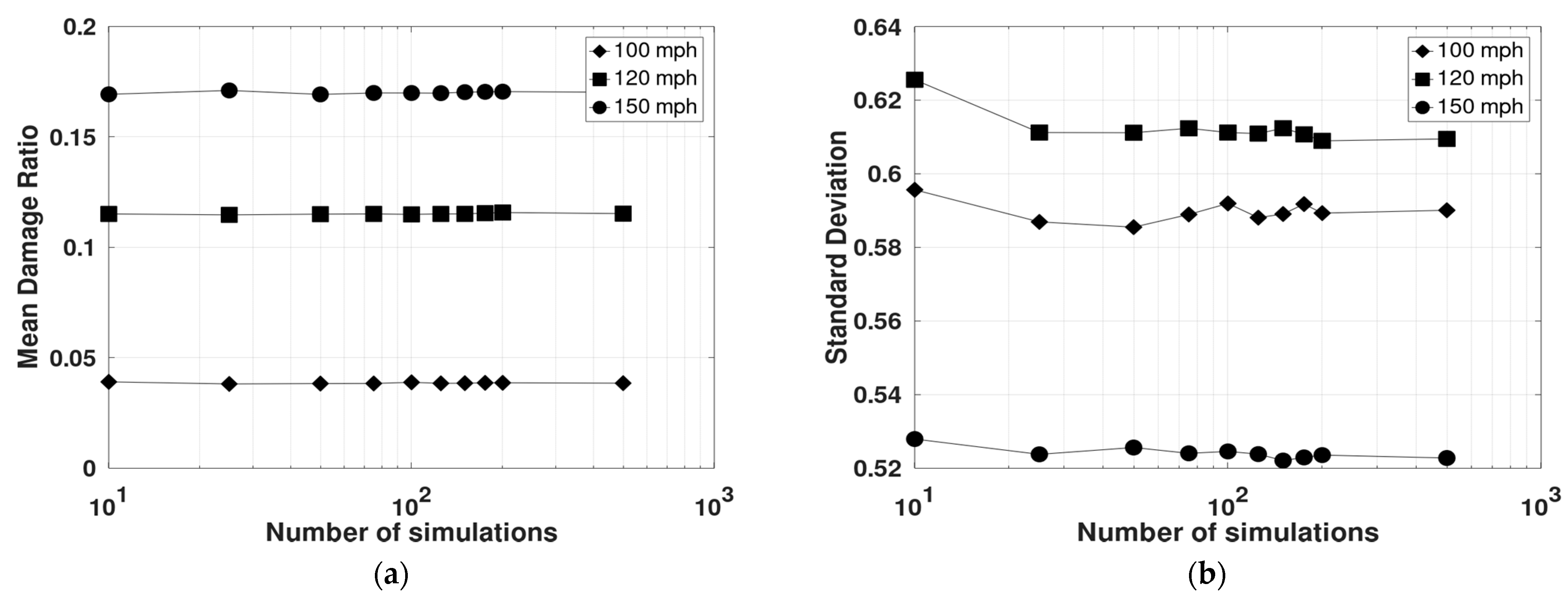
3.1. Convergence of Simulations

In order to ensure that the simulations can reproduce results consistently, the stability of the results is verified for a different number of simulations for a commercial office building. Results are given in Figure 9.

The mean DR was found to converge with 100 simulations and the percentage change is less than 1% when simulations were increased from 100 to 1000. The percentage improvement in the standard deviation is close to 2% when simulations were increased from 100 to 1000. Hence, 100 simulations is identified as a suitable number of simulations for the framework. If the simulations do not converge after 100 runs, it is recommended to run 1000 or more simulations until the results converge.

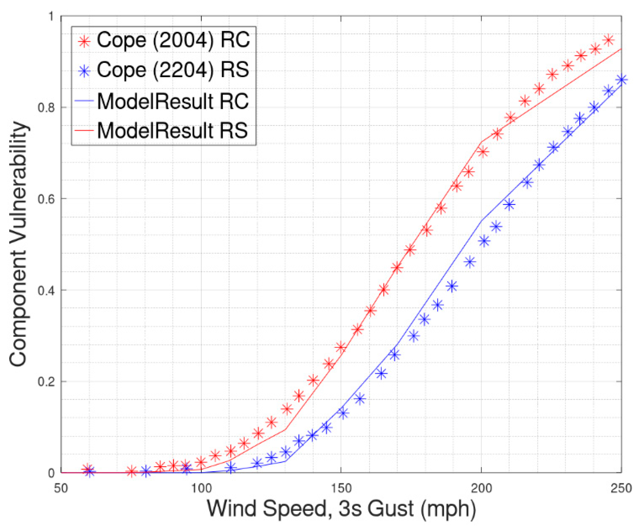
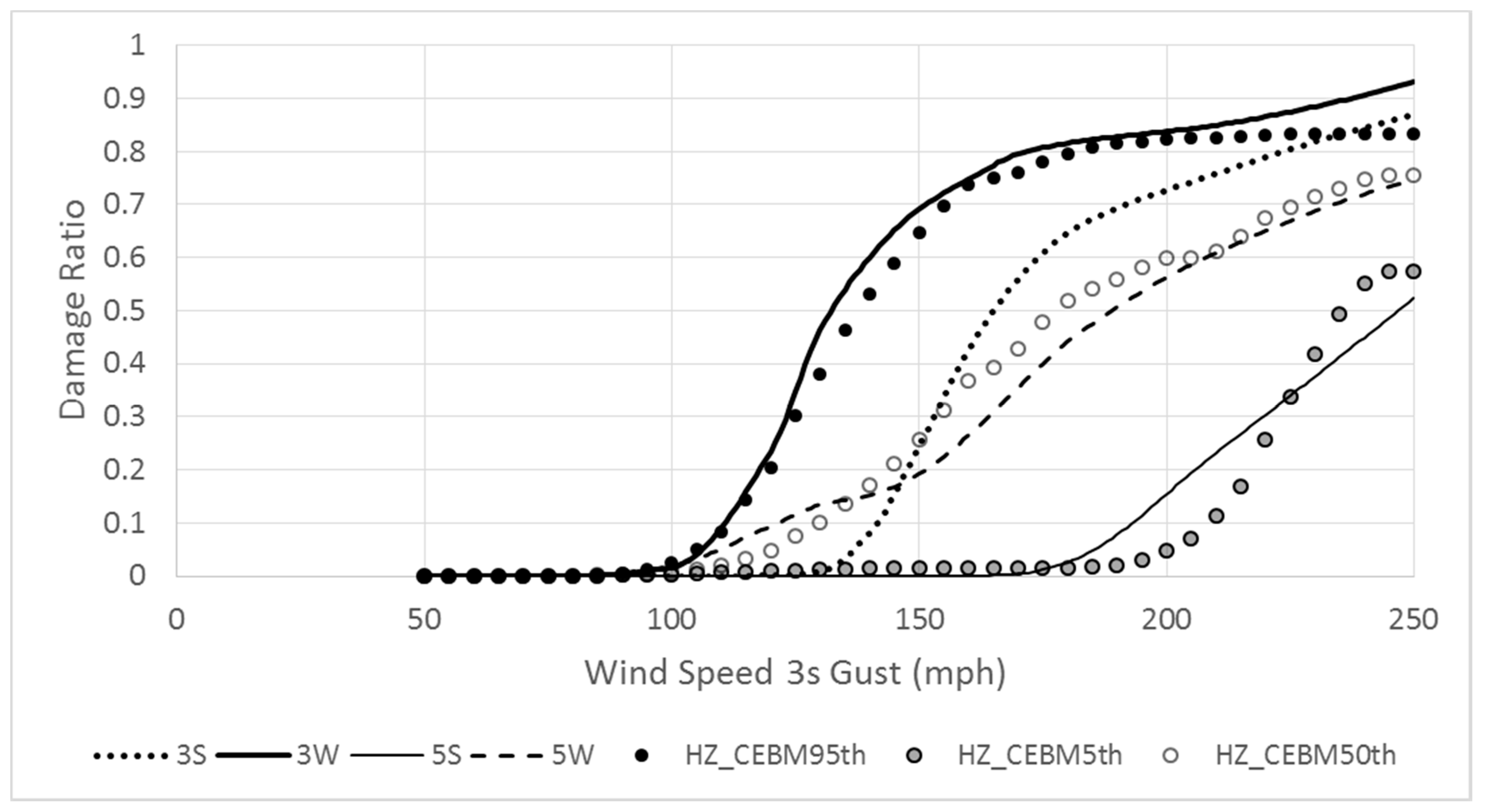
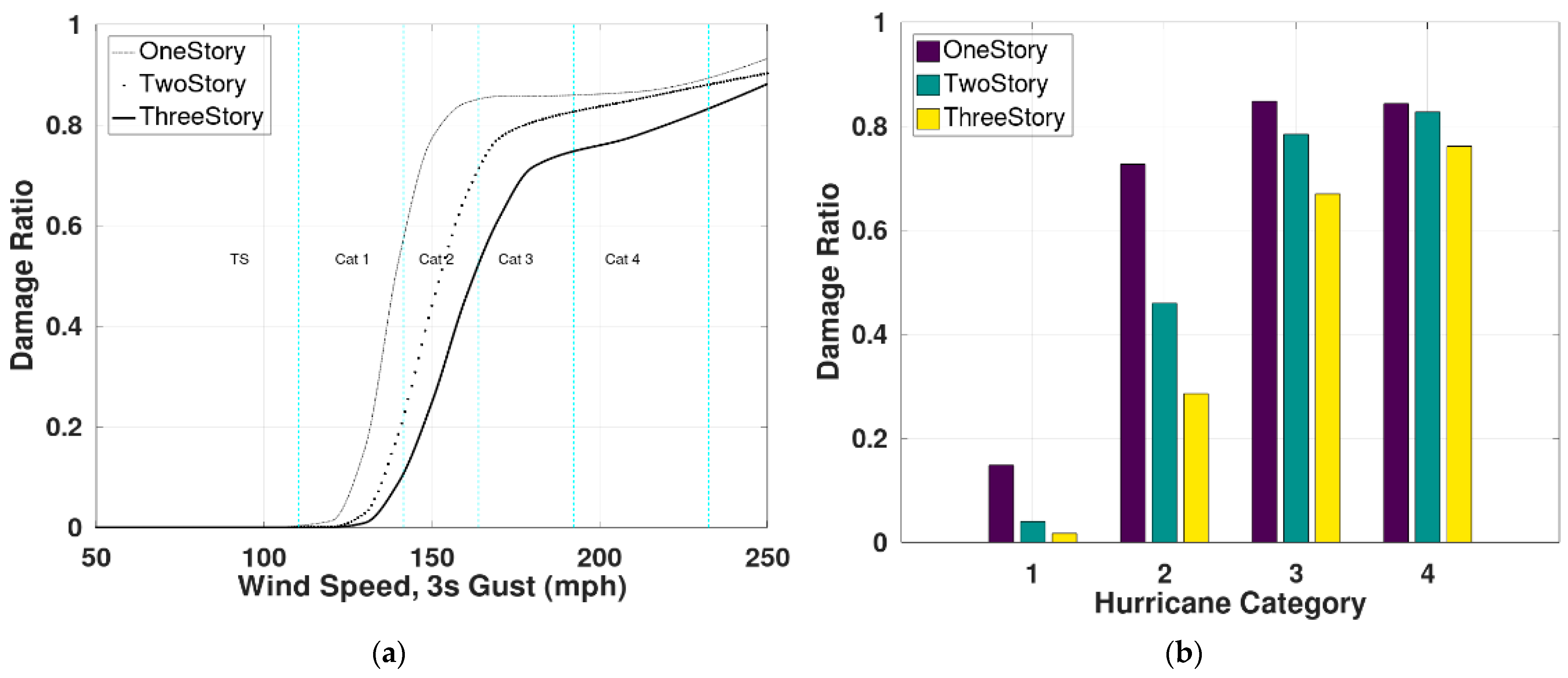
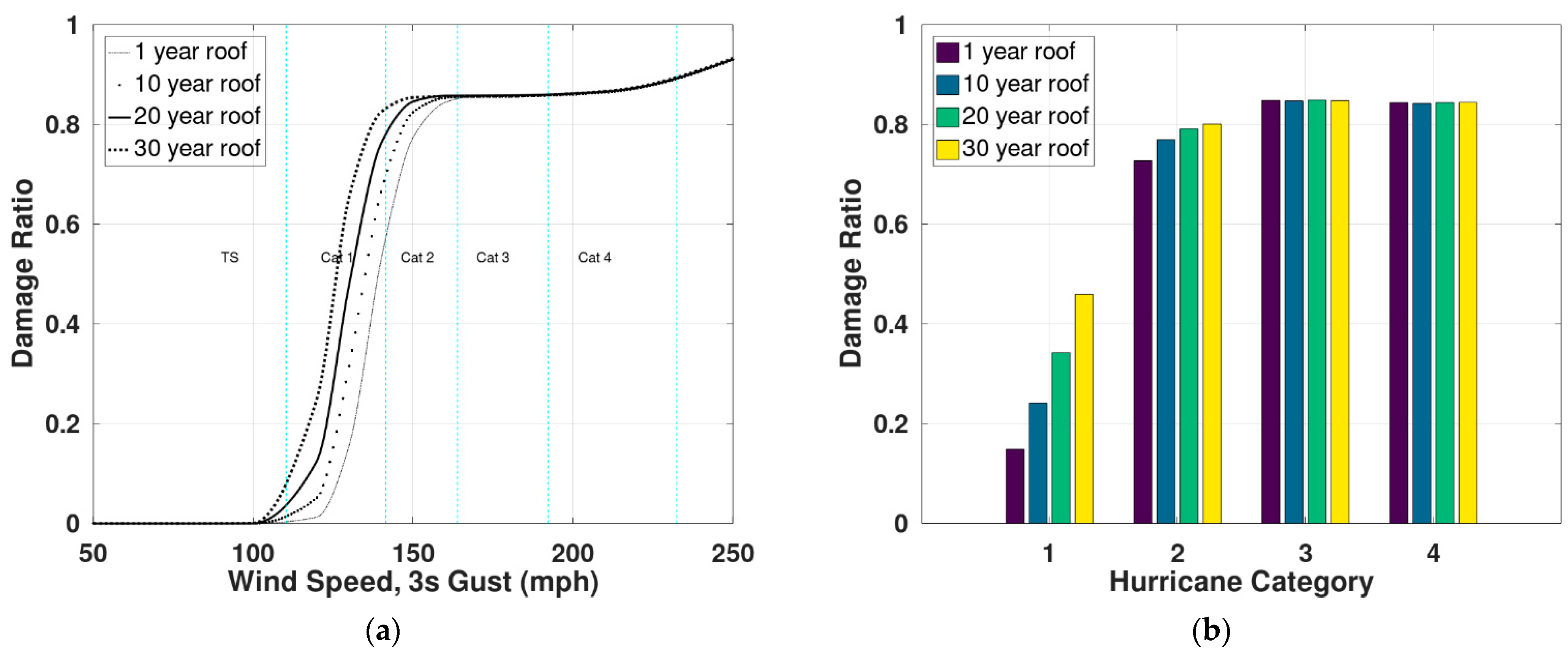
3.2. Case Study 1: Residential Building

In order to validate the accuracy of the model, an example study from [13] is carried out. The building has a length of 56 ft and breadth of 44 ft. This is a wood, gable roof-type building with a roof slope of 5:12 and design speed of 100 mph. More details about the input values are given in

Table A1. Attributes of the buildings used as inputs for example 2 are listed below.

Attribute Name	Residential (Case Study 1)	Strong (Case Study 2)	Weak (Case Study 2)
Occupancy	Single Family	Office	Office
Construction	Wood	Concrete	Concrete
Year	1997	1997	1997
Number of Stories	1	3,5	3,5
Floor Area	2464	10,000	10,000
Aspect Ratio	1.64	3	3
Roof Geometry	Gable	Flat, with basic slope	Flat, with basic slope
Roof Slope	5/12	1/12	1/12
Roof Maintenance	Excellent	Excellent	Excellent
Hurricane Bracing	Adequate	Adequate	Adequate
Opening Protection	No	Large Debris	No
Height Ground	10	12	12
Height Typical	0	10	10
Height Top	0	10	10
Exposure Category for Design	C	C	C
Exposure Category for Load	C	C	C
Design Speed	100	100	100
Debris Percentage Small	90	90	90
Debris Percentage Medium	5	5	5
Debris Percentage Large	5	5	5
Wall Cladding Type	Vinyl Siding	Brick Veneer	Brick Veneer
Percentage Window Area First Floor	10	20	20
Percentage Window Area Typical Floor	0	20	20
Percentage Window Area Top Floor	0	20	20
Roof Factor of Safety in Main region	1.5	1.5	1.0
Roof Factor of Safety in Corner region	1.2	1.5	1.0
Roof Factor of Safety in Edge region	1.2	1.5	1.0
Roof Cover Capacity Distribution	Lognormal	Gaussian	Gaussian
Roof Insulation Capacity Distribution	NA	Gaussian	Gaussian
Roof Deck Capacity Distribution	Lognormal	Gaussian	Gaussian
Roof cover COV	0.4	0.1	0.1
Roof Sheathing COV	0.4	0.1	0.1
Wall FS Main	1.2	2	1.5
Wall FS Corner	1.2	2	1.5
Wall Capacity Distribution	Gaussian	Gaussian	Gaussian
Wall COV	0.4	0.1	0.1
Window Capacity Distribution	Gaussian	Gaussian	Gaussian
Window COV	0.2	0.1	0.1
Window FS	1.16	2	1.5

for this case study. Figure 10 shows the three-dimensional plot of the study building and the contour of pressure coefficients on the surface of the building, generated for one sample simulation.

The pressure coefficients are simulated from the mean value and the coefficeint of variation (COV) using the probability distribution obtained from [13]. For each wind speed and direction, the pressure coefficients are randomly sampled using a Gaussian model. Component vulnerability shows the extent of damage that can happen to a particular component for a given wind speed and is averaged across all wind directions. After completing the simulation, the component vulnerability of the roof cover and sheathing was compared for this study. The results (Figure 11) show a good match between the vulnerability of the components (roof cover and roof sheathing) from [13] and the proposed model.

3.3. Case Study 2: Commercial Buildings Based on HAZUS Models

This Case Study compares HAZUS vulnerability functions for commercial concrete (low- and medium-rise buildings) in open terrain with the model results. The purpose of this study is to verify whether the model can replicate the qualitative trend observed in HAZUS loss functions. The proposed vulnerability framework is used to model 3- and 5-story offices with concrete walls and roofs at a design speed of 100 mph. The input variables were based on a HAZUS technical report [12]; however, exact values of all the variables are not available and engineering judgement was used to fill the missing input variables. A detailed list of the input data is shown in Table A1 and

Table A2. Inputs for Debris impact model.

Attribute Description	Numerical Values	Units
Distance to source of debris	[10,35]	feet
Debris uplift wind speed limits	Small [80,110] Medium [130,160] Large [140,170]	mph
Debris C value	0.8, 0.496, 0.9
Momentum capacity of unprotected window	0.025	kgm/s
Momentum capacity of protected window	62.37	kgm/s

in Appendix A. Four combinations were obtained: 3-story weak, 3-story strong, 5-story weak and 5-story strong. Results simulated using the proposed model for each case are compared with the 5, 50 and 95th percentiles of HAZUS vulnerability functions. The results (Figure 12) show that the proposed model captures the general trend observed in the HAZUS loss functions database.

Strong buildings are modeled to exceed the design criteria factor of safety and are modeled with windows that can sustain large debris impacts. Weak buildings do not meet the factor of safety for design criteria and windows are vulnerable to small debris attacks. Properties of the proposed models are shown in Table A1 in Appendix A. The results show that the model is well-capable of replicating the qualitative trend observed in the HAZUS loss functions database for mid-rise buildings. However, the results will not match closely because the proposed analysis methodology is different from HAZUS.

3.4. Case Study 3: Influence of Primary and Secondary Modifiers

Primary modifiers are considered to be significant drivers of loss in insurance industry circles. The influence of primary modifiers on DR is shown below. This include Construction, Occupancy and Number of stories. While the year of construction is a primary influencer, it is not included in the study here. Given below are the vulnerability functions from multiple cases and the average losses for each hurricane category obtained by averaging the vulnerability function in the interval of the Saffir-Simpson wind speeds for each hurricane category. This averaging helps to compare the DRs for multiple buildings easily.

a. Number of Stories: model results from Figure 13 show that, in general, DR decreases with an increase in the number of stories for a given wind speed. A single-story building is more vulnerable than a two-story building. While roof and window damage will not deviate significantly from each other for single- and two-story buildings, single-story buildings are more susceptible to interior damage, primarily because of the concentration of interior value in a single floor. Hence, water intrusion and subsequent dollar loss increases rapidly in the single-story building compared to the two-story building. On an average the DR from the model was found to be 0.14, 0.04 and 0.02 for one-, two- and three-story buildings respectively for Cat1 hurricanes, while it is 0.71, 0.46 and 0.25 respectively for Cat2 hurricanes.

b. Construction type: the model results from two different wall construction types are shown below in Figure 14. Reinforced concrete buildings are less vulnerable compared to masonry buildings. The average DR and percentage change with respect to reinforced concrete buildings are shown below in the table.

The influences of secondary modifiers were tested using the proposed model to ensure the model meets the expected outcomes for each modifier type. This study will enable the exploration of the future research possibilities of the model and to understand the approach for the model calibration.

c. Opening Protection: the debris impact protection was compared for large debris impact-rated windows and windows with no debris impact protection, as shown in Figure 15. All stories are modelled with windows rated for large debris impact protection. Also, in this study, the debris impact model considers the probability of missiles striking in each story. This example compares two similar buildings, one with debris impact protection and other with no debris impact protection. The model results show that the influence of window protection is significant in the 100 mph wind speed to design speed (3 s peak gust) regime. Here a factor of safety of 1.5 (

Table A3. Selected Normative quantities of selected items and their unit rates from RSMeans shown as an example. More details can be found in FEMA (2012) and RSMeans 2013.

Item	Unit of Measurement	Normative Quantity (50th Percentile)	Unit Rate as Per RSMeans 2013 ($)
Interior partition length	100 LF per 1 gsf	1 E-3	10/ft
Ceramic Tile floors	SF per 1 gsf	0.042	4.3/sf
Ceiling Lay in Tile	%	95	1.8/sf

) and a design wind speed of 130 mph are used to estimate the capacity of the roof cover and roof deck for both the buildings. The results indicate that a lack of window protection can be a significant driver of loss in the Cat1, Cat2 and Cat3 hurricane wind speeds for the vulnerable building. So, even if all the building components meet or exceed the design wind speed demand, but the windows do not meet the debris impact standards, then such buildings could experience losses of 5%, 15% and 30% at Cat1, Cat2 and Cat3 wind speeds respectively. Impact-resistant windows will reduce the losses by 66% for Cat3 and by 100% for Cat2 and Cat1 hurricane. In addition, losses in buildings with no window protection and a high-debris environment are also presented. The losses can go up by almost 100% at 150 mph in a high-debris environment.

d. Roof aging: as per the model, the aging of the roof can influence its performance, and hence, the DR induced in the building as shown in Figure 16. Roof retrofit to improve performance is not considered in this study. Aging of the roof increases losses, averaging at 0.05, 0.6 and 0.12 for 10-, 20- and 30-year-old commercial roof for Cat1 hurricanes. Similarly, the DR is 0.3, 0.45 and 0.5 for Cat2 hurricanes. The difference diminishes thereafter.

e. Floor Area: it was also observed (from Figure 17) that footprint area does not influence the model result significantly. There has been research indicating that buildings with larger floor areas tend to have lower damage ratios when compared to buildings with smaller damage ratios. This model shows DR at 0.1 and 0.15 at Cat 1 for 10k square feet and 20k square feet, respectively. However, this study finds that the influence of floor area on DR is not significant compared to other modifiers discussed earlier.

4. Discussion

A wind vulnerability framework was proposed, which was used to generate loss functions for residential and commercial buildings. The proposed framework enables loss modeling based on a component vulnerability approach and without considering the fragility of the building components as such. The new contributions include a Markovian roof aging model and normative quantities from FEMA P58 for each occupancy type. The resistance capacity of the building components is determined based on design wind speed and the relevant ASCE 7-10 code. The modelers can adjust the component capacities by engineering judgement of the factor of safety depending on the perceived quality of the construction. Roof aging and roof maintenance factors are modeled using a Markovian model, which enables the loss modeler to choose which inputs can be provided based on the knowledge they have about the building. This knowledge may come from the year of the last renovation of the roof, or an inspection of the roof. Similarly, the modelers can also choose the inputs for the debris impact resistance of windows and water intrusion criteria. Thus, the model provides more flexibility in modeling risk using the input parameters. The initial results are promising; however, further validation with insurance claims data and component failure data (such as roof cover or cladding), and calibration may be required to make the model more robust. The framework and software modules are well organized, and any changes or additions in the framework can be easily implemented in the software platform. At present, the framework considers the vulnerability of roof-to-wall connections but does not consider the failure of main structural elements such as beams, slabs and columns. Hence the model has a limitation that it will not be able to replicate the results observed for cases of structural failure under wind loads. The main highlights of this study are:

• A framework for generating vulnerability functions to assist insurance loss modeling has been proposed, which, unlike conventional models, does not rely on the fragility of components. Results were validated using the residential building examples from FPHLM and a commercial building example from HAZUS. The influence of primary modifiers (story and construction) and secondary modifiers (window protection, roof age, and debris composition) on overall loss was also explored.
• A Markovian approach-based roof aging model is introduced, which is able to predict the increase in vulnerability with aging. Further study based on claims data is necessary to validate the results of the model or to calibrate the model as necessary. The state transition probabilities used in the analysis can also be modified if new data are available from in-service roofs.
• Damage ratio was found to decrease with an increase in the number of stories by about 50% for Cat1 hurricanes for each added story. Floor area does not influence losses significantly.
• Reinforced concrete buildings are about twice as resilient as masonry for Cat1 hurricanes.
• The model also shows that window protection can help to mitigate losses induced by debris impact in different debris environments. It can reduce losses for Cat2 hurricanes by 100% and Cat3 by 66%.

The initial results from this study are very promising, and validation with actual losses paid is important in the future. It should be noted that post-hurricane claims data (which are the actual compensation paid to the customers) may not show a similar trend, mainly due to the fact that claims data are not well detailed (for example, number of stories, actual value, amount of damage to roof, windows or walls) and could often be polluted unintentionally because losses from other causes (such as a flood) could be counted as wind-induced losses. Future work will include validation of DRs using good-quality claims data and investigating the influence of the year of construction while considering the effect of aging on roofs and other components as well. Moreover, future work will also involve regional study integrating wind hazards and vulnerability modules to study the influence of engineering properties and envelope retrofit on financial loss during hurricane events in a study region. Integrated models can also be used to study long-term and short-term financial risks in any study region for insurance risk management.

References

1. Rosowsky, D.V. Projecting the Effects of a Warming Climate on the Hurricane Hazard and Insured Losses: Methodology and Case Study. Struct. Saf. 2021, 88, 102036. [Google Scholar] [CrossRef]
2. Pachauri, R.K.; Allen, M.R.; Barros, V.R.; Broome, J.; Cramer, W.; Christ, R.; Church, J.A.; Clarke, L.; Dahe, Q.; Dasgupta, P. Climate Change 2014: Synthesis Report. In Contribution of Working Groups I, II and III to the Fifth Assessment Report of the Intergovernmental Panel on Climate Change; IPCC: Geneva, Switzerland, 2014. [Google Scholar]
3. Van Vuuren, D.P.; Edmonds, J.; Kainuma, M.; Riahi, K.; Thomson, A.; Hibbard, K.; Hurtt, G.C.; Kram, T.; Krey, V.; Lamarque, J.-F. The Representative Concentration Pathways: An Overview. Clim. Chang. 2011, 109, 5–31. [Google Scholar] [CrossRef]
4. Why Hurricane Risk Modelling Has to Change|Swiss Re. Available online: https://www.swissre.com/risk-knowledge/mitigating-climate-risk/why-hurricane-risk-modelling-has-to-change.html (accessed on 11 January 2022).
5. Pinelli, J.-P.; Roueche, D.; Kijewski-Correa, T.; Plaz, F.; Prevatt, D.; Zisis, I.; Elawady, A.; Haan, F.; Pei, S.; Gurley, K. Overview of Damage Observed in Regional Construction during the Passage of Hurricane Irma over the State of Florida. In Forensic Engineering 2018: Forging Forensic Frontiers; American Society of Civil Engineers: Reston, VA, USA, 2018; pp. 1028–1038. [Google Scholar]
6. Zhou, Z.; Gong, J.; Hu, X. Community-Scale Multi-Level Post-Hurricane Damage Assessment of Residential Buildings Using Multi-Temporal Airborne LiDAR Data. Autom. Constr. 2019, 98, 30–45. [Google Scholar] [CrossRef]
7. Tilon, S.; Nex, F.; Kerle, N.; Vosselman, G. Post-Disaster Building Damage Detection from Earth Observation Imagery Using Unsupervised and Transferable Anomaly Detecting Generative Adversarial Networks. Remote Sens. 2020, 12, 4193. [Google Scholar] [CrossRef]
8. Herseth, A.; Ashley, E. FEMA Mitigation Assessment Team Program: Observations and Recommendations since Hurricane Andrew. In Advances in Hurricane Engineering: Learning from Our Past; American Society of Civil Engineers: Washington, DC, USA, 2013; pp. 630–645. [Google Scholar]
9. Mehta, K.C. Wind Induced Damage Observations and Their Implications for Design Practice. Eng. Struct. 1984, 6, 242–247. [Google Scholar] [CrossRef]
10. Keith, E.L.; Rose, J.D. Hurricane Andrew—Structural Performance of Buildings in South Florida. J. Perform. Constr. Facil. 1994, 8, 178–191. [Google Scholar] [CrossRef]
11. Clark, K.M. The Use of Computer Modeling in Estimating and Managing Future Catastrophe Losses. The Geneva Papers on Risk and Insurance. Issues Pract. 2002, 27, 181–195. [Google Scholar]
12. Vickery, P.J.; Skerlj, P.F.; Lin, J.; Twisdale Jr, L.A.; Young, M.A.; Lavelle, F.M. HAZUS-MH Hurricane Model Methodology. II: Damage and Loss Estimation. Nat. Hazards Rev. 2006, 7, 94–103. [Google Scholar] [CrossRef] [Green Version]
13. Cope, A.D. Predicting the Vulnerability of Typical Residential Buildings to Hurricane Damage; University of Florida: Gainesville, FL, USA, 2004. [Google Scholar]
14. Pinelli, J.-P.; Simiu, E.; Gurley, K.; Subramanian, C.; Zhang, L.; Cope, A.; Filliben, J.J.; Hamid, S. Hurricane Damage Prediction Model for Residential Structures. J. Struct. Eng. 2004, 130, 1685–1691. [Google Scholar] [CrossRef]
15. Hamid, S.; Kibria, B.G.; Gulati, S.; Powell, M.; Annane, B.; Cocke, S.; Pinelli, J.-P.; Gurley, K.; Chen, S.-C. Predicting Losses of Residential Structures in the State of Florida by the Public Hurricane Loss Evaluation Model. Stat. Methodol. 2010, 7, 552–573. [Google Scholar] [CrossRef]
16. Hamid, S.S.; Pinelli, J.-P.; Chen, S.-C.; Gurley, K. Catastrophe Model-Based Assessment of Hurricane Risk and Estimates of Potential Insured Losses for the State of Florida. Nat. Hazards Rev. 2011, 12, 171–176. [Google Scholar] [CrossRef]
17. Pan, F. Damage Prediction of Low-Rise Buildings under Hurricane Winds. Ph.D. Thesis, Louisiana State University and Agricultural and Mechanical College, Baton Rouge, LA, USA, 2014. [Google Scholar]
18. Mehta, K.C.; Smith, D.A.; McDonald, J.R. Procedure for Predicting Wind Damage to Buildings. J. Struct. Div. 1981, 107, 2089–2096. [Google Scholar] [CrossRef]
19. Sparks, P.R.; Schiff, S.D.; Reinhold, T.A. Wind Damage to Envelopes of Houses and Consequent Insurance Losses. J. Wind Eng. Ind. Aerodyn. 1994, 53, 145–155. [Google Scholar] [CrossRef]
20. Sparks, P.R. Relationship between Residential Insurance Losses and Wind Conditions in Hurricane Andrew. In Hurricanes of 1992-Andrew and Iniki One Year Later; CiNii: Tokyo, Japan, 1993; pp. 111–124. [Google Scholar]
21. Bhinderwala, S. Insurance Loss Analysis of Single Family Dwellings Damaged in Hurricane Andrew. Ph.D. Thesis, Clemson University, Clemson, SC, USA, 1995. [Google Scholar]
22. Stathopoulos, T. Wind Loads on Low-Rise Buildings: A Review of the State of the Art. Eng. Struct. 1984, 6, 119–135. [Google Scholar] [CrossRef]
23. Levitan, M.L.; Mehta, K.C. Texas Tech Field Experiments for Wind Loads Part 1: Building and Pressure Measuring System. J. Wind Eng. Ind. Aerodyn. 1992, 43, 1565–1576. [Google Scholar] [CrossRef]
24. Holmes, J.D. Mean and Fluctuating Internal Pressures Induced by Wind. In Wind Engineering; Elsevier: Amsterdam, The Netherlands, 1980; pp. 435–450. [Google Scholar]
25. Ginger, J.D.; Holmes, J.D.; Kim, P.Y. Variation of Internal Pressure with Varying Sizes of Dominant Openings and Volumes. J. Struct. Eng. 2010, 136, 1319–1326. [Google Scholar] [CrossRef]
26. Kopp, G.A.; Oh, J.H.; Inculet, D.R. Wind-Induced Internal Pressures in Houses. J. Struct. Eng. 2008, 134, 1129–1138. [Google Scholar] [CrossRef]
27. Stathopoulos, T. Computational Wind Engineering: Past Achievements and Future Challenges. J. Wind Eng. Ind. Aerodyn. 1997, 67, 509–532. [Google Scholar] [CrossRef]
28. Surry, D.; Stathopoulos, T. An Experimental Approach to the Economical Measurement of Spatially-Averaged Wind Loads. J. Wind Eng. Ind. Aerodyn. 1978, 2, 385–397. [Google Scholar] [CrossRef]
29. Mehta, K.C.; Minor, J.E.; Reinhold, T.A. Wind Speed-Damage Correlation in Hurricane Frederic. J. Struct. Eng. 1983, 109, 37–49. [Google Scholar] [CrossRef]
30. Kareem, A. Structural Performance and Wind Speed-Damage Correlation in Hurricane Alicia. J. Struct. Eng. 1985, 111, 2596–2610. [Google Scholar] [CrossRef]
31. Kareem, A.; Stevens, J.G. Window Glass Performance and Analysis in Hurricane Alicia. In Hurricane Alicia: One Year Later; ASCE: Reston, VA, USA, 1985; pp. 178–186. [Google Scholar]
32. Smith, W.R. Building Homes to Withstand Hurricane Damage. For. Prod. J. 1961, 11, 176–177. [Google Scholar]
33. Ginger, J.D.; Holmes, J.D.; Kopp, G.A. Effect of Building Volume and Opening Size on Fluctuating Internal Pressures. Wind Struct. 2008, 11, 361–376. [Google Scholar] [CrossRef]
34. Vickery, B.J. Internal Pressures and Interactions with the Building Envelope. J. Wind. Eng. Ind. Aerodyn. 1994, 53, 125–144. [Google Scholar] [CrossRef]
35. Seong, S.H.; Peterka, J.A. Digital Generation of Non-Gaussian Spiky Excitations Using Spectral Representation with Additive Phase Structure. J. Eng. Mech. 2012, 138, 1236–1248. [Google Scholar] [CrossRef]
36. Kumar, K.S.; Stathopoulos, T. Synthesis of Non-Gaussian Wind Pressure Time Series on Low Building Roofs. Eng. Struct. 1999, 21, 1086–1100. [Google Scholar] [CrossRef]
37. Vickery, B.J.; Bloxham, C. Internal Pressure Dynamics with a Dominant Opening. J. Wind. Eng. Ind. Aerodyn. 1992, 41, 193–204. [Google Scholar] [CrossRef]
38. Khanduri, A.C.; Morrow, G.C. Vulnerability of Buildings to Windstorms and Insurance Loss Estimation. J. Wind Eng. Ind. Aerodyn. 2003, 91, 455–467. [Google Scholar] [CrossRef]
39. Stathopoulos, T. PDF of Wind Pressures on Low-Rise Buildings. J. Struct. Div. 1980, 106, 973–990. [Google Scholar] [CrossRef]
40. Grayson, J.M. Building Envelope Failure Assessment of Residential Developments Subjected to Hurricane Wind Hazards. Ph.D. Thesis, Clemson University, Clemson, SC, USA, 2014. [Google Scholar]
41. Grayson, M.; Pang, W.; Schiff, S. Three-Dimensional Probabilistic Wind-Borne Debris Trajectory Model for Building Envelope Impact Risk Assessment. J. Wind Eng. Ind. Aerodyn. 2012, 102, 22–35. [Google Scholar] [CrossRef]
42. Grayson, J.M.; Pang, W.; Schiff, S. Building Envelope Failure Assessment Framework for Residential Communities Subjected to Hurricanes. Eng. Struct. 2013, 51, 245–258. [Google Scholar] [CrossRef]
43. Lin, N.; Vanmarcke, E. Windborne Debris Risk Analysis—Part I. Introduction and Methodology. Wind. Struct. 2010, 13, 191. [Google Scholar] [CrossRef] [Green Version]
44. Lin, N.; Letchford, C.; Holmes, J. Investigation of Plate-Type Windborne Debris. Part I. Experiments in Wind Tunnel and Full Scale. J. Wind Eng. Ind. Aerodyn. 2006, 94, 51–76. [Google Scholar] [CrossRef]
45. Twisdale, L.A.; Vickery, P.J. Comparison of Debris Trajectory Models for Explosive Safety Hazard Analysis; Applied Research Associates Inc.: Raleigh, NC, USA, 1992. [Google Scholar]
46. Twisdale, L.A.; Vickery, P.J.; Steckley, A.C. Analysis of Hurricane Windborne Debris Risk for Residential Structures. Raleigh (NC); Applied Research Associates Inc.: Albuquerque, NM, USA, 1996. [Google Scholar]
47. Yazdani, N.; Green, P.S.; Haroon, S.A. Large Wind Missile Impact Capacity of Residential and Light Commercial Buildings. Pract. Period. Struct. Des. Constr. 2006, 11, 206–217. [Google Scholar] [CrossRef]
48. Tachikawa, M. A Method for Estimating the Distribution Range of Trajectories of Wind-Borne Missiles. J. Wind Eng. Ind. Aerodyn. 1988, 29, 175–184. [Google Scholar] [CrossRef]
49. Holmes, J.D.; Baker, C.J.; Tamura, Y. Tachikawa Number: A Proposal. J. Wind Eng. Ind. Aerodyn. 2006, 94, 41–47. [Google Scholar] [CrossRef]
50. Tachikawa, M. Trajectories of Flat Plates in Uniform Flow with Application to Wind-Generated Missiles. J. Wind Eng. Ind. Aerodyn. 1983, 14, 443–453. [Google Scholar] [CrossRef]
51. Reed, T.D.; Rosowsky, D.V.; Schiff, S.D. Uplift Capacity of Light-Frame Rafter to Top Plate Connections. J. Archit. Eng. 1997, 3, 156–163. [Google Scholar] [CrossRef]
52. Ahmed, S.S.; Canino, I.; Chowdhury, A.G.; Mirmiran, A.; Suksawang, N. Study of the Capability of Multiple Mechanical Fasteners in Roof-to-Wall Connections of Timber Residential Buildings. Pract. Period. Struct. Des. Constr. 2011, 16, 2–9. [Google Scholar] [CrossRef]
53. Shanmugam, B.; Nielson, B.G.; Schiff, S.D. Multi-Axis Treatment of Typical Light-Frame Wood Roof-to-Wall Metal Connectors in Design. Eng. Struct. 2011, 33, 3125–3135. [Google Scholar] [CrossRef]
54. Mishra, S.; Vanli, O.A.; Alduse, B.P.; Jung, S. Hurricane Loss Estimation in Wood-Frame Buildings Using Bayesian Model Updating: Assessing Uncertainty in Fragility and Reliability Analyses. Eng. Struct. 2017, 135, 81–94. [Google Scholar] [CrossRef]
55. Kakareko, G.; Jung, S.; Vanli, O.A. Hurricane Risk Analysis of the Residential Structures Located in Florida. Sustain. Resilient Infrastruct. 2020, 5, 395–409. [Google Scholar] [CrossRef]
56. Pita, G.; Pinelli, J.-P.; Cocke, S.; Gurley, K.; Mitrani-Reiser, J.; Weekes, J.; Hamid, S. Assessment of Hurricane-Induced Internal Damage to Low-Rise Buildings in the Florida Public Hurricane Loss Model. J. Wind Eng. Ind. Aerodyn. 2012, 104, 76–87. [Google Scholar] [CrossRef]
57. Blocken, B.; Carmeliet, J. Overview of Three State-of-the-Art Wind-Driven Rain Assessment Models and Comparison Based on Model Theory. Build. Environ. 2010, 45, 691–703. [Google Scholar] [CrossRef]
58. Bitsuamlak, G.T.; Chowdhury, A.G.; Sambare, D. Application of a Full-Scale Testing Facility for Assessing Wind-Driven-Rain Intrusion. Build. Environ. 2009, 44, 2430–2441. [Google Scholar] [CrossRef]
59. Blocken, B.; Carmeliet, J. A Review of Wind-Driven Rain Research in Building Science. J. Wind Eng. Ind. Aerodyn. 2004, 92, 1079–1130. [Google Scholar] [CrossRef]
60. Choi, E.C. Simulation of Wind-Driven-Rain around a Building. J. Wind Eng. Ind. Aerodyn. 1993, 46, 721–729. [Google Scholar] [CrossRef]
61. Choi, E.C. Wind-Driven Rain and Driving Rain Coefficient during Thunderstorms and Non-Thunderstorms. J. Wind Eng. Ind. Aerodyn. 2001, 89, 293–308. [Google Scholar] [CrossRef]
62. Baheru, T.; Chowdhury, A.G.; Pinelli, J.-P.; Bitsuamlak, G. Distribution of Wind-Driven Rain Deposition on Low-Rise Buildings: Direct Impinging Raindrops versus Surface Runoff. J. Wind Eng. Ind. Aerodyn. 2014, 133, 27–38. [Google Scholar] [CrossRef]
63. Lounis, Z.; Lacasse, M.A.; Vanier, D.J.; Kyle, B.R. Towards Standardization of Service Life Prediction of Roofing Membranes. In Roofing Research and Standards Development: Fourth Volume; ASTM International: West Conshohocken, PA, USA, 1999. [Google Scholar]
64. Coffelt, D.P.; Hendrickson, C.T.; Healey, S.T. Inspection, Condition Assessment, and Management Decisions for Commercial Roof Systems. J. Archit. Eng. 2010, 16, 94–99. [Google Scholar] [CrossRef]
65. Coffelt, D.P., Jr.; Hendrickson, C.T. Case Study of Occupant Costs in Roof Management. J. Archit. Eng. 2012, 18, 341–348. [Google Scholar] [CrossRef]
66. Henderson, D.; Williams, C.; Gavanski, E.; Kopp, G.A. Failure Mechanisms of Roof Sheathing under Fluctuating Wind Loads. J. Wind Eng. Ind. Aerodyn. 2013, 114, 27–37. [Google Scholar] [CrossRef]
67. Alduse, B.P.; Jung, S.; Vanli, O.A. Condition-Based Updating of the Fragility for Roof Covers under High Winds. J. Build. Eng. 2015, 2, 36–43. [Google Scholar] [CrossRef]
68. Baskaran, A.; Current, J.; Martín-Pérez, B.; Tanaka, H. Quantification of Uplift Resistance of Adhesive-Applied Low-Slope Roof Configurations Subjected to Tensile Loading Test Protocol. J. Mater. Civ. Eng. 2011, 23, 903–914. [Google Scholar] [CrossRef] [Green Version]
69. Molleti, S.; Ko, S.K.P.; Baskaran, B.A. Effect of Fastener-Deck Strength on the Wind-Uplift Performance of Mechanically Attached Roofing Assemblies. Pract. Period. Struct. Des. Constr. 2010, 15, 27–39. [Google Scholar] [CrossRef]
70. Baskaran, A.; Murty, B.; Wu, J. Calculating Roof Membrane Deformation under Simulated Moderate Wind Uplift Pressures. Eng. Struct. 2009, 31, 642–650. [Google Scholar] [CrossRef] [Green Version]
71. Dixon, C.R.; Masters, F.J.; Prevatt, D.O.; Gurley, K.R.; Brown, T.M.; Peterka, J.A.; Kubena, M.E. The Influence of Unsealing on the Wind Resistance of Asphalt Shingles. J. Wind Eng. Ind. Aerodyn. 2014, 130, 30–40. [Google Scholar] [CrossRef] [Green Version]
72. Madanat, S.; Mishalani, R.; Ibrahim, W.H.W. Estimation of Infrastructure Transition Probabilities from Condition Rating Data. J. Infrastruct. Syst. 1995, 1, 120–125. [Google Scholar] [CrossRef]
73. Jiang, Y.; Saito, M.; Sinha, K.C. Bridge Performance Prediction Model Using the Markov Chain; National Academies of Sciences, Engineering, and Medicine: Washington, DC, USA, 1988. [Google Scholar]
74. Xia, R.; Zhou, J.; Zhang, H.; Liao, L.; Zhao, R.; Zhang, Z. Quantitative Study on Corrosion of Steel Strands Based on Self-Magnetic Flux Leakage. Sensors 2018, 18, 1396. [Google Scholar] [CrossRef] [Green Version]
75. Abdelmaksoud, A.M.; Balomenos, G.P.; Becker, T.C. Parameterized Logistic Models for Bridge Inspection and Maintenance Scheduling. J. Bridge. Eng. 2021, 26, 04021072. [Google Scholar] [CrossRef]
76. FEMA. Next-Generation Methodology for Seismic Performance Assessment of Buildings; Applied Technology Council for the Federal Emergency Management Agency: Washington, DC, USA, 2012; p. 2.
77. FEMA. Vol. 1 of Seismic Performance Assessment of Buildings FEMA P-58-1; Federal Emergency Management Agency (FEMA): Washington, DC, USA, 2012.
78. Means, R.S. RS Means Building Construction Cost Data, 72nd ed.; John Wiley & Sons: Hoboken, NJ, USA, 2013; pp. 861–871. [Google Scholar]
Figure 1. Framework for generating vulnerability functions for archetype buildings.
Wind 02 00006 g001
Figure 2. Flow chart describing DR simulation [13,40] for an example building with unique combination of primary and secondary modifiers.
Wind 02 00006 g002
Figure 3. Algorithm to obtain the time-dependent condition [63,64,65] of roof using state probabilities and maximum service life of roof.
Wind 02 00006 g003
Figure 4. (a) Mean roof condition for various service life durations. Fifty-year model compared with Coffelt et al. 2008 model (b) capacity reduction factor from the condition state obtained using the proposed model.
Wind 02 00006 g004
Figure 5. Mean Reduction Factor for capacity with respect to age in years for commercial roof cover with lifespan of 30 years. Distribution across the mean is shown at ages 10, 15 and 20 years.
Wind 02 00006 g005
Figure 6. Normalized distribution of (a) interior and (b) exterior value for a three-story commercial office building with 10,000 sq ft footprint.
Wind 02 00006 g006
Figure 7. Subdivided zones of a building—each zone is assigned a mean pressure coefficient for a given wind direction. The width of corner zones “a” is determined using ASCE 07-10. Arrows of wind 0° and 45° wind direction are also shown. Angles of attack used in the analysis are 0° through 315° in the increments of 45° moving counterclockwise. The zones are numbered from 1 to 14 for the walls, A to H and 1′ to 6′ for the roof.
Wind 02 00006 g007
Figure 8. Probability of 3.5ft x5 ft unprotected window failure on a 44ftx10ft wall. Validated using the results of Cope, 2004. Also shown are the probability of failure of protected window in small missile and large missile environment. UPW—Unprotected window, PW—Protected Window, SM—Small-Missile Environment and LM—Large-Missile Environment.
Wind 02 00006 g008
Figure 9. Convergence of simulations as observed from the (a) mean and (b) standard deviation of DR for a commercial building at various wind speeds.
Wind 02 00006 g009
Figure 10. Simulated, sample external wind pressure coefficient (Cpe) contour on a 3D plot.
Wind 02 00006 g010
Figure 11. Roof Cover (RC) and Roof Sheathing (RS) vulnerability at different wind speeds. Model results show component vulnerability using the proposed model. Results are compared with Cope, 2004.
Wind 02 00006 g011
Figure 12. Model results for mid-rise vs. HAZUS mid-rise vulnerability functions database. 3S—3-story strong, 3W—3-story weak, 5S—5-story strong, 5W—5-story weak. Attributes for the examples are given in Table A1.
Wind 02 00006 g012
Figure 13. Influence of number of stories on the DRs in strong concrete office buildings designed for 100 mph winds and average losses for each hurricane category. (a) Vulnerability functions for buildings with 1, 2 and 3 stories (b) average damage ratio for buildings with 1, 2, and 3 stories.
Wind 02 00006 g013
Figure 14. Comparison of vulnerability functions for single-story strong, concrete and masonry office buildings. (a) Vulnerability functions for concrete and engineered masonry construction types; (b) average damage ratio for concrete and engineered masonry construction types.
Wind 02 00006 g014
Figure 15. Model results for 3-story concrete office building with impact-rated windows and non-impact-rated windows. Additional example with no window protection in large debris environment is also presented. Design speed is 130 mph for all buildings. (a) Vulnerability functions (b) average damage ratio for different hurricane categories.
Wind 02 00006 g015
Figure 16. Roof aging effects on single story concrete office buildings with single ply membrane roof with a 100 mph design wind speed. Results for a 1-, 10-, 20- and 30-year-old roof are presented in this study. (a) Vulnerability functions for 1-, 10-, 20- and 30-year-old (b) Average loss for different hurricane categories for 1-, 10-, 20- and 30-year-old roof.
Wind 02 00006 g016
Figure 17. Comparison of DR for different floor areas for single-story concrete strong office buildings; (a) vulnerability functions; (b) average loss for different hurricane categories.
Wind 02 00006 g017