Specific Features of the Land-Sea Contrast of Cloud Liquid Water Path in Northern Europe as Obtained from the Observations by the SEVIRI Instrument: Artefacts or Reality?

Abstract

Liquid water path (LWP) is one of the most important cloud parameters and is crucial for global and regional climate modelling, weather forecasting, and modelling of the hydrological cycle and interactions between different components of the climate system: the atmosphere, the hydrosphere, and the land surface. Space-borne observations by the SEVIRI instrument have already provided evidence of the systematic difference between the cloud LWP values derived over the land surface in Northern Europe and those derived over the Baltic Sea and major lakes during both cold and warm seasons. In the present study, the analysis of this LWP land-sea contrast for the period 2011–2017 reveals specific temporal and spatial variations, which, in some cases, seem to be artefacts rather than of natural origin. The geographical objects of investigation are water bodies and water areas located in Northern Europe that differ in size and other geophysical characteristics: the Gulf of Finland and the Gulf of Riga in the Baltic Sea and large and small lakes in the neighbouring region. The analysis of intra-seasonal features has detected anomalous conditions in the Gulf of Riga and the Gulf of Finland, which show up as very low values of the LWP land-sea contrast in August with respect to the values in June and July every year within the considered time period. This anomaly is likely an artefact caused by the LWP retrieval algorithm since the transition from large LWP contrast to very low contrast occurs sharply, synchronically, and at a certain date every year at different places in the Baltic Sea.

1. Introduction

Liquid water path (LWP, the total mass of liquid water droplets in the atmosphere above a unit surface area) is one of the most important parameters of clouds. Knowledge about LWP is crucial for many applications, including global and regional climate modelling, weather forecasting, and modelling of the hydrological cycle. The cloud LWP values can be an indicator of the processes of interaction between different components of the climate system: the atmosphere, the hydrosphere, and the land surface. Satellite observations by the SEVIRI (Spinning Enhanced Visible and Infrared Imager) and AVHRR (Advanced Very High Resolution Radiometer) instruments have already provided evidence of the systematic difference between the LWP values derived over the land surface and water bodies in Northern Europe. SEVIRI operates on the MSG (Meteosat Second Generation) geostationary satellites, while AVHRR is installed on the NOAA polar orbiting satellites. The details of operation of these two instruments and the comparative description of the retrieval algorithms for the cloud properties can be found in the paper by Roebeling et al. [1]. For simplicity, below we use the single term “land-sea difference” (or “land-sea contrast”) for designation of the difference between the LWP value over land and the LWP value over water regardless of its type (a sea, a gulf, an estuary, a lake, etc.). For consistency, when talking about satellite measurement pixel over any water area, we use the term “sea pixel” (as opposite to “land pixel”).

Specialised studies of the phenomenon of the LWP land-sea contrast in Northern Europe are not numerous. On the basis of the analysis of satellite observations, Karlsson [2] has reported that during spring and summer, the cloud amount over land in Northern Europe is larger than the cloud amount over the Baltic Sea and major lakes. Kostsov et al. [3] have analysed the satellite data on the land-sea LWP difference at the estuary of the Neva River in the Gulf of Finland and have found that it is positive during all seasons (larger LWP values over land, smaller LWP values over water), but for the cold season, this difference is noticeably lower than for the warm season. The magnitude of the mean LWP difference obtained by SEVIRI in this area for the two-year period of 2013–2014 was about 0.040 kg m⁻², which is about 50% of the mean value over land. In most cases, the SEVIRI observations and the AVHRR observations demonstrated a similar land-sea LWP difference in Northern Europe; however, the AVHRR data sometimes revealed an inverse (negative) LWP land-sea difference and unexpected high LWP values over the water surface during the cold season [4]. This phenomenon was attributed to the artefacts caused by the problems with the ice/snow mask used by the AVHRR retrieval algorithm.

Besides the satellite observations, there was also an attempt to detect the LWP land-sea differences by means of passive ground-based microwave measurements performed near the coastline of the Gulf of Finland in the vicinity of St. Petersburg, Russia [5]. The microwave radiometer RPG-HATPRO (Radiometer Physics GmbH—Humidity and Temperature PROfiler, generation 3) located 2.5 km from the coastline was remotely probing the air portions over land (zenith viewing geometry) and over the water area (off-zenith viewing geometry). The detailed description of this radiometer can be found on the website of the manufacturer http://www.radiometer-physics.de (accessed on 7 July 2023). The ground-based retrievals of LWP demonstrated that the LWP land-sea contrast existed during all seasons and was positive. This result is in agreement with the space-borne SEVIRI measurements in this region. However, it should be emphasized that the magnitude of the contrast obtained by the ground-based microwave instrument was considerably smaller than what was detected by SEVIRI. Kostsov et al. [5] have also reported that the LWP land-sea contrast provided by the ERA-Interim reanalysis (ECMWF Reanalysis—Interim, see [6] for the description) for the territory and time period under investigation (2013–2014) was noticeably smaller than the contrast detected by SEVIRI during the warm season, and, as opposed to the SEVIRI and ground-based data, it was negative during the cold season.

To the best of our knowledge, except for the above-mentioned research works, there have been no special studies focused on the analysis of the observed LWP values over surfaces of various types in Northern Europe, in particular over land and water areas. Obviously, taking into account the diversity of properties of water bodies and the diversity of features of the local climate, one can expect that the LWP land-sea differences are highly variable in space and time. So far, not much attention has been paid to this interesting issue.

The importance of studying the LWP land-sea contrast originates from the fact that its features can reflect the dynamics of local climate change since cloud formation is coupled with the heating of the surface and the evaporation rate. These processes are closely connected to the well-known effect of the land-sea “warming contrast”: large areas of the land surface at most latitudes undergo temperature changes whose amplitude is more than those of the surrounding oceans [7]. Boe and Terray [8] have noted that serious uncertainties still remain in expected climate changes in Europe. They have enumerated mechanisms that are not well understood: soil–atmosphere interactions, cloud–temperature interactions, and land–sea warming contrast. They have also made an important remark that large model-to-model differences regarding land-sea warming contrast and its impact exist. Research during the past decade has indicated that the use of coupled atmosphere-ocean models can lead to significantly altered model solutions compared to standalone atmosphere models for the present-day climate, imposing some uncertainty on the widely used uncoupled future scenarios. For example, over the North Sea and the Baltic Sea, small-scale processes point to important coupling effects that mediate the response to climate change and that cannot be simulated by uncoupled models [9]. The features of the cloud properties over land and sea in Western Europe associated with future climate change were studied by means of the ECHAM5/MPI-OM coupled model (European Centre Hamburg Model/Max Planck Institute—Ocean Model) under global change conditions by Laurian et al. [10], who found that the annual mean change in column-integrated liquid water in this region confirms the decrease of liquid water over land by about 0.1 g m⁻² and the increase of liquid water over sea by about 0.03 g m⁻², as suggested by the change in short wave radiation and the change in net cooling by clouds. The change in liquid water has a strong seasonality. Cloud liquid water decreases over land mainly in winter and increases over the ocean mainly in summer.

As an example of the investigations of the land-sea effects on the regional level, one can point to the paper by Attema and Lenderink [11], who studied the distribution of precipitation over The Netherlands with a focus on precipitation amounts near the coast compared to those in inland regions. This was done through observation and model runs of present-day and future climates with the regional climate model RACMO2 (Regional Atmospheric Climate Model). The variability of land–sea surface temperature contrasts in the Black Sea region and its relation with wind dynamics in coastal areas were investigated using satellite measurements and the results of high-resolution regional models by Kubryakov et al. [12]. In the Baltic Sea area, the cloud amount simulated by the regional climate model BALTIMOS (BALTEX Integral Model System, where BALTEX stands for the Baltic Sea Experiment) was compared with satellite observations by Reuter and Fischer [13], and no significant trend in total cloud amount was observed either from the model or from the satellite. In addition, it has been found that the observed land/sea differences in total cloud coverage are primarily caused by the differences in the land and sea retrieval algorithms. It should be noted that the Baltic Sea has been one of the fastest-warming semi-enclosed seas in the world over recent decades, yielding critical consequences on physical and biogeochemical conditions and on marine ecosystems. Future long-term trends in sea surface temperature were investigated by means of climate simulations by Dutheil et al. [14], and much attention was paid to seasonal and sub-basin features of trends.

Experimental investigations of the cloud LWP land-sea contrast are important, not only due to the role of clouds in both warming and cooling the planet. One should also mention the important problem of validation of space-borne measurements of cloud parameters by the instruments that register reflected solar radiation (SEVIRI, AVHRR, MODIS—Moderate Resolution Imaging Spectroradiometer) over water areas and over water bodies covered by ice/snow. The comprehensive analysis of the factors that influence the accuracy of the cloud property retrievals over oceans from observations of solar reflected radiation is presented by Cho et al. [15]. The sensitivity of the SEVIRI retrievals to cloud bow and glory conditions has been investigated by Benas et al. [16]. The necessity for validation arises in particular from the fact that retrieval algorithms use a land-sea mask, and they also use sea-ice and snow masks. A misclassification in a mask can cause errors that propagate to higher-level products of the satellite observations. Such situations can occur in winter and during off-season. In winter, the LWP retrieval over highly reflective surfaces (snow and ice) becomes an even more complicated problem [17], and, as a consequence, the retrieval errors can increase. The mechanism of the error amplification is described by Han et al. [18] and Platnick et al. [19]: (1) Multiple reflections occur between a cloud and the underlying surface. (2) The increase in reflectance contributed by a cloud is relatively smaller in the case of a highly reflective underlying surface. The problem becomes more complicated due to the variability of the ice/snow properties. It has been noted by Platnick et al. [19] that, as shown in a number of studies, the albedo of the sea ice is dependent on several factors, for example, on the presence of air bubbles. Besides, if ice is covered with a snow layer greater than several centimetres, the overall reflectance is dominated by this snow layer. In addition, the melting process can cause the decreases in reflectance.

The importance of analysis of the LWP land-sea difference rather than of the LWP values over land and water separately arises from the fact that inconsistency of data can be detected in some cases more easily in this way. The vivid example of detecting inconsistency in data by means of looking at the land-sea contrast of an atmospheric parameter is an artefact in ozone column measurements by the TOMS (Total Ozone Mapping Spectrometer) instrument [20]. Persistent year-to-year differences in total ozone between continents and oceans were found in the mean global ozone data, which were averaged in time. This feature has been named GHOST (Global Hidden Ozone Structures from TOMS). Part of these differences appeared to be caused by truncation of the lower tropospheric column due to the topography and by permanent differences in tropopause height distribution. The remaining part (66%) has been found to be an artefact of the retrieval algorithm: the effects of the presence of UV-absorbing aerosols might have been incorrectly taken into account. For examining the effect of each possible contribution to the observed difference, Cuevas [20] selected the Iberian Peninsula region for a case study. The study by Cuevas [20] can be treated as an encouraging example of identification of the natural effects and possible artefacts in measurements on the basis of the land-sea contrast analysis.

In the present study, the focus is on the temporal and spatial variations of the LWP land-sea contrast in Northern Europe at different scales. The goal is to analyse the phenomenon of the LWP horizontal inhomogeneities in the vicinity of a number of water bodies in Northern Europe that differ significantly in their geomorphology (shape, area, volume, etc.): the Gulf of Finland, the Gulf of Riga, the Neva River Bay, Lake Ladoga, Lake Onega, Lake Peipus, Lake Pihkva, Lake Ilmen, and Lake Saimaa. The study is based on LWP data over Northern Europe obtained during a period of seven years (2011–2017) of the space-borne measurements by the SEVIRI instrument. Our aim was to answer the following main questions:

• What are the statistical distributions of the LWP land-sea difference during different seasons at different water bodies?
• Does the LWP land-sea contrast always exist during warm and cold seasons at water bodies with different properties, and what is its magnitude for large and small water bodies?
• How strong is the inter-annual variability of the LWP land-sea contrast, and are there any long-term trends?
• Can we distinguish artefacts in the LWP contrast data provided by SEVIRI, and, if yes, when and how often do these artefacts appear?

It should be emphasised that revealing the physical mechanisms that drive the LWP land-sea contrast and determine its features was beyond the scope of the present work.

2. Input Data

The SEVIRI instrument scans the earth in 12 spectral channels, ranging from the visible (0.6 µm) to the near infrared (14.4 µm) in the electromagnetic spectrum with bandwidths between 0.14 and 2 µm and with a temporal resolution of 15 min. In the geographical region of our interest, the ground pixel size (spatial resolution) is about 7 km. The cloud physical properties (CPP) retrieval algorithm uses the channels at 1.6 µm and 0.6 µm. The main principle for retrievals is that the reflectance of clouds at a non-absorbing wavelength in the visible region (0.6 µm) is mainly related to the optical thickness rather than to particle size, while at an absorbing wavelength in the near-infrared region (1.6 µm), the situation is opposite: the reflectance of clouds is primarily related to particle size. The LWP retrieval algorithm is based on the lookup tables (LUTs), which are the result of numerous radiative transfer calculations for various atmospheric situations combined with various types of underlying surface, for example, ocean, vegetation, and desert. The detailed description of the retrieval procedure, including the indication of the radiative transfer models that are used and the flowchart that illustrates the algorithm, can be found in the paper by Roebeling et al. [1].

The detailed description of the SEVIRI instrument and the data set containing SEVIRI-derived cloud parameters can be found in the articles by Stengel et al. [21] and Benas et al. [22]. We used the SEVIRI data of the latest version available in 2020 (version 2, https://wui.cmsaf.eu/safira/action/viewDoiDetails?acronym=CLAAS_V002, accessed on 8 August 2023). The data have been obtained from the climate data record CLAAS 2 (CLoud property dAtAset using SEVIRI—Edition 2), see [22] for the description. The data have the following most important features:

• The geographical region for investigation is centred at St. Petersburg (Russian Federation), and its dimensions are approximately 700 km × 700 km.
• Non-averaged cloud parameters from the level 2 data set covering the time span 2011–2017 were used.
• The ground pixel size in the vicinity of St. Petersburg (at the approx. centre of the selected domain) is about 7 km.
• The temporal resolution of the SEVIRI measurements is 15 min.
• The data selected for analysis refer to the liquid cloud phase only; ice and mixed-phase cloud cases were filtered out.
• The data selected for analysis include all cases (cloudy, partly cloudy, and also pure clear sky cases when both land and water areas are cloud free).
• It should be emphasised that the data refer to the daytime only because the LWP retrieval method is based on the measurements of reflected solar radiance. Moreover, the data acquired when the solar zenith angle was larger than 72° (early morning and late evening) were excluded from consideration since the LWP retrieval errors are larger in this case than for smaller solar zenith angles. This is a widely used constraint for data selection from SEVIRI measurements [23,24].

In this study, we consider only the averaged values of the LWP difference, which are defined as

$$D=\frac{1}{N}{\displaystyle \sum _{k=1}^N{d}_k}$$

(1)

where N is the number of pairs of simultaneous measurements of LWP in the sea pixel and in the land pixel during any selected time period, k is the index of this pair of measurements, and d is the instantaneous value of the LWP land-sea difference (or land-sea contrast):

$$d=W_{land}-W_{sea}$$

(2)

where W is the liquid water path value measured in the pixels selected over the land and water areas (as indicated by subscripts). The quantity d is the small difference of two large quantities. Due to averaging (1), the random component of the error of d is strongly suppressed, and the error of D depends mainly on the biases of LWP over land and over water surfaces. The LWP retrieval errors of the SEVIRI measurements including bias were assessed in several studies. For the complete field of view of SEVIRI (so-called “the SEVIRI disk”), the bias of the LWP measurements by SEVIRI was specified to be 0.00007 kg/m² for monthly mean values compared to MODIS, and the standard deviation amounted to 0.0101 kg m⁻² [25]. It is important to note that Finkensieper et al. [25] reported the overall tendency for SEVIRI to detect higher LWP values over sea and lower LWP values over land, compared to MODIS. However, these differences were not large: the bias of the 45° W-E and S-N area-averaged all-sky (clear cases and cloudy cases together) LWP from SEVIRI with respect to MODIS did not exceed 0.005 kg m⁻². In the above-mentioned study, a comparison with AMSR-E (Advanced Microwave Scanning Radiometer—EOS, where EOS stands for the Earth Observing System) showed a bias of 0.0034 kg m⁻² over an ocean and a bias-corrected root mean square error of 0.034 kg m⁻². Roebeling et al. [23] compared the LWP data from SEVIRI with the ground-based microwave measurements at three sites for a time series of 4 years, and the bias was found to be 0.005 kg/m² in summer and 0.010 kg m⁻² in winter, while the variance was stable with 0.030 kg m⁻². The comparison of the daily median LWP values obtained by SEVIRI and a ground-based microwave radiometer [3] has demonstrated an RMS difference of 0.016 kg m⁻² for the warm season, which is considerably lower than the RMS difference for the cold season, which is 0.048 kg m⁻². The bias was small and negative for the warm season (−0.003 kg m⁻²) and positive for the cold season (0.002 kg m⁻²). Taking into account all these estimations, we can assume that for the warm season, when water areas are not covered by ice and snow, the bias of D is unlikely to exceed 0.010 kg m⁻². However, a recent study by Kim et al. [24] should be mentioned also, in which the estimations of the bias of the SEVIRI LWP with respect to LWP from three CloudNet stations (Leipzig, Lindenberg, and Juelich) were presented for a limited data set and purely liquid phase clouds (Cloud Networking—Cloudnet collects, processes, and distributes cloud remote sensing data from measurement sites all over the globe, see https://cloudnet.fmi.fi/ (accessed on 7 July 2023)). These estimations have demonstrated that the bias varies depending on station in a wide range, approximately 0…0.050 kg m⁻². For the cold season, when the surfaces are covered by ice and snow, we do not have any bias estimation, but we can expect the error amplification due to the effect of highly reflective surfaces.

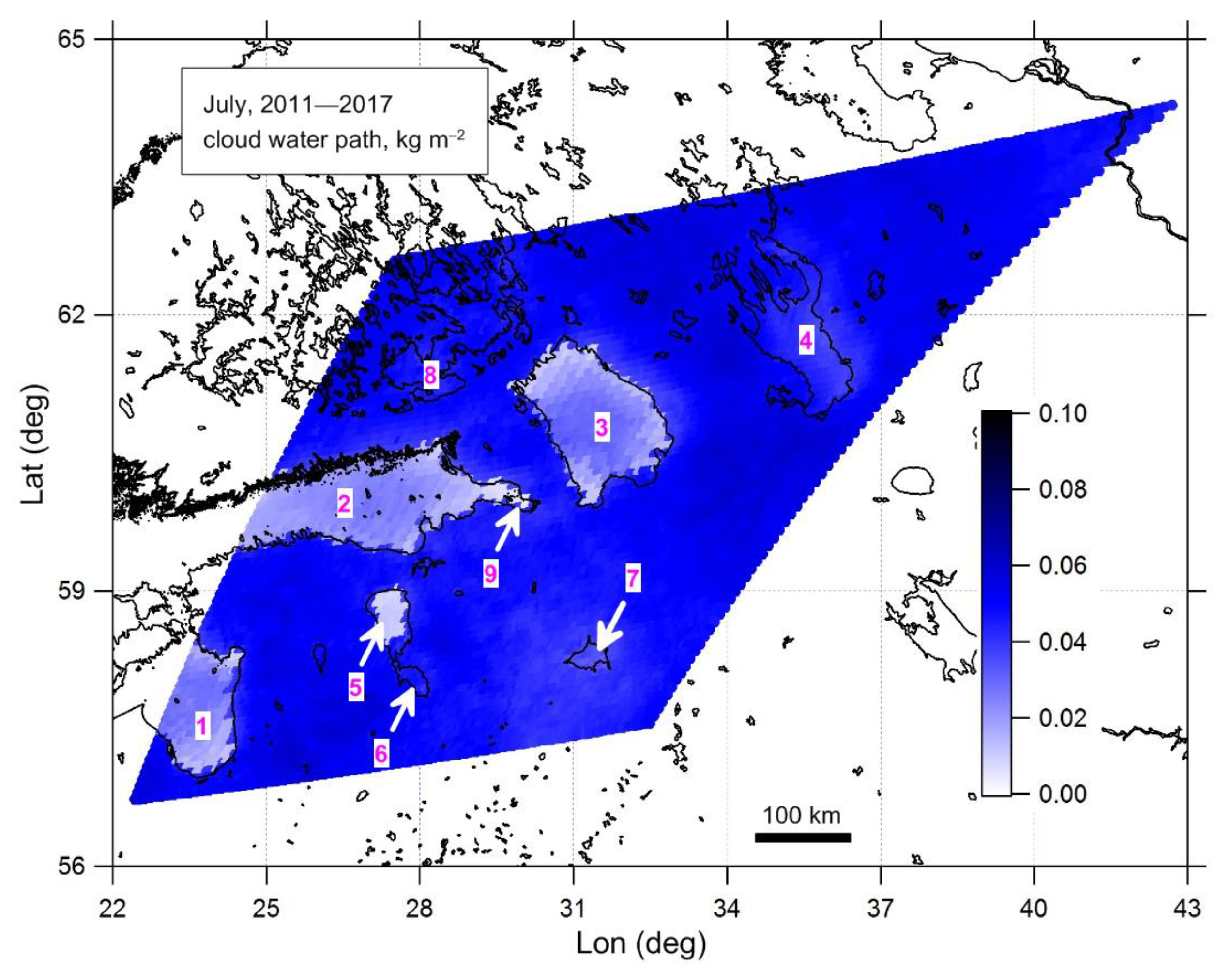
Figure 1 shows the geographical domain and the water bodies under investigation. As an example, the map of the mean LWP values for July averaged over all 7 years of observations (2011–2017) is also shown (the colour scale represents the LWP in kg m⁻²): one can see that the LWP land-sea differences exist for all considered water bodies. Despite the fact that lakes Peipus and Pihkva are located near each other and are connected, we consider them separately since the area of Lake Pihkva is about three times smaller than the area of Lake Peipus. The present study contains an analysis of the LWP contrast values at several specific locations in the vicinity of the water bodies enumerated in Figure 1. These locations (pairs of the SEVIRI ground pixels) were selected to a certain extent arbitrarily, but we tried to consider the following two cases: the land and the sea pixels of the satellite measurements are far from a coastline and the distance between them is large (case 1), and they are near a coastline with small distance between them (case 2). For cases 1 and 2, the distances between each of the two measurement locations and the coastline are about 40 km and 10 km, respectively. Thus, the total distance between measurement locations is about 80 km (case 1) and 20 km (case 2). In addition, we tried to select the land and sea pixels in such a way that the line that connects them is oriented close to the south-north direction. The reason for that was our intention to avoid the influence of the effect of the cold air transport by westerly winds from the water bodies to the land. The westerly and south-westerly winds are predominant in the area of the Gulf of Finland [26]. The geographical coordinates of the selected pixels are presented in

Table 1. Geographical coordinates, the total number of LWP measurements selected for analysis, and the data set designation.

Water Body	Data Set	Coordinates of Measurement Locations		Total Number of Measurements		Distance between Pixels
		Sea	Land	Warm Season (June–August)	Cold Season (February–March)
1. The Gulf of Riga	ML1-1	57.366416 N, 23.664965 E	56.765244 N, 22.910569 E	15,924	4655	LD **
	ML1-2	57.139038 N, 23.385504 E	56.993382 N, 23.193808 E	17,884	5065	SD ***
2. The Gulf of Finland	ML2-1	59.857132 N, 25.299348 E	59.144346 N, 25.536151 E	15,478	3824	LD
	ML2-2	59.583547 N, 25.387536 E	59.404679 N, 25.452862 E	17,139	4196	SD
3. Lake Ladoga	ML3-1	60.487217 N, 32.255603 E	59.787115 N, 32.622665 E	16,277	3596	LD
	ML3-2	60.228835 N, 32.387668 E	60.056733 N, 32.484774 E	17,169	3704	SD
4. Lake Onega	ML4-1	61.389299 N, 35.810093 E	60.726050 N, 36.389155 E	15,034	2934	LD
	ML4-2	61.147303 N, 36.018435 E	60.978995 N, 36.167049 E	15,874	2679	SD
5. Lake Peipus	ML5	58.906952 N, 27.367954 E	59.091926 N, 27.350632 E	16,457	4040	SD
6. Lake Pihkva	ML6	57.940914 N, 27.992420 E	57.763346 N, 27.942981 E	17,305	4532	SD
7. Lake Ilmen	ML7	58.235672 N, 31.173657 E	58.058871 N, 31.117336 E	18,006	4454	SD
8. Lake Saimaa	ML8	61.222858 N, 28.439451 E	61.042522 N, 28.468290 E	16,421	3662	SD
9. The Neva River Bay *	ML9	59.957250 N, 29.913798 E	59.880953 N, 29.826097 E	18,001	4282	SD

* Corresponds to ground-based microwave measurements from the study by Kostsov et al. [5]. ** large distance (about 80 km, see text). *** small distance (about 20 km, see text).

and

Table 2. Same as Table 1 but for additional measurement locations.

Water Body	Data Set	Coordinates of Measurement Locations		Total Number of Measurements		Distance between Pixels
		Sea	Land	Warm Season (June–August)	Cold Season (February–March)
10. The Gulf of Finland, Kalvi	ML10	59.580558 N, 26.846173 E	59.407040 N, 26.723764 E	17,279	4370	SD
11. The Narva River Bay	ML11	59.490327 N, 27.810318 E	59.308683 N, 27.811472 E	16,931	4460	SD
12. The Luga River Bay	ML12	59.766497 N, 28.324202 E	59.586924 N, 28.325356 E	17,588	4312	SD
13. The Gulf of Finland, Helsinki	ML13	60.167451 N, 25.310649 E	60.341055 N, 25.226349 E	17,146	4059	SD
14. The Gulf of Finland, Torfyanovka	ML14	60.428589 N, 27.962023 E	60.609377 N, 27.918291 E	16,996	3938	SD

together with other characteristics of the data sets. The data sets are named as ML with one or two numbers. ML stands for “measurement location.” The first number identifies the location, and the second number identifies large (1) or small (2) distance between pixels, if applicable. Table 2 presents additional measurement locations that have been selected in the course of the analysis to investigate the Gulf of Finland in more detail (see subsequent sections of the article). The locations that have been selected for analysis are shown in Figure 2 on the domain map.

The data selection algorithm was applied sequentially for all measurements during 2011–2017 and included checking of the quality flag, solar zenith angle, and the cloud phase. It should be noted once again that clear sky cases were included in the data sets as well. For the mentioned specific locations, all data selection criteria should have been satisfied simultaneously for the land pixel measurement and the sea pixel measurement, which correspond to a single SEVIRI scan; if not, both the land and sea measurements were filtered out. Finally, we have at our disposal the good quality data on LWP corresponding only to liquid phase clouds and clear sky cases and acquired when the solar zenith angle was smaller than 72°. In order to reveal the principal features of the LWP contrast, in this study, we limited the analysis by taking into consideration only two time periods. The first period consists of three summer months, and the second period includes February and March. The choice of the summer months is evident, but the choice of February and March needs some explanation. Since we explore Northern latitudes, the solar zenith angle is very large during winter, resulting in a very small number of SEVIRI measurements suitable for analysis. Such measurements are completely absent in December and January. There are only a few measurements in February. Luckily, March is well applicable for analysis due to sufficiently small solar zenith angle values, and at the same time, it can be considered as a winter month since during March, usually, the land is still covered by snow and water bodies are still covered by ice in the region of our interest. When a cold season is characterised by anomalously high air temperatures, this assumption may not be valid. Taking into account the possibility of such situations, one can conclude that there might be problems with retrievals (potential biases) that are caused by different surface reflectance and consequently by misclassifications during application of the cloud mask, the sea-ice mask, and the snow mask. A good illustration of the problems of that kind can be found in the study by Kostsov et al. [4]. This study has revealed the abnormal LWP land-sea contrast (very high LWP values over water) in the data from the satellite instrument AVHRR over several water bodies of moderate and small size in Northern Europe during the cold season of 2013, while during the cold season of 2014, such an effect was not detected. It is important to have in mind that in 2013, these water bodies were covered by ice, while in 2014, they were ice-free due to abnormally high air temperature. The analysis has shown that there were probably problems with the sea-ice and snow masks in 2013, and the high reflectance of ice and snow in combination with the large viewing angle of the AVHRR instrument resulted in erroneous high values of LWP during clear-sky conditions. That is why AVHRR produced unexpected very high abnormal land-sea LWP contrast. The spring season in 2014 started early, and the snow and ice cover disappeared quickly. Due to the absence of the reflectance from ice and snow, the AVHRR measurements reported correct values of LWP. We would like to emphasise the complexity of the problem by noting that neither in 2013 nor in 2014 were there erroneous data from AVHRR over the large Lake Ladoga, which was covered by ice in 2013 and also in 2014 despite the warm and early spring of 2014. Thus, the problems may also arise due to disagreement of the size of a water body and the spatial resolution of masks that are used in the retrieval algorithms. Taking into account this example, one can conclude that rigorous consideration of the state of the underlying surface in the analysis can be done only for a specific location and only together with the information on the applied cloud/land/water/ice/snow mask. Since we have no such information at our disposal and consider a large variety of water objects, we do not split the data into any groups depending on the surface state, but we keep in mind that the data for the cold seasons might have larger errors than for the warm season.

Table 1 presents the total number of selected measurements within the two mentioned time periods. One can see that for all the measurement locations, the number of selected measurements during the warm season is large and considerably exceeds the number of measurements during the cold season. The data sets for Lake Onega contain the smallest amount of data for the cold season, which is, however, sufficient for the statistical analysis.

In order to identify possible data gaps that may influence the results of the analysis, we calculated for each month the percentage of days P_d with good quality data, which were used for the analysis. These calculations have shown that for June, July, and August (the warm season) and for March (the cold season) and all years of observations, there are no data gaps, and there are no noticeable inter-annual variations of P_d for all locations. In addition, there is no noticeable difference between the P_d values for different locations: they are mostly within the interval 80–100%. For February (cold season), the P_d values considerably differ from location to location within the interval 10–70%, but for a single location, the inter-annual difference is not considerable.

3. Seasonal and Inter-Annual Features of the LWP Land-Sea Contrast

Figure 3 presents typical statistical distributions of the LWP land-sea contrast for specific measurement locations for the warm season and for the cold season (all years together). The central peak of the distributions corresponds to zero value of the LWP contrast. This peak is very sharp in all plots; therefore, for better visibility, the vertical axes are broken and have different scales in the lower and upper parts. It is obvious that if the prevailing positive or negative LWP difference exists, it will show up as the asymmetry of a distribution. One can see such asymmetry in Figure 3 for measurement location ML1 (the Gulf of Riga) for both seasons. Both negative and positive values of the contrast are present in the distributions for ML1; however, positive values of contrast have the higher frequency of occurrence in all cases. The distributions similar to ML1 are detected for ML2 (the Gulf of Finland).

Opposite to the distributions for the Gulf of Riga (Figure 3a,b), the statistical distributions of the LWP difference for Lake Onega are almost symmetrical (Figure 3c,d). A similar symmetrical distribution is detected for Lake Ladoga in a cold season (not shown). However, in a warm season, a large-distance contrast ML3-1 at Lake Ladoga is characterised by an asymmetrical distribution similar to the one shown in Figure 3a,b. This result is to some extent unexpected, taking into account the fact that both Lake Ladoga and Lake Onega are featured by low temperature of water in summer, so the land-sea contrast of the near-surface temperature is expected to be noticeable for both of these lakes. In addition, attention should be paid to the shape of symmetrical distributions for the cold season: an extremely sharp central peak at the zero value and more or less uniform distributions of negative and positive values with a very small frequency of occurrence. The distributions for the locations M6, M7, and M8 are not shown. They are similar to each other in shape both for warm and cold seasons and demonstrate very small asymmetry, however with prevailing positive values, as those in Figure 3c,d.

Figure 3e,f shows the LWP contrast distributions for measurement locations ML5 (Lake Peipus) and ML9 (the Neva River Bay) which are characterised by very pronounced asymmetries. One can see that the negative contrasts are almost completely absent for both seasons. For ML9, the very small negative values of the land-sea contrast can be seen only for the warm season. Thus, in addition to the distributions, which we can designate as “type 1” and “type 2” and which are shown in Figure 3a,b and Figure 3c,d correspondingly, we have the “type 3” distribution, which is characterised by the absence of negative contrasts. Distributions of type 3 are quite unexpected. The ground pixel size of measurements is about 7 km. The detected LWP value is an approximation of the mean LWP for all clouds within the pixel. In the case of a broken cloud field, the distribution of separate clouds within the land pixel and sea pixel can be obviously considered as random. As a result, statistically, the situations with negative LWP contrast must be present, and their frequency of occurrence must not be negligibly small due to the fact that the cloud fields have very high spatial and temporal variability. At the moment, we cannot find any natural reason for the existence of LWP contrast distributions of type 3. It should be emphasised that type 3 distributions have been detected only for two locations, ML5 and ML9. One can suggest that they reflect some artefact that manifests only for these two water bodies of medium size. Further research is needed, which should be based on a considerably larger number of specific measurement locations.

To get more insight into the features of the LWP land-sea difference, we plotted the inter-annual variations of the seasonal mean LWP difference for a number of locations, see Figure 4 and Figure 5. First of all, we pay attention to the standard error of the seasonal mean values (SESM) for cold and warm seasons. The values of SESM are calculated by dividing the standard deviation by the square root of the sample size. SESM is a measure that shows how accurately the mean value obtained from the set of samples represents the true mean value of the entire distribution. In other words, it characterises how representative our data sets are. We would like to note that we use the a priori assumption of uncorrelated measurements and of the absence of systematic errors in the LWP data from SEVIRI. In addition, we assume that all meteorological situations typical for specific season or month are implicitly present in each of the corresponding data sets. For better visibility, we did not plot the error bars together with the curves except for in one case: to give an impression of the magnitude of the error of the mean difference, in Figure 5c,d, we show the error bars for the results corresponding to ML9. The errors during the cold season can reach 0.004 kg m⁻². The errors for the warm season constitute about 0.001–0.002 kg m⁻².

Analysis of Figure 4 and Figure 5 leads to the following conclusions:

• The inter-annual variability of the LWP seasonal mean land-sea contrast is considerably different for the cold season and the warm season. The contrast is highly variable for the cold season, while for the warm season, in many of the considered cases, it is close to a constant value.
• For all considered years, the LWP land-sea difference during the warm season is always positive, while the situation changes for the cold season. Negative values of the difference are detected for cold seasons of several years at measurement locations ML3, ML4, ML6, ML7, and ML8. We emphasise that the negative difference was detected at ML2 only once during the cold season of 2013, and its absolute value was negligibly small.
• If we consider the warm season, we can easily classify the LWP difference values as belonging to three groups: small values (ML3-2, ML4, ML6, ML7, ML8), moderate values (ML1, ML2, ML3-1), and large values (ML5, ML9).
• The locations ML5 and ML9 are very specific: large positive differences are detected during both cold and warm seasons.

4. Intra-Seasonal Features of the LWP Contrast

Since the amount of data acquired during the cold season is smaller than during the warm season and almost all data refer to only one month (March), we analysed the intra-seasonal variability of the LWP land-sea contrast only for the warm season. Figure 6 demonstrates the daily mean values of the LWP contrast in June, July, and August for all seven years of observations. The most robust evidence of the time dependency of the LWP contrast is present at three measurement locations: ML1-2 (shown in Figure 6a), ML9 (shown in Figure 6b), and ML2-2 (not shown, the same as for ML1-2). One can see that in June and July, large and moderate positive values of the LWP contrast are prevailing, while in August, the values are much smaller (in terms of absolute values), and positive and negative differences occur with equal frequency. The common feature of two locations ML1-2 and ML-9 is that they are in the vicinity of the estuary of rivers: Western Dvina (Daugava) for ML1-2 and Neva for ML9. The common feature of all three locations (ML1-2, ML2-2, and ML9) is that they correspond to the small-distance LWP difference, and all of them are situated in the gulfs of the Baltic Sea.

The absence of any noticeable time dependence of the LWP contrast during the warm season at other locations is illustrated by Figure 6c,d. To save space, only two locations are shown, which represent large differences (ML5) and very small differences (ML6). The results for ML7 and ML8 are similar to the results for ML6. The results for ML3-2, ML4-1, and ML4-2 are similar to the results for ML5. In order to get a more precise estimation of the time dependence rather than demonstrative plots, we present the diagrams of the monthly mean values of the LWP land-sea differences for the whole 7-year period in Figure 7. Colours in Figure 7 are used to designate three groups of water bodies: gulfs of the Baltic Sea, large lakes, and small lakes. Figure 7 demonstrates once again that there are three locations that are characterised by very small differences in August if compared to June and July: ML1-2, ML2-2, and ML9. The locations ML1-1 and ML2-1 may also be attributed to this group; however, for these locations, the LWP land-sea difference in August is higher than for ML1-2, ML2-2, and ML9. One can also notice that there is another characteristic feature of the intra-seasonal behaviour of the LWP land-sea contrast: maximum values are detected in July in most cases (ML1-1, ML1-2, ML2-1, ML3-1, ML4-1, and ML8). No definite time dependence is detected for ML5, ML6, ML7, ML3-2, and ML4-2 (small lakes and small-distance LWP difference at large lakes).

One can see that all measurement locations with small LWP contrast in August are situated in the Baltic Sea. In order to study this phenomenon in more detail, we selected five more locations in the Gulf of Finland. All these additional locations correspond to a short-distance LWP difference and are described in Table 2. Two of them (ML11 and ML12) are close to estuaries of the rivers Narva and Luga. ML10 is situated in between ML2-1 and ML11. Two of the five additional locations are at the Northern coast of the Gulf of Finland (near Helsinki and Torfyanovka). The intra-seasonal variability of the monthly mean LWP land-sea contrast averaged over the 7-year period for these additional locations is shown in Figure 8. One can see that for all additional measurement locations, the time dependence of the LWP contrast is the same as for the main locations at the coastline of the Gulf of Finland. One can also see that there are no features that would in one way or another distinguish the contrast obtained near the estuaries of rivers or at the northern coastline with respect to the contrast at other locations.

For convenience, the revealed effect will be referred to below as the “August anomaly.” The similarity of results obtained for different locations in the Baltic Sea can lead to a conclusion about possible common physical mechanisms that drive the LWP land-sea difference in the entire Baltic Sea region considered in the present study. However, now we are coming around to the opinion that the “August anomaly” is an artefact of the SEVIRI measurements. The arguments in favour of this hypothesis are, first of all, the immediacy of the transition from large LWP contrast to very low contrast (just within a couple of days) and, second, the fact that this transition occurs exactly at the end of July—beginning of August at all examined locations in the Gulf of Finland and the Gulf of Riga. This fact is illustrated in Figure 9, where the daily mean values of the LWP contrast for all locations in the Gulf of Finland and the Gulf of Riga are shown. Averaging of daily mean values was done over all seven years of observations. Running averaging over 3 days was used only for better visibility of the results. It is unlikely that natural meteorological processes change so sharply, synchronically, and at the same date every year at different places in the Baltic Sea. Thus, we assume that the “August anomaly” can be an artefact that reflects certain algorithmic features in the SEVIRI data.

5. Comparison with the Reanalysis Data

It is interesting and important to compare the obtained statistical characteristics of the LWP land-sea difference with the data provided by reanalyses. Wright et al. [28] note that although cloud fields in reanalyses are essentially model products, many variables that influence the cloud fields are altered during the assimilation process. Therefore, detecting differences between the LWP contrast values obtained in experiments and those provided by reanalyses can be valuable for identification of possible problems in reanalyses and for future model development. Li et al. [29] have noted that “reanalysis products have become nearly synonymous, in some contexts, with ‘observations’” and they pointed out the necessity “to provide some assessment of this tenuous perception—particularly for quantities such as CLWP and CLWC” (here, CLWP and CLWC stand for cloud liquid water path and cloud liquid water content, respectively).

In the present study, we consider the ERA-Interim and ERA5 reanalyses from ECMWF (European Centre for Medium-Range Weather Forecasts), see for details the papers [6,30]. The main shortcoming of the comparison of the reanalysis data with the experimental values of the LWP land-sea contrast is the coarse spatial resolution of the reanalysis data: the internal resolution of ERA-Interim is 0.75°, which is about 80 km. For higher resolutions of the ERA-Interim data, an interpolation procedure is applied, but the highest recommended resolution is 0.25° (28 km). In the present study we have chosen the 28 km resolution of ERA-Interim, and in this case, we can compare the ERA-Interim data with the SEVIRI results, which correspond to the long-distance LWP difference. If compared to ERA-Interim, the ERA5 reanalysis has a considerably higher standard resolution of 31 km, and it also has a higher temporal resolution (1 h versus 6 h in ERA-Interim). Besides, there are other improvements in ERA5. We compare the experimental values of the LWP land-sea contrast with both reanalyses, ERA-Interim and ERA5. A map showing the geographical locations of the reanalysis grid points used for calculations of the LWP land-sea difference is presented in Figure 10. These locations are designated similarly to the corresponding SEVIRI measurement locations: RE1-1, RE2-1, RE3-1, and RE4-1, where RE stands for reanalysis. It should be noted that grid boxes of ERA5 have been selected in a way to be fully placed over sea or land. Such selection was possible since long distance LWP differences are considered. In addition, one should keep in mind that for ERA-Interim, due to coarser original spatial resolution, the original grid boxes (before interpolation to a 28 km grid) can contain a small portion of the “wrong” surface: sea for a land grid box and land for a sea grid box.

There were three options for how to organise all three data sets with respect to temporal sampling. The first evident variant was to select the synchronous data corresponding to 6 h and 12 h UTC from ERA-Interim, ERA5, and SEVIRI. The second choice was to synchronise the data from reanalyses only (for 6 h and 12 H UTC) and to use the entire SEVIRI data set. And the third option was to use the original time sampling for each data set. We emphasise that only the daytime data are considered. We selected the third option for three main reasons. First of all, our goal was to compare the averaged daytime values for reasonably long time periods; therefore, we tried to keep as much initial data as possible. This is especially important for a cold season and SEVIRI data. Second, we did not intend to compare the two versions of reanalysis but rather wanted to show the agreement or disagreement of reanalyses with the satellite data. In this respect, it was important to keep all improvements that are present in ERA5, in particular its high temporal resolution. The last but not the least reason is that in our previous study [5], we used the original temporal resolutions when we compared averaged LWP from three data sets: ERA-Interim, SEVIRI, and ground-based microwave observations. In order to be consistent with the illumination conditions of the SEVIRI observations, in the present study, the reanalysis data on LWP corresponding to solar zenith angle larger than 72° were filtered out. It is important to note that the data selected from reanalyses contained the clear-sky cases and the cases with liquid clouds only, and in this respect, all data sets were completely consistent.

Figure 11 presents the examples of statistical distributions of the LWP contrast at the location RE2-1 obtained from the ERA-Interim and the ERA5 data. These distributions are typical for all four locations that have been selected for collecting the reanalysis data. One can see that the distributions are asymmetrical for the warm season and symmetrical for the cold season. For the warm season, the distributions derived from reanalysis are similar to the distributions with moderate asymmetry obtained from the SEVIRI data, but the central peak is not so sharp. For the cold season, the statistical distributions from reanalysis differ noticeably from distributions derived from the SEVIRI data: there is no pronounced central peak, and the wings are not as flat as they are for the SEVIRI distributions. Highly asymmetrical distributions without negative LWP land-sea contrast revealed from the SEVIRI data are absent in reanalysis.

The comparison of the seasonal mean LWP contrast from SEVIRI with the data from ECMWF reanalyses is presented in Figure 12 for the period 2011–2017. The most important conclusion that can be derived from this comparison is that the magnitude of the LWP contrast provided by the ERA5 reanalysis is much larger than that provided by ERA-Interim. It should be emphasised that this discrepancy between the two reanalyses is clearly seen for both cold and warm seasons. Moreover, while ERA-Interim shows small positive and negative values of the LWP difference during the cold season, the values from ERA5 during the cold season are predominantly positive, and this fact is rather important. For three locations (ML1-1, ML2-1, and ML3-1), the agreement between SEVIRI and ERA5 is much better than between SEVIRI and ERA-Interim. For the case with ML2-1, the agreement between the ERA5 and SEVIRI data can even be characterised as very good since the inter-annual behaviour is quantitatively and qualitatively similar. However, attention should be paid to the fact that for all locations, ERA5 systematically overestimates the LWP contrast from SEVIRI during the warm season. At the same time, ERA-Interim underestimates the LWP contrast from SEVIRI during the warm season with only one exception at location ML4-1 (Lake Onega): the magnitudes of the SEVIRI and the ERA-Interim reanalysis data are in good agreement here.

Figure 13 presents the intra-seasonal variability of the LWP land-sea contrast in terms of the monthly mean (June, July, and August) values derived from the SEVIRI data and from the ERA-Interim and ERA5 reanalyses. First of all, we pay attention to the fact that the ERA-Interim results show the feature that looks similar to the August anomaly revealed by SEVIRI: the LWP contrast in August is noticeably smaller than in June and July at a large number of locations (see Section 4). Contrarily, ERA5 shows another type of the intra-seasonal variability: the LWP contrast values in June and August are comparable with each other, and at the same time, they are smaller than the LWP difference for July. None of the reanalyses demonstrate similar qualitative or quantitative behaviour for the considered locations. It is important to note that for all locations and months, ERA5 overestimates the LWP differences if compared to the SEVIRI data. Rather, ERA-Interim strongly underestimates the experimental data, except for location ML4-1. On the whole, the ERA5 reanalysis seems to have advantages with respect to the ERA-Interim reanalysis.

Finally, we show Figure 14, which demonstrates that ERA-Interim does not reproduce the August anomaly of the SEVIRI data despite the fact that the LWP contrast obtained from ERA-Interim in August is much lower than the contrast in June and July. Figure 14 presents intra-seasonal (June–August) variability of the daily mean LWP land-sea contrast obtained from the ERA5 and ERA-Interim reanalysis for locations RE1-1 and RE4-1. For these two locations, the monthly mean values of the LWP contrast in August from ERA-Interim are the lowest with respect to June and July, as it is shown in Figure 13. One can see from panels (b) and (d) in Figure 14 that two characteristic features of the August anomaly revealed by SEVIRI are absent. In the ERA-Interim data, in June and July, both positive and negative contrast values are present. Moreover, there is no considerable difference between the absolute values of the contrast in June–July and August. However, these features are clearly seen in the SEVIRI data shown in Figure 6a,b. Moreover, one cannot see any noticeable difference between the results from ERA-Interim and ERA5 except the fact that positive contrast values are predominant in the ERA5 data.

6. Summary and Conclusions

Studying interactions between different components of the climate system (the atmosphere, the hydrosphere, and the land surface) is a very interesting scientific task due to the involvement of many processes of different kinds in these interactions. Cloud liquid water path (LWP) is the quantity that can be an indicator of some of these processes, relevant, in particular, to an exchange of moisture and heat between a surface and the atmosphere. Understanding the distribution of LWP over land, water, and coastal zones is crucial for determining the radiation budget in these areas. Clouds reflect solar radiation and absorb longwave radiation emitted by the earth’s surface, affecting in this way the energy budget and evaporation. Clouds can be not only an indicator of mesoscale circulation, which is characterised in coastal zones by breezes and background winds, but also an active element of the circulation processes due to much feedback. The goal of the present study is to analyse the phenomenon of the LWP horizontal inhomogeneities in the vicinity of various water bodies in Northern Europe (so-called the LWP land-sea contrast) detected from the space-borne observations by the SEVIRI instrument in 2011–2017. Focus is on the temporal and spatial variation of LWP.

The data selected for analysis refer to the liquid cloud phase only; ice and mixed-phase cloud cases were filtered out. These data comprise all cases including clear sky over land and water surfaces that occurred simultaneously and not simultaneously as well. It should be emphasised that the data refer to the daytime only because the LWP retrieval method is based on the measurements of reflected solar radiance. The objects of investigation are water bodies in Northern Europe that differ in size and geomorphology: the Gulf of Finland, the Gulf of Riga, the Neva River Bay, and lakes Ladoga, Onega, Peipus, Pihkva, Ilmen, and Saimaa. Two types of the LWP land-sea contrast have been considered: the short-distance contrast and the long-distance contrast (20 km and 80 km between land and sea measurement pixels, respectively).

The statistical distributions and the values of the LWP land-sea contrast averaged over a large number of measurements have been used for analysis. The analysis has shown the following:

• The statistical distributions of the LWP land-sea contrast vary from symmetrical ones with the pronounced peak at zero value and Gaussian-shaped slopes to strongly asymmetrical ones without negative values. These strongly asymmetrical distributions without negative values can be artefacts that appear for specific water bodies and measurement locations.
• The inter-annual variability of the LWP seasonal mean land-sea contrast is considerably different for cold and warm seasons. The LWP difference is highly variable for the cold season, while for the warm season in many of the considered cases, it is close to a constant value. For all analysed years, the contrast during the warm season is always positive, while the situation is different for the cold season.
• The maximal values of the LWP contrast are observed in the vicinity of the Neva River Bay and of Lake Peipus.
• The intra-seasonal variability of the LWP land-sea contrast has been analysed only for a warm season because of lack of data for a cold season. It has been found that in the Gulf of Riga and the Gulf of Finland of the Baltic Sea in June and July, large and moderate positive LWP differences are prevailing, while in August, positive and negative differences are much smaller (in terms of absolute values) and occur with equal frequency. This phenomenon can be called “the August anomaly.” The transition from large LWP contrast to very low contrast occurs abruptly just within a couple of days exactly in the beginning of August. Obviously, it is unlikely that natural meteorological processes change so sharply, synchronically, and at a certain date every year at different places in the Baltic Sea. Thus, we assume that the “August anomaly” can be an artefact that reflects certain algorithmic features in the SEVIRI data.

The obtained statistical characteristics of the LWP land-sea difference have been compared with the data provided by reanalyses ERA-Interim and ERA5 from ECMWF. Because of the coarse spatial resolution of the reanalysis data, the comparison has been made for four locations only and for the long-distance LWP land-sea difference (the Gulf of Riga, the Gulf of Finland, lakes Ladoga and Onega). The analysis has shown the following:

• For the warm season, the distributions derived from reanalysis are similar to the distributions with moderate asymmetry obtained from the SEVIRI data, but the central peak is not so sharp. Highly asymmetrical distributions without negative LWP land-sea contrast revealed from the SEVIRI data for a few locations are absent in reanalysis.
• The magnitude of the LWP contrast provided by the ERA5 reanalysis is much larger than that provided by ERA-Interim. It should be emphasised that this discrepancy between two reanalyses is clearly seen for both cold and warm seasons. ERA-Interim predominantly underestimates the LWP differences from SEVIRI for considered water bodies during the warm season and provides negative differences during the cold season. The ERA5 reanalysis data are in better qualitative and quantitative agreement with the satellite data despite the fact that they systematically overestimate the experimental data during the warm season.
• The ERA5 data provide no indication at all of the existence of the “August anomaly” in the gulfs of the Baltic Sea. The ERA-Interim results show a feature that looks similar to the August anomaly for the Gulf of Riga and Lake Onega: the LWP contrast in August is noticeably smaller than in June and July. However, two characteristic features of the August anomaly revealed by SEVIRI are absent. In the ERA-Interim data, in June and July, both positive and negative contrast values are present. In addition, there is no considerable difference between the absolute values of the contrast in June–July and August. However, these features are clearly seen in the SEVIRI data. Thus, the analysis has shown that ERA-Interim also does not provide any confirmation of the “August anomaly”.

The present study has demonstrated large variability of the features of the LWP land-sea contrast for different locations, especially for lakes, and these features, as we believe, require further investigation. Some features (strongly asymmetrical statistical distributions for some locations, the “August anomaly” in the gulfs of the Baltic Sea, very high values of the contrast detected for only two locations at Lake Pihkva and the Neva River Bay) seem to be artefacts rather than of natural origin. It should be noted that the effect of an abrupt and large change of the LWP contrast value referred above as the “August anomaly” may be present not only in summer but also at other times beyond the time periods taken for analysis in the present work. Thus, although this research does not provide a definite answer to the question posed in the article title, it can be seen as a first attempt to explore in detail the spatial and temporal variability of the LWP land-sea contrast in the vicinity of various water bodies in Northern Europe. Finally, we would like to note that the approach to studying the LWP land-sea contrast that we have demonstrated can be applied to the LWP data from the AVHRR instrument, which has much in common with the SEVIRI instrument regarding the physical principle and methodology of the LWP retrieval.