A Survey of Automotive Radar and Lidar Signal Processing and Architectures

Abstract

In recent years, the development of Advanced Driver-Assistance Systems (ADASs) is driving the need for more reliable and precise on-vehicle sensing. Radar and lidar are crucial in this framework, since they allow sensing of vehicle’s surroundings. In such a scenario, it is necessary to master these sensing systems, and knowing their similarities and differences is important. Due to ADAS’s intrinsic real-time performance requirements, it is almost mandatory to be aware of the processing algorithms required by radar and lidar to understand what can be optimized and what actions can be taken to approach the real-time requirement. This review aims to present state-of-the-art radar and lidar technology, mainly focusing on modulation schemes and imaging systems, highlighting their weaknesses and strengths. Then, an overview of the sensor data processing algorithms is provided, with some considerations on what type of algorithms can be accelerated in hardware, pointing to some implementations from the literature. In conclusion, the basic concepts of sensor fusion are presented, and a comparison between radar and lidar is performed.

1. Introduction

In recent years, Advanced Driver-Assistance Systems (ADASs) have performed many steps forward, making autonomous driving a reality. Going toward full driving automation (

Table 1. ADAS levels and related automation level.

ADAS Level	Automation Level
Level 0	No Automation
Level 1	Driver Assistance
Level 2	Semi-Automated
Level 3	Conditional Automation
Level 4	High Automation
Level 5	Full Automation

), it is necessary to study sensors and acquisition systems that guarantee proper performance, mainly in terms of accuracy and resolution.

Nowadays, the most promising sensor systems to support the development of ADASs are based on radar and lidar. Both permit detection and ranging but, while the former exploits radio-frequency (RF) signals, the latter exploits optical signals. The debate on which one will be the genuinely enabling technology for autonomous driving is still open. In fact, many of the solutions that are available on the market adopt either radar, lidar or a combination of them.

Automotive applications of radar are well known, and have been highlighted during the last fifty years. An overview of the status during its first years can be found in [1]. Many review articles have presented automotive radar focusing on the related signal processing algorithms [2] or the required hardware technology [3]. More recent works report and discuss signal processing, modulation aspects and higher-level processing, such as tracking and classification [4,5].

Lidar’s first applications were far from the automotive world, but today, this detection technique has become essential to develop ADASs and autonomous driving features. An overview of the principal modulation schemes and integration techniques can be found in [6], with a particular remark on electronic-photonic integration. An overview of the imaging systems with some technological information is available in [7]. Some recent reviews highlight how lidar data processing is mainly based on machine learning [8,9,10]. Li et al. [11] give an overview of how to use lidar as a detection system, and gives an overview of the detection and recognition algorithms. In recent years, lidar systems are available as plug and play detection systems, so Roriz et al. [12] give an overview of the devices available on the market. More recently, Bilik et al. [13] give a comparative overview of the radar and lidar systems, which focuses on differences and similarities of these two systems.

This review mainly presents an overview of state-of-the-art radar and lidar algorithms and architectures. Then, the concept of sensor fusion is briefly outlined, and some architectures are shown as examples of hardware acceleration of radar- and lidar-related computation. In conclusion, a short comparative analysis is reported to highlight differences and similarities of lidar and radar.

2. Radar

At the beginning of the 20th century, radio detection and ranging (radar) systems were proposed to detect and locate aircraft [14]. With the consolidation of technology and its availability at a relatively low cost, many different application domains have been found for radar systems. Nowadays, radar represents a well-established technology in the automotive industry [1].

Applications of radar systems on vehicles are numerous and extensive, mainly related to tasks in which the distance to a target vehicle and its relative velocity have to be measured, e.g., the autonomous emergency braking (AEB) and adaptive cruise control (ACC) systems [15].

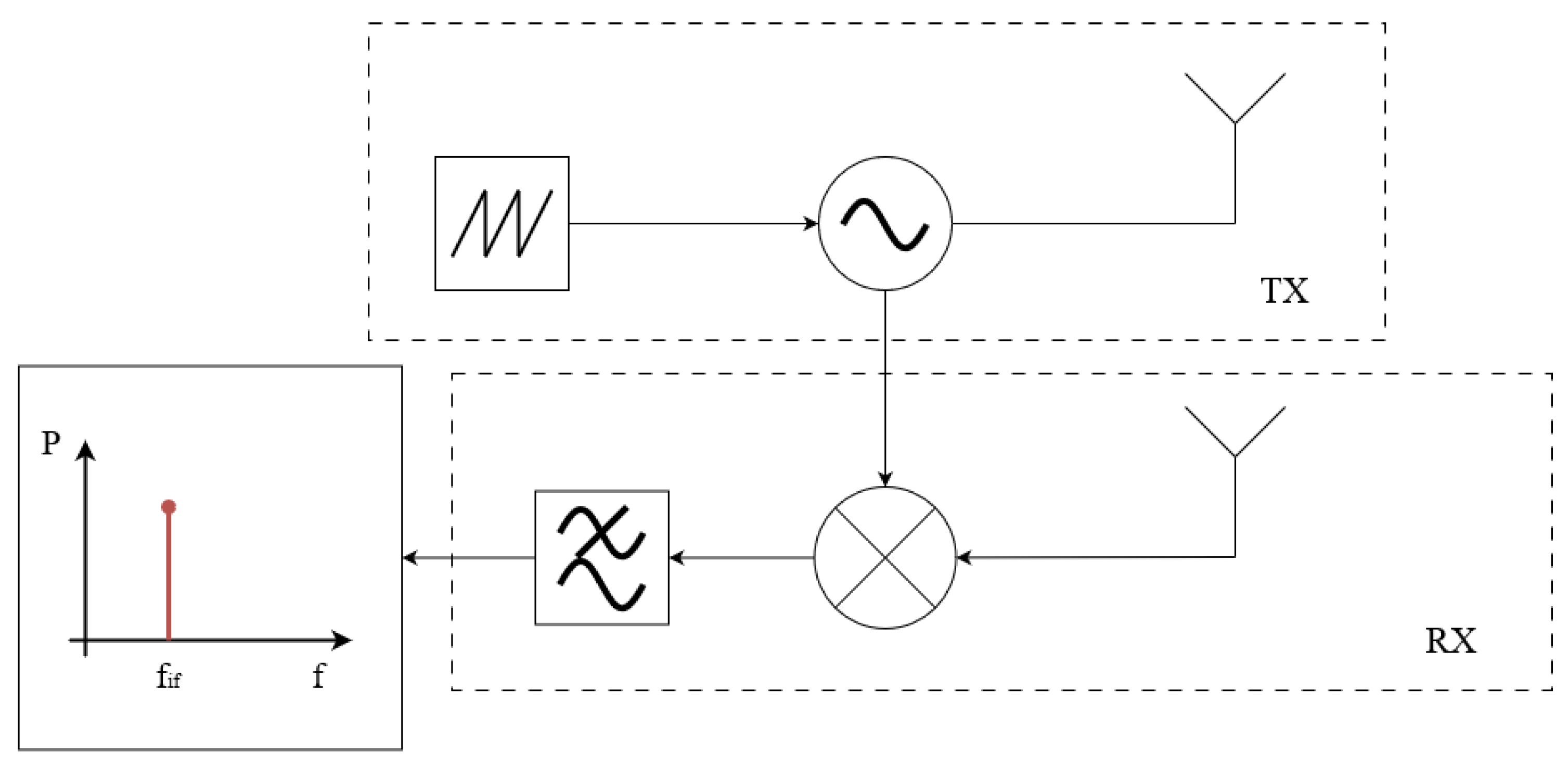
2.1. Operating Principles

The basic idea behind radar is to send a radio-frequency signal in free space and collect the echo generated by the presence of an obstacle. It is possible to determine the distance to the reflecting object by measuring the delay between the transmitted and the received signals. Figure 1 shows a conceptual example of how a radar system works. Equation (1) permits us to calculate the distance d of an object by measuring $\tau$, the delay of the received signal, and c, the speed of light in the air [16]:

$$d=\frac{1}{2}c\tau ,$$

(1)

Even if the main idea remained substantially unchanged, many algorithms and systems have been developed during the last years to increase performance and resolution of radar systems.

The following sections present and analyze the main architectures and algorithms available nowadays for automotive radars.

2.2. Radar Technology and Modulations

The primary accepted and most widespread technology for radar systems relies on frequency-modulated continuous wave (FMCW) signals [17].

The key idea is to send a sequence of analog chirps; then, the transmitted signal is mixed with the received one, and the resulting beat frequency will be proportional to the target distance.

Figure 2 reports the basic scheme of an FMCW radar. In particular, on the transmitter side (TX in Figure 2), the saw-tooth waveform generator produces a wave that then feeds a voltage-controlled oscillator producing a chirp signal with a linear frequency sweep. On the receiver side (RX in Figure 2), a mixer demodulates the received signal, and the resulting beat frequency $f_{if}$ contains information related to both the range and the velocity of the target [18]. Both the delay $\tau$ introduced by the reflection and the frequency shift introduced by the Doppler effect [19], will change the demodulated frequency, as stated by Equation (2):

$$f_{if}=f_R-f_D=-\frac{f_{sw}}{T_{chirp}}\frac{2}{c}R+\frac{2}{\lambda }{v}_r,$$

(2)

where $f_R$ is the frequency shift introduced by the presence of a target at a distance R, while $f_D$ is the shift introduced by a target moving at velocity $v_r$ due to the Doppler effect. The other terms in the equation are $f_{sw}$, which is the sweep bandwidth of the chirp signal, $T_{chirp}$ is its duration, and $\lambda$ is the carrier wavelength [18].

Equation (2) shows how it is not possible to use a single chirp to estimate the range and radial velocity of a target directly. Indeed, R and $v_r$ are two dependent unknowns and cannot be determined by measuring $f_{if}$. So, many different solutions have been proposed for automotive applications over the years, such as using up and down chirps to decouple range and velocity information [20].

As explained by Winkler in [20], detection can be performed by sampling the base-band signal of an FMCW radar and applying the Fast Fourier Transform (FFT) on the sampled signal. The idea is to perform the FTT on L chirps and stack the obtained spectra in the columns of a matrix, then an FFT of every row of the matrix is performed. This leads to a map of target distance and velocity. Figure 3 shows an example of the resulting velocity/range map.

As reported in [20], this processing technique can introduce some ambiguities in the obtained map, leading to the detection of a false positive target. This can be mitigated by applying further processing steps, like Constant False Alarm Rate (CFAR) algorithms [21], or modifying the modulation type [20].

An alternative to FMCW radar is based on digital modulation, such as Phase Modulated Continuous Wave (PMCW) [22] and Orthogonal Frequency Division Multiplexing (OFDM) [23]. This technique consists of generating arbitrary digital waveforms and applying matched filter processing at the receiver.

PMCW radar transmits bi-phase modulated waveforms with duration $\tau$. The transmitted signal phase is encoded in a binary sequence denoted as $\phi$:$[0,\tau ]\to \{0,\pi \}$, which is repeated every $\tau$. The resulting waveform is reported in Equation (3), where $f_c$ is the frequency of the modulated carrier and $\phi \left(t\right)$ is the aforementioned binary sequence [24]:

$$x\left(t\right)=e^{2\pi i{f}_{c}t+i\phi \left(t\right)\pi }t\in [0,\tau ).$$

(3)

Figure 4 describes the principle scheme of a simplified, single input single output, PMCW radar. On the transmitter side, a bit stream, which represents the modulation code, is fed to the modulator. This generates the transmitted signal with constant envelope and phase changing between 0 and $\pi$ (Equation (3)). While at the receiver side, the signal represented by Equation (4) is received:

$$y\left(t\right)=x(t-t_d)e^{i2\pi f_{D}t},$$

(4)

where $x(t-t_d)$ is the transmitted signal delayed of $t_d$ by the target reflection and $f_D$ is the Doppler effect frequency [24]. The target range is estimated by calculating the discrete cyclic correlation of the received signal with the transmitted one. This can be performed by digital matched filtering the received signal [25]. At the same time, the target velocity can be extracted from the signal phase by means of an FFT-based Doppler processing.

Different modulation codes (i.e., $\phi \left(t\right)$ in Equation (3)) have been proposed during years [26,27]; they can guarantee different properties of autocorrelation and suppress the effect of possible range ambiguities.

An alternative to PMCW digital radar is the OFDM radar. Its waveform is composed of a set of orthogonal complex exponentials, whose complex amplitude is modulated by radar modulation symbols [28]. Therefore, the inverse-FFT (IFFT) of the modulation symbol can be used to generate the OFDM waveforms. Having orthogonal symbols guarantees an efficient digital demodulation of the received signal, enabling digital and flexible processing. At the transmitter side, it is sufficient to calculate the IFFT of the modulation symbols to generate the waveform and then to modulate it via quadrature modulation. In a specular way, to reconstruct the transmitted symbol at the receiver side, a quadrature demodulator and the computation of the FFT are required. Then, to obtain the range-Doppler matrix (Figure 3), the modulation symbols are removed from the demodulated signal and the usual two-dimensional FFT is calculated [29]. Interference problems can be prevented by adding a cyclic prefix to the OFDM symbol, which has to be removed at the receiver side [30].

Another advantage of the digital radar is the possibility of encoding information in the generated waveform, embedding vehicle to vehicle/infrastructure communication inside the sensing task [30]. It is possible to use a communication symbol as a modulation symbol of the radar, as in the OFDM case. Using only one waveform for the two applications, i.e., communication and sensing, permits not only occupying of the available spectrum very efficiently, but also guarantees the continuous operation of both the functionalities of communication and sensing.

In conclusion, it is possible to state that analogue radars (e.g., FMCW) and digital one (e.g., OFDM) can achieve comparable performances in terms of accuracy and resolution. Digital radar guarantees a sufficiently high level of flexibility, but at a higher hardware cost, which is mainly due to the need for high-performance ADCs. On the other hand, analogue radar represents a relatively low-cost solution [4]. However, unlike digital radar, it does not permit performing of communication tasks [31].

The target direction of arrival, both in elevation and azimuth, can be estimated by applying electronic beam forming on the receiver side of the radar system [32]. In recent years, multiple-input, multiple-output (MIMO) radars have been addressed as a valid solution to increase the angular resolution. The main idea is that when using an array of $M_t$ transmitting antennas and an array of $M_r$ receiving antennas, using orthogonal waveforms, by exploiting time [33], frequency [34] and Doppler [35] division multiplexing, it is possible to obtain a synthetic array of $M_r{M}_t$ antennas [36]. For example, Doppler division multiplexing requires to add a different phase shift to the waveform transmitted by every antenna. This is performed by multiplying it by a complex constant, which can be selected to tune the parameters of the MIMO system.

In conclusion, an extension of the 2D range–velocity matrix can be defined adding the direction of arrival of a target and its elevation. Thus, it is possible to define a point-cloud in a four-dimensional space defined by the range, velocity, direction of arrival and elevation of a target [13]. If the sensitivity of the measuring system is high enough, it is possible to obtain an image of the surroundings of the vehicle with a quite high resolution, which can be used to extrapolate targets characteristics, and not only its presence [37]. This is one of the main trends in automotive radars [38].

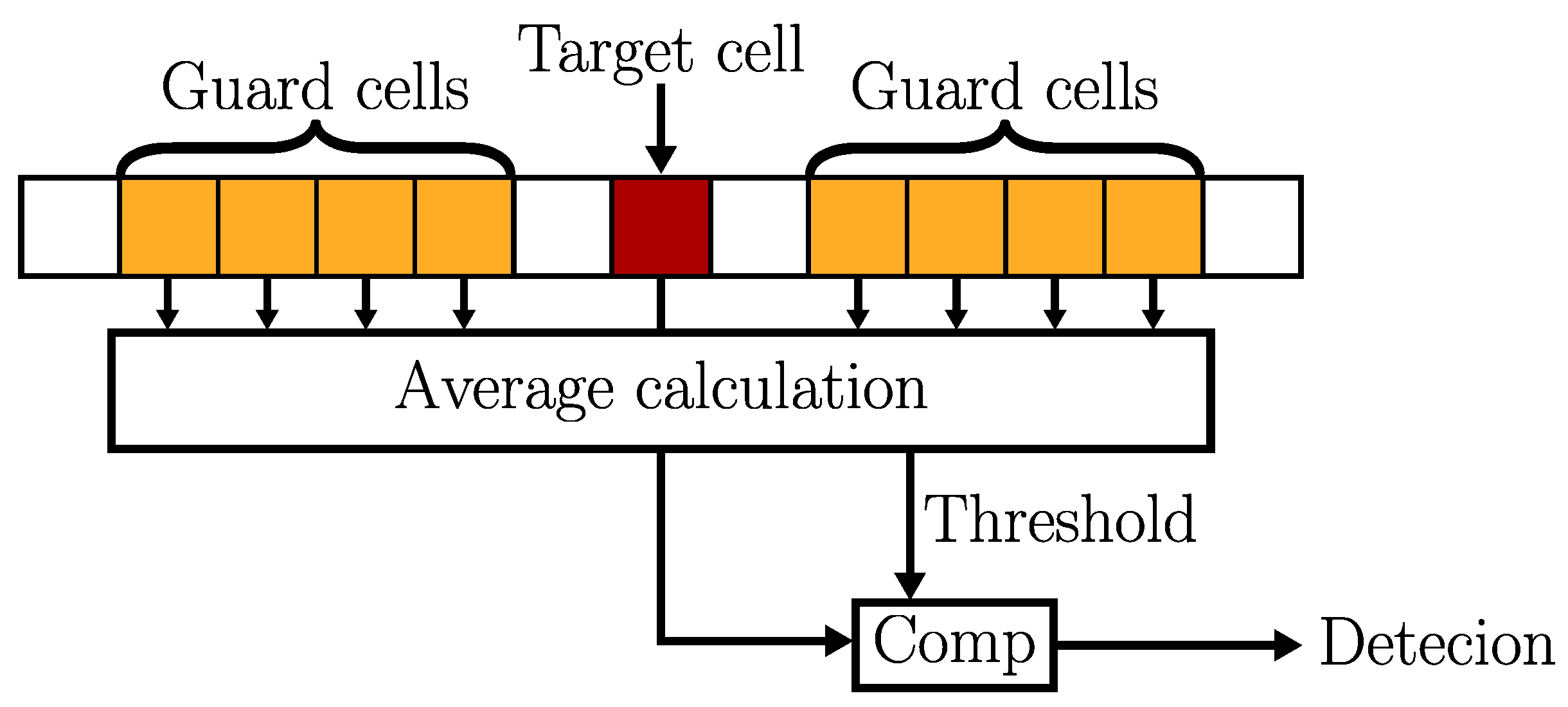
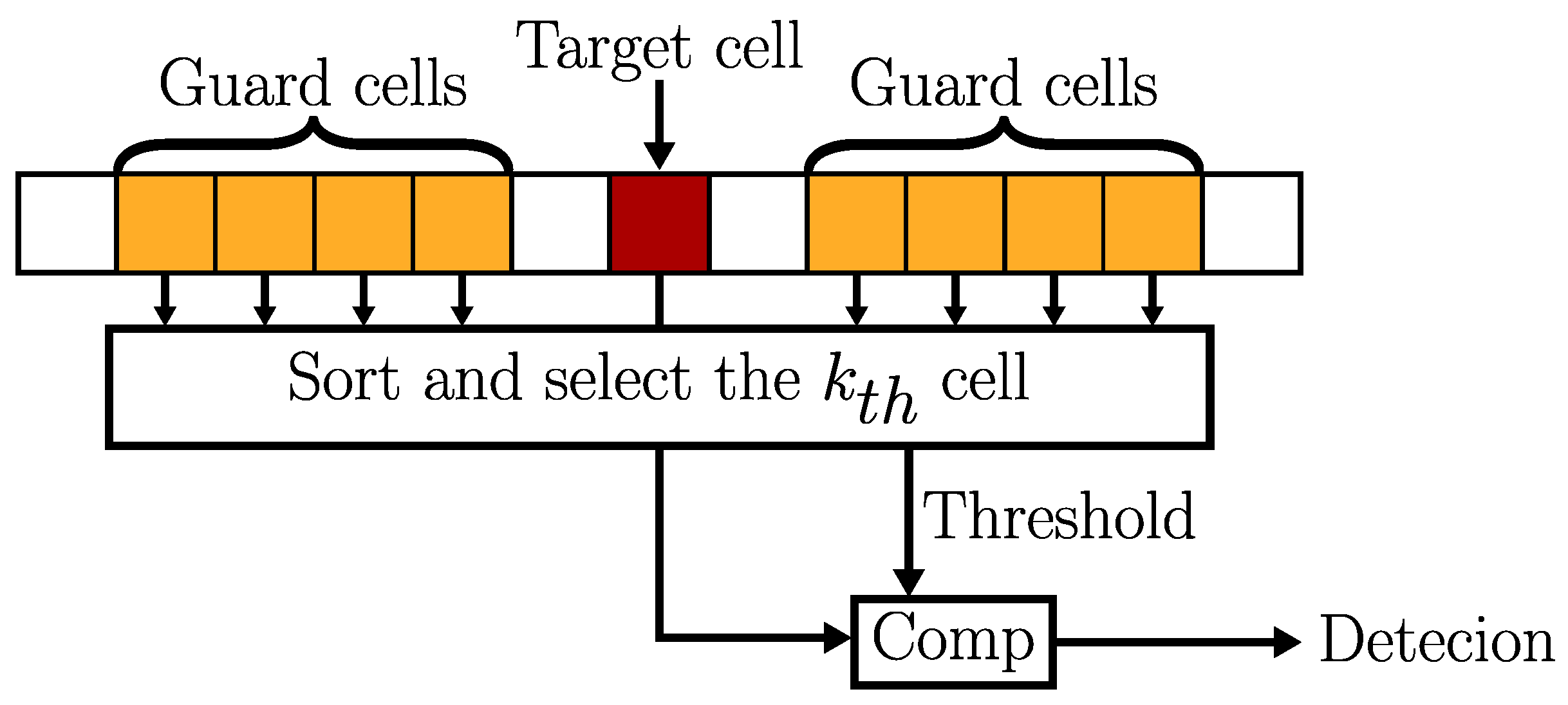
2.3. Signal Processing and Algorithms for Radars

The radar data acquisition permits to obtain the range/Doppler matrix (Figure 3) or, if the information on azimuth and elevation is available, a 4D point-cloud, but to effectively detect a target, it is necessary to test and find the points of the matrix in which the normalized power is high enough to signal the presence of a target. To do so, a threshold can be defined.

Considering the example reported in Figure 5, where a power spectrum obtained by a range/Doppler matrix is reported, two of the four highlighted bins represent actual targets: the green one and the yellow one. If the detection threshold is set to $t_1$, the yellow target will not be detected, causing a target miss. On the other hand, if the threshold is set to $t_3$, the two red spikes in the power spectrum will also be declared as detected targets (despite the fact that they are not), causing a false alarm. Indeed, threshold $t_2$ is the one that permits to detect both the green and yellow targets, ignoring the red ones.

From the presented simple example, it is evident that, to effectively detect and confirm the presence of a target, it is necessary to estimate the noise power introduced by reflections on non-relevant targets, like parked vehicles, and adapt the threshold level accordingly [21]. This permits us to reduce the probability of false alarms or to avoid ignoring relevant targets.

Many solutions to this problem have been proposed; in particular, three will be briefly discussed here: cell-averaging CFAR (CA-CFAR) [21], ordered-statistic CFAR (OS-CFAR) [39] and deep-learning-based CFAR (DL-CFAR) [40]. Figure 6 and Figure 7 report a visual comparison of the presented algorithms. As can be clearly seen, the main and only difference is in the way the threshold is estimated.

CA-CFAR estimates the detection threshold upon the range/Doppler matrix cells’ average value surrounding the target cell: if its power is higher than the average power of the surrounding cells, the target is declared [21]. This algorithm is quite simple, but in the case of two near targets, it is possible to lose the presence of one of the two.

OS-CFAR estimates the threshold by ordering the surrounding cells and selecting the value of the k-th ordered cell as the threshold. This overcomes the problem of the multiple target detection introduced by CA-CFAR algorithm, but requires us to perform the sorting of the reference cells, which is a computationally intensive task. Different sorting techniques can be used to reduce the overall computational complexity of this algorithm, as the one proposed in [41].

A different approach to CFAR problem is to use deep learning based techniques. The solution proposed by [40] is to train a neural network to recognize and remove targets from the range/Doppler map in order to estimate the noise level more precisely, without the target’s influence in the map. As reported by [40], this approach guarantees the best detection rates with respect to other CFAR algorithms, maintaining a computational cost comparable to that of the OS-CFAR.

The CFAR algorithm is used to perform the detection task. Once a target is detected, it is essential to estimate its possible trajectory. For example, to perform adaptive cruise control (ACC), it is necessary to track the velocity and position of a target vehicle and set it as a target for the host vehicle.

One of the most widespread tracking techniques relies on applying Kalman filtering [42]. This type of filter is represented by a recursive set of equations that efficiently estimates the state of a process by minimizing the mean of the squared error between the prediction and the actual measurement [43]. It is possible to directly apply this concept to tasks like Adaptive Cruise Control (ACC), where the state to be estimated is the target vehicle velocity and position [44].

The current trend in radar data processing is to adopt a deep-learning-based approach to perform object detection, recognition and tracking. Comprehensive reviews on deep learning applications to radar processing can be found in [45,46]; here, some noticeable examples are reported.

Cheng et al. [37] proposed the Radar Points Detector network (RPDnet) as a deep learning solution to the detection problem, showing promising results and a better accuracy when compared to a classical CFAR approach. As presented by Kim et al. [47], combining a Support Vector Machine (SVM) and a You Only Look Once (YOLO) model, it is possible to efficiently recognize and classify targets in radar points; in particular, they propose to identify the boundaries of the targets with the YOLO model and then use the SVM to classify them, obtaining an accuracy of 90%. Zheng et al. [48] propose Spectranet as a possible deep-learning-based approach to moving object detection and classification with an accuracy of 81.9%.

3. Lidar

Light-based measuring was initially proposed as a technique to measure the cloud-base height. This was performed by counting the time taken by a light pulse to travel to a cloud and back to the ground [49]. Middleton et al. proposed light detection and ranging (lidar) [50] as a range measuring technique. However, as with the invention of the laser [51], the lidar technique and principle became the one known nowadays: measuring the round-trip time of a laser pulse traveling to the target and back.

During recent years, lidar has become an essential component of ADAS systems; indeed, lidar systems have the possibility to guarantee automotive safety requirements [52].

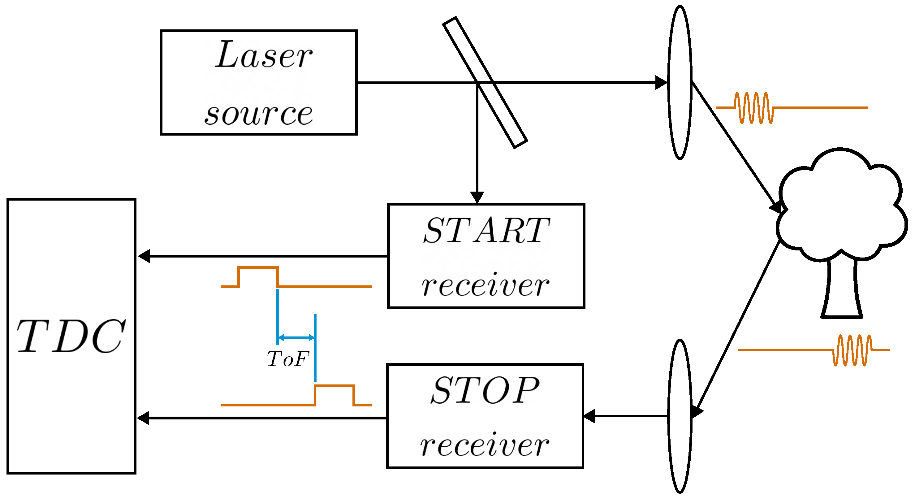
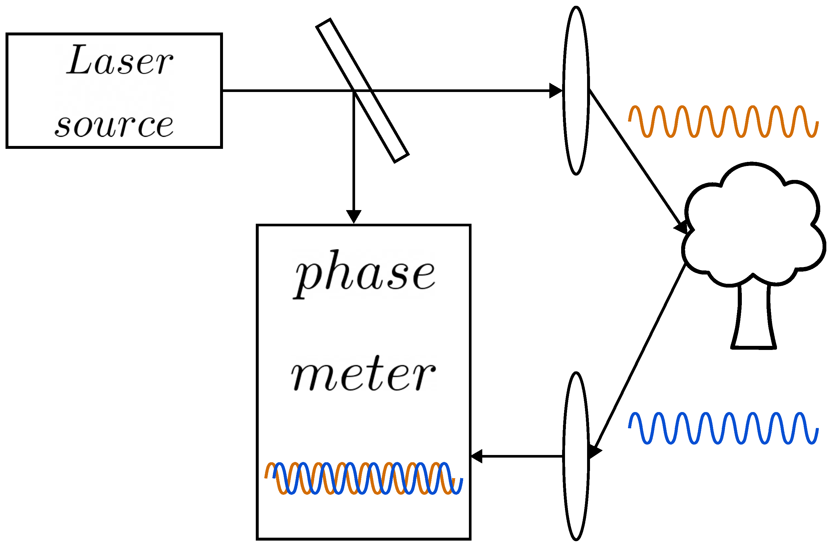
3.1. Operating Principles

Lidar’s working principle is very similar to that of the radar. Despite the idea behind them actually being the same, the main difference is that in the transmitted signal, lidar uses a laser signal instead. The simplest possible lidar is composed of a laser and a photodiode. The delay measured between the transmitted and the received light is directly proportional to the target range; the basic ruling equation of this is the same as Equation (1). It is possible to construct a 3D point-cloud representing the vehicle surroundings by measuring the time of flight (ToF), i.e., the delay $\tau$ of Equation (1), in different directions [12], defining a point-cloud whether in spherical or Cartesian coordinates depending on the type of processing and acquisition system. The 3D point-cloud can also be mixed with the GPS data to perform Simultaneous Localization and Mapping (SLAM) [53].

While the main idea remained almost unchanged, many techniques to determine the ToF and the point-cloud have been proposed, mainly working on light modulation and the way to change the laser direction to determine the 3D point-cloud.

3.2. Lidar Technology and Modulations

Currently, lidar is mainly operated with three different modulation schemes [7]:

• Pulsed ToF [54];
• Frequency Modulated Continuous Wave (FMCW) [55];
• Amplitude Modulated Continuous Wave (AMCW) [12].

Pulsed lidar relies on the direct measurement of the round-trip delay between the transmitted and the reflected signals. This is performed by means of high-resolution timers or time-to-digital converters (TDC) [56]. In particular, the transmitted pulse fires the start of a counter, while the sensing of the reflected signal stops it.

Figure 8 reports a pulsed ToF lidar scheme. First, the laser source produces a light pulse, which is detected by the start receiver that starts the count in the time to digital converter. Then, the target reflects the light pulse, which is sensed back by the stop receiver which stops the time counting. At the end, the round trip delay is measured, so Equation (1) can be applied directly to calculate the range. This technique is widely diffused, being a simple and low-cost solution [12]. Moreover, adopting the high-performance TDC presented in [56], it is possible to achieve a spatial resolution in the order of a few centimeters with a range of almost two kilometers.

In frequency-modulated continuous-wave lidars, the emitted light field is frequency modulated and an interferometric technique is applied [6] to estimate the frequency difference between the transmitted and the received signals. From the frequency difference, it is possible to estimate the distance to the target; indeed, they are proportional, as reported in Equation (5) [7]:

$$R=f_r\frac{cT}{2B},$$

(5)

where c is the speed of light, $f_r$ is the measured frequency difference, T is the duration of the modulation and B is its bandwidth.

Using a coherent detector to estimate the frequency shift introduced by the target, it is possible to obtain a system resilient to the external light sources’ interference, like the sun or lamps. Moreover, FMCW lidar introduces many other advantages, such as the possibility of estimating the target velocity by means of the Doppler shift introduced by a moving target and, operating in a continuous wave, it avoids high peak power emissions and the relative eye safety issues.

The main problem related to the use of this modulation is that it requires the use of high-performance laser and optical systems, making the whole system expensive and complex [12]. In fact, the laser has to be able to perform a wide frequency span and, at the same time, it has to maintain coherency on a wide bandwidth.

In the amplitude-modulated continuous-wave lidar, intensity modulation of a continuous light source is exploited; in particular, the round trip to the target and back introduces a phase shift proportional to the distance from the target, as reported in [7]:

$$R=\frac{c}{2}\frac{\Delta \mathsf{\Phi }}{2\pi f_M},$$

(6)

where R is the target range, c is the speed of light, $f_M$ is the amplitude modulation frequency and $\Delta \mathsf{\Phi }$ is the phase shift introduced by the target. Figure 9 reports a scheme of principle of such a system.

The modulation frequency heavily affects both the range resolution and the maximum detectable range, but it is not possible to increase the resolution without reducing the maximum range [7]. Indeed, this type of system is mainly used in near-range, high-resolution, applications.

In conclusion, the pulsed lidar seems to be the more feasible and widespread solution [12], representing a good compromise in terms of accuracy, if supported by a performing TDC, and cost, being a relatively cheap system. On the other hand, the coherent detection, both FMCW- and AMCW-based, permits it to mitigate the effects of sensing light from external sources [11].

The presented measuring methods can be used to implement different lidar imaging systems, which can be categorized into:

• Rotor-based mechanical lidar;
• Scanning solid-state lidar;
• Full solid-state lidar.

Rotor-based mechanical lidar is the most mature imaging technique used in automotive applications [12]. This can provide a ${360}^{\circ }$ horizontal field of view (FoV) by mechanically rotating the scanning system, i.e., the laser source and the receiver, while imaging along the vertical dimension is obtained by tilting the entire acquisition system or its parts, like mirrors or lenses [11].

This solution is widely used and chosen by many manufacturers, since it represents a simple but effective solution [13], even if the rotating system can be bulky and it adds some inertia to the vehicle.

An alternative to rotor-based mechanical lidar is the scanning solid-state lidar. While the former relies on rotating mechanical elements, the latter does not present any spinning mechanical parts. This permits a cheaper system with a reduced FoV. An optical phased array (OPA) [57] can be used to steer the laser beam and illuminate a specific spot at a time. On the receiver side, a similar technique [58] permits it to collect only the light arriving from the illuminated spot.

OPA-based imaging is collecting growing interest; indeed, not only it can be fully integrated on a chip, obtaining a smaller system, but the lack of inertia also permits it to increase the scanning frequency.

The full solid-state lidar is a system in which the laser source flashes and illuminates [59] all the surroundings of the vehicle. Then, an array of photodetectors collects the reflected light, and their number and density defines the spatial resolution of the imaging system. This type of system can be very expensive, due to the large number of receivers. Moreover, having to illuminate the entire FoV, the laser source requires more power than other scanning systems. Due to these limitations, solid-state lidar is applied mainly in short-range scenarios like blind-spot detection of big targets [52].

The current trend is to move in the direction of solid-state lidar [60]; this is mainly due to its lower dimension compared to the mechanically rotating lidar and the absence of inertial components.

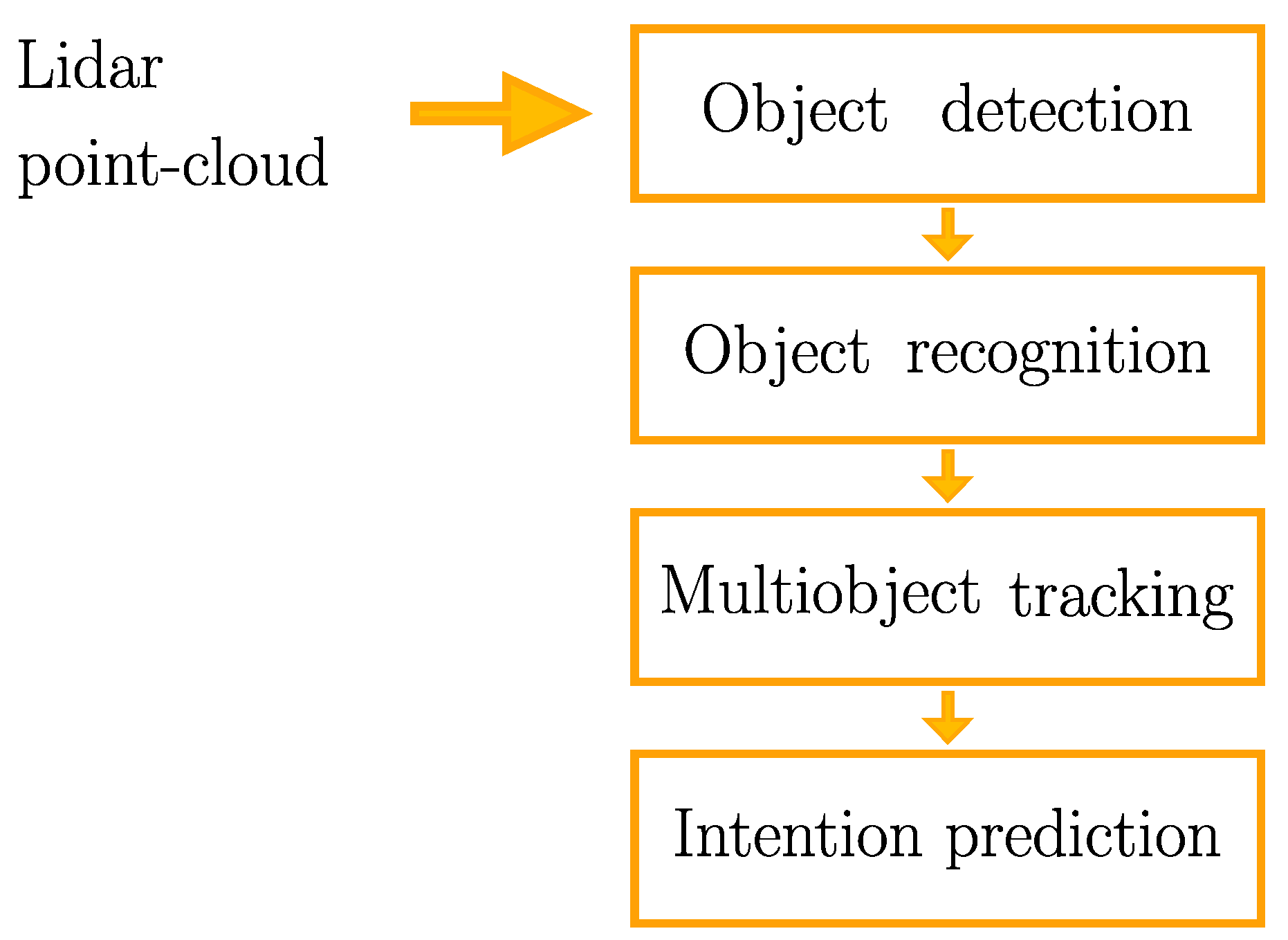
3.3. Signal Processing and Algorithms for Lidar

Lidar produces a huge amount of data to represent the 3D point-cloud, but this cannot be used as-is. Some processing has to be performed to effectively detect and recognize objects. Figure 10 reports the typical flow of a lidar-based perception system [11].

Object detection aims to extract objects in the point-cloud and to estimate their physical characteristics, such as position and shape. Lidar points can be processed in spherical coordinates. In the case of a mechanically rotating lidar, the angular information can be obtained directly by the tilt and rotation angle of the apparatus, so the range points can be clustered as they are.

Bogoslavskyi proposed an efficient clustering algorithm [61], which avoids explicitly generating the 3D point-cloud as a set of points in space, but exploits the range image generated by a scanning rotating lidar, i.e., an image in which every pixel contains the distance to the target and corresponds to a particular elevation and azimuth angle. The idea behind this clustering algorithm is to consider two neighboring points in different clusters if their depth difference is substantially larger than their displacement in the range image [61]. Some ground-filtering or weather noise removal algorithms [62] can be applied in order to remove noise from the point-cloud and perform better clustering of the points.

Following the flow in Figure 10, semantic information is added to the objects by a first feature extraction step with a subsequent classification step based on them. Many features can be used as descriptors of the detected objects [63], such as the object volume computed on its bounding box, the mean object intensity [64] or features based on the statics of the point-cloud [65,66]. Then, the extracted features are used to train and evaluate machine-learning based classifiers, like support vector machines or evidential neural networks (ENN) [67]. In particular, ENN permits it to label the objects whose features were not in the training set as unknown, reducing the labeling error rate [67].

After that, the object tracking task is performed. This can be performed by correlating the current object position with the previous one. Lee proposed a Geometric Model-Free Approach with a Particle Filter (GMFA-PF) [68] that is able to be performed during the sensing period on a single CPU and is agnostic to the shape of the tracked object; an alternative to this is the use of Kalman Filtering [11].

In conclusion, intention prediction is performed. Indeed, in an autonomous driving context, it is fundamental to predict the behavior of the detected object in order to take the correct decisions depending on the possible future behavior of the other road users. The prediction is performed mainly by the means of machine-learning methods that estimate the maneuvers of the detected object from its current state. Many driving models have been developed to predict surrounding vehicles’ behavior [69], such as theory-based, physics-based and data-driven. The behavior modeling will not be presented here. since it is beyond the interests of this review. What it is important to understand is that the lidar data can be used in such a context to provide real-time inputs to these models and support the decision-making process of autonomous driving vehicles.

The current trend is to adopt deep learning methods to extrapolate information from the lidar point-cloud [10]. Zhou et al. [70] propose VoxelNet as a deep neural network (DNN) for 3D point-cloud target detection and classification. Other examples of DNN application to lidar point-clouds are HVNet [71] and SECOND [72].

4. Sensor Fusion

In a real-life traffic urban context, it is fundamental to accurately locate and recognize other road users. To do this, the actual trend is to mix data from different sensors [73] so that the object list stored on the vehicle, i.e., the list containing all the detected road users will contain data from different sensors. For example, a vehicle velocity can be detected by radar, while its position and shape can be detected by lidar.

Sensor fusion can be performed at different levels [74]; in particular, low-level sensor data can be passed unprocessed to a fusing algorithm [75], mid-level features extracted by every sensor can be fused to define a global object list with fused features, or the high-level object lists of every sensor can be fused together in a global one.

The overall effect of sensor fusion algorithms is to obtain an object list containing objects whose features and presence has been detected by different sensors. To do so, many algorithms have been proposed in the literature [76,77].

Radar and camera data can be mixed at mid-level [78]. For example, it is possible to use the radar to detect the presence of a target in a particular area and then the visual data from the camera can be used to recognize the object in the surrounding of the detected target, avoiding the exploration of the entire image. The lidar point-cloud can be mixed with camera images [79] to add depth information to images.

5. Digital Hardware Architectures for On-Vehicle Sensing Tasks

Many sensor-related computational tasks can be accelerated in hardware. During last years, many solutions have been proposed to address different problems and algorithms, both with FPGA and ASIC implementations. Here, some examples are reported.

Subburaj et al. [80] proposed a single-chip solution for radar processing in which an FFT accelerator for the sensing task, a high performance DSP core for digital filtering and an MCU for the detection task are present. The mixed software/hardware approach guarantees a higher level of flexibility but, on the other hand, power consumption and computational efficiency are limited. The main advantage of the single-chip solution relies in the fact that, with the same system, it is possible to both drive and sample the analogue front-end, perform the detection tasks and communicate with the rest of the vehicle all with the same platform. Other noticeable implementations of single-chip radar processing systems that include hardware acceleration of computationally intensive tasks are presented in [81,82,83].

Many aspects of radar signal processing can be accelerated in hardware [84]. One of the heaviest computational tasks is the CFAR algorithm, since this needs to perform many operations on big matrices. Zhang et al. [85] report an FPGA implementation of the CA-CFAR algorithm obtaining real-time performances, while [86] reports an implementation of the ML-CFAR, i.e., a CFAR technique based on the estimation of the signal mean level. A more flexible and adaptive approach to the CFAR problem is presented by [87]. A highly parametrizable and configurable implementation is reported in [88], which features 7 different CFAR algorithms and guarantees real time performances. Other noticeable hardware implementations of the CFAR algorithm are discussed in [89,90,91].

The literature provides other examples of hardware accelerators for radar data processing.

Damnjanović et al. [92] present a CHISEL model to generate 2D-FFT accelerators, both for basic range-Doppler processing and specialized for range-angle processing; they also present a custom memory controller to deal with radar data. Saponara [84] proposes a set of hardware macrocells to perform detection starting from the base-band signal. In particular, range, Doppler and azimuth processing is performed with a set of hardware FFT, while a hardware implementation of CA-CFAR is adopted to perform peak detection.

A speed up in the overall processing can be introduced by performing the interference mitigation task on the range-Doppler matrix in hardware; for example, Hirschmugl et al. [93] propose a quantized Convolutional Neural Network (CNN) implementation to perform this task directly in the frequency domain before the object detection task, and the hardware implementation is $7.7$ times faster than the presented firmware implementation.

Another hardware-compliant task is the early detection and recognition of obstacles; indeed, this is a priority task, since it is necessary to rapidly stop the vehicle if an obstacle is present and different alarm signals can be produced depending on the type of target. A system that can perform this task in real time is presented in [94]. In [95], it is possible to find an early detection hardware system that guarantees a valid detection in 41.72 $\mathsf{\mu }$s, giving optimal performances to the emergency breaking system. A deep learning approach that is based on quantized YOLO CNNs can be found in [96].

The problem of direction of arrival estimation is addressed in [97]; the authors present a hardware architecture to perform maximum-likelihood direction of arrival estimation that is 7 times faster than the proposed software version.

Table 2. Examples of full radar detection system.

	Implemented Tasks	Main Features	Implementation	${\mathit{f}}_{\mathit{op}}$ [MHz]	Processing Time
[80]	Waveform generation, FFT computation, data compression, target detection (OS-CFAR)	Single-chip solution with RF front-end, DSP, MCU and HW accelerators	45 nm CMOS	360
[81]	Analog-to-digital converter, RISC-V general purpose core, FIR filter, polyphase filter, FFT	Single-chip solution for radar processing based on a RISC-V system	16 nm FinFET	410
[82]	FIR filtering, FFT, OS-CFAR	Complete radar processing flow	(Virtex7 485T FPGA)
[83]	Complete object detection	Hardware acceleration of 2D-FFT, detection and angle estimation	Integrate SoC available by Texas Instrument (AM273x SoC)	200
[84]	Full target detection processing: 3D-FFT, CA-CFAR	Range, Doppler and azimuth processing, integrated with peak detection	Around 36,000 (XA7A100T FPGA)	200	$51.2$ ms

,

Table 3. Examples of radar hardware accelerators for CFAR.

	Implemented Tasks	Main Features	Implementation	${\mathit{f}}_{\mathit{op}}$ [MHz]	Processing Time
[85]	2D CA-CFAR	Special purpose hardware, computation and hardware complexity reduction avoiding repeated calculations	2816 LUTs (xc7a100tcsg324-1 FPGA)	$114.19$
[86]	2D ML-CFAR	Many configurable parameters, such as reference window size and protection window size	8000 LUTs (xc6vlx240t FPGA)	220
[87]	custom-CFAR	Proposal of a new CFAR algorithm, efficient sorting architecture	8260 LUTs (Altera Stratix II)	$118.39$	0.6 $\mathsf{\mu }$s
[89]	B-ACOSD CFAR	Efficient HW/SW partition of the CFAR algorithm on an Altera-based system	4723 LUTs (Altera Stratix IV)	250	0.45 $\mathsf{\mu }$s
[90]	ACOSD-CFAR	Efficient HW/SW partition of the CFAR algorithm on an Xilinx-based system	10,441 LUTs (Zedboard Zynq 7000)	148	0.24 $\mathsf{\mu }$s
[88]	Peak detector generator	Seven types of different CFAR algorithms available	From 630 to 7453 LUTs depending on the selected parameters (Xilinx Spartan-7)	100

and

Table 4. Examples of radar hardware accelerators.

	Implemented Tasks	Main Features	Implementation	${\mathit{f}}_{\mathit{op}}$ [MHz]	Processing Time
[92]	Range-Doppler processing, specialized range-angle processing, SDRAM controller for radar data processing	Parametrized hardware generators for 2D-FFT, range-Doppler and range-angle	From around 1000 to 60,000 LUTs, depending on the selected parameters		real time processing
[93]	Interference mitigation	Quantized CNN model working with range-Doppler matrix	$30\%$ of available LUTs (Xilinx Zynq 7000)	100	32.8–44.4 ms
[97]	Direction of arrival	CORDIC based maximum-likelihood direction of arrival estimation, many configuration parameters available	From 900 to 14,500 LUTs depending on the selected parameters (XC7VX485T Xilinx Virtex-7)	200
[94]	Early obstacle detection and recognition	Early warning and collision avoidance system	10,688 LUTs (Xilinx Virtex 6)		15.86 ms
[95]	Early obstacle detection	Configurable early detection system	27,808 LUTs (Nexys Video Artix 7)	200	41.72 $\mathsf{\mu }$s
[96]	Obstacle detection and tracking	Deep-learning-based detection and tracking	Around 38,000 LUTs (Xilinx Zynq 7000)	230	10.9 ms per frame

report a brief overview of the presented hardware accelerators, mainly focusing on the implemented tasks and main reported features. Operating frequency ($f_{op}$) and implementation information are also reported.

A commercial lidar (for example the Velodyne VLS-128) can produce a point-cloud at a rate of 9.6 Mpoints/s [98]. This can be quite a high data rate to be handled in real-time, so a hardware-accelerated data compression strategy, such as the one presented in [98], can be adopted to deal with real-time performances.

In the context of lidar sensing, many tasks can be accelerated in hardware; they are mainly related to the point-cloud data processing, which is performed by adopting machine learning techniques. Therefore, the acceleration of neural networks is required. Some implementation of this type of accelerators specialized for lidar processing are present in the literature [99,100]. Another computationally heavy task is the weather denoising of the point-cloud; this can also be accelerated in hardware, as proposed in [101]. Real-time lidar localization can also be accelerated; in particular, Bernardi et al. [102] present a hardware accelerator for particle filter on an FPGA platform to perform this task in real time.

A completely different approach to accelerate on-vehicle sensor processing is the use of GPU [103]; indeed, many lidar point-cloud related processing algorithms can be parallelized and efficiently executed on GPUs.

Table 5. Examples of lidar hardware accelerators.

	Implemented Tasks	Main Features	Implementation
[100]	Point-cloud segmentation and classification	Implements the PointNet network on an FPGA platform	19,530 LUTs (Xilinx Zynq UltraScale+)
[99]	Convolutions, rectified linear unit (ReLU), padding and max pooling	General purpose CNN accelerator	10,832 LUTs (Zybo Z7:Zynq 7000)
[102]	Real-time localization	Hardware acceleration of ray marching for particle filter	186,430 LUTs (Ultra96 XCU102)

summarizes the implemented tasks and main features of the presented accelerators for lidar-related computational tasks; the number of LUTs used in the reported FPGA implementation is also reported.

6. Comparison and Conclusions

In conclusion, the idea behind radar and lidar is very similar, and many common aspects have been highlighted. However, some differences have to be considered.

Table 6. Table with differences between radar and lidar.

	Radar	Lidar
Transmitted signal	RF signal	laser signal
Signal source	mm-wave antenna	laser
Signal receiver	mm-wave antenna	photodiode
Output	4D array (Range Doppler DoA Elevation)	3D point-cloud
Range	long	short
Range resolution	low	high
Angular resolution	low	high
Radial velocity resolution	high	low

presents a qualitative comparison between radar an lidar. First of all, the transmitted signal is different; indeed, radar uses RF signal, while lidar uses laser. Lidar produces a temporal consistent 3D point-cloud, while it is almost impossible to guarantee time consistency in radar detection array. Moreover, the DSP/data processing flow is quite different [13]. From the performance point of view, lidar is more feasible when short-range and high-resolution capabilities are required, for example in a city-like scenario, while radar is more feasible when it is necessary to detect far fast-moving targets, like in a highway scenario [74].

One of the main challenges for radar development is the low angular resolution. In fact, to achieve the sub-degree resolution of lidar, a large radar aperture, or a high number of antennas, is required making the actual on-vehicle integration unfeasible. On the other hand, lidar is a very expensive system, and its operational range remains quite limited due to eye-safety restrictions [13]. Both sensing systems present many open challenges, and the research is still active both from academic and industrial point of view.

This review’s aim was to summarize the main aspects and the state-of-the-art of these two important technologies and to highlight their differences and open points relative to these two sensing systems.

References

1. Grimes, D.; Jones, T. Automotive radar: A brief review. Proc. IEEE 1974, 62, 804–822. [Google Scholar] [CrossRef]
2. Fölster, F.; Rohling, H. Signal processing structure for automotive radar. Frequenz 2006, 60, 20–24. [Google Scholar] [CrossRef]
3. Hasch, J.; Topak, E.; Schnabel, R.; Zwick, T.; Weigel, R.; Waldschmidt, C. Millimeter-Wave Technology for Automotive Radar Sensors in the 77 GHz Frequency Band. IEEE Trans. Microw. Theory Tech. 2012, 60, 845–860. [Google Scholar] [CrossRef]
4. Hakobyan, G.; Yang, B. High-Performance Automotive Radar: A Review of Signal Processing Algorithms and Modulation Schemes. IEEE Signal Process. Mag. 2019, 36, 32–44. [Google Scholar] [CrossRef]
5. Patole, S.M.; Torlak, M.; Wang, D.; Ali, M. Automotive radars: A review of signal processing techniques. IEEE Signal Process. Mag. 2017, 34, 22–35. [Google Scholar] [CrossRef]
6. Behroozpour, B.; Sandborn, P.A.M.; Wu, M.C.; Boser, B.E. Lidar System Architectures and Circuits. IEEE Commun. Mag. 2017, 55, 135–142. [Google Scholar] [CrossRef]
7. Royo, S.; Ballesta-Garcia, M. An Overview of Lidar Imaging Systems for Autonomous Vehicles. Appl. Sci. 2019, 9, 4093. [Google Scholar] [CrossRef]
8. Gharineiat, Z.; Kurdi, F.T.; Campbell, G. Review of Automatic Processing of Topography and Surface Feature Identification LiDAR Data Using Machine Learning Techniques. Remote Sens. 2022, 14, 4685. [Google Scholar] [CrossRef]
9. Mirzaei, K.; Arashpour, M.; Asadi, E.; Masoumi, H.; Bai, Y.; Behnood, A. 3D point cloud data processing with machine learning for construction and infrastructure applications: A comprehensive review. Adv. Eng. Inform. 2022, 51, 101501. [Google Scholar] [CrossRef]
10. Alaba, S.Y.; Ball, J.E. A Survey on Deep-Learning-Based LiDAR 3D Object Detection for Autonomous Driving. Sensors 2022, 22, 9577. [Google Scholar] [CrossRef]
11. Li, Y.; Ibanez-Guzman, J. Lidar for Autonomous Driving: The Principles, Challenges, and Trends for Automotive Lidar and Perception Systems. IEEE Signal Process. Mag. 2020, 37, 50–61. [Google Scholar] [CrossRef]
12. Roriz, R.; Cabral, J.; Gomes, T. Automotive LiDAR Technology: A Survey. IEEE Trans. Intell. Transp. Syst. 2022, 23, 6282–6297. [Google Scholar] [CrossRef]
13. Bilik, I. Comparative Analysis of Radar and Lidar Technologies for Automotive Applications. IEEE Intell. Transp. Syst. Mag. 2023, 15, 244–269. [Google Scholar] [CrossRef]
14. James, R. A history of radar. IEE Rev. 1989, 35, 343. [Google Scholar] [CrossRef]
15. Fan, R.; Wang, L.; Bocus, M.J.; Pitas, I. Computer Stereo Vision for Autonomous Driving: Theory and Algorithms. In Studies in Computational Intelligence; Springer International Publishing: Cham, Switzerland, 2023; pp. 41–70. [Google Scholar] [CrossRef]
16. Skolnik, M.I. Introduction to Radar Systems; McGraw-Hill Education: Noida, India, 2018. [Google Scholar]
17. Alizadeh, M.; Shaker, G.; Almeida, J.C.M.D.; Morita, P.P.; Safavi-Naeini, S. Remote Monitoring of Human Vital Signs Using mm-Wave FMCW Radar. IEEE Access 2019, 7, 54958–54968. [Google Scholar] [CrossRef]
18. Kronauge, M.; Rohling, H. New chirp sequence radar waveform. IEEE Trans. Aerosp. Electron. Syst. 2014, 50, 2870–2877. [Google Scholar] [CrossRef]
19. Gill, T. The Doppler Effect: An Introduction to the Theory of the Effect; Scientific Monographs on Physics; Logos Press: Moscow, ID, USA, 1965. [Google Scholar]
20. Winkler, V. Range Doppler detection for automotive FMCW radars. In Proceedings of the 2007 European Radar Conference, Munich, Germany, 10–12 October 2007. [Google Scholar] [CrossRef]
21. Rohling, H. Radar CFAR Thresholding in Clutter and Multiple Target Situations. IEEE Trans. Aerosp. Electron. Syst. 1983, AES-19, 608–621. [Google Scholar] [CrossRef]
22. Bourdoux, A.; Ahmad, U.; Guermandi, D.; Brebels, S.; Dewilde, A.; Thillo, W.V. PMCW waveform and MIMO technique for a 79 GHz CMOS automotive radar. In Proceedings of the 2016 IEEE Radar Conference (RadarConf), Philadelphia, PA, USA, 2–6 May 2016. [Google Scholar] [CrossRef]
23. Sur, S.N.; Sharma, P.; Saikia, H.; Banerjee, S.; Singh, A.K. OFDM Based RADAR-Communication System Development. Procedia Comput. Sci. 2020, 171, 2252–2260. [Google Scholar] [CrossRef]
24. Beise, H.P.; Stifter, T.; Schroder, U. Virtual interference study for FMCW and PMCW radar. In Proceedings of the 2018 11th German Microwave Conference (GeMiC), Freiburg, Germany, 12–14 March 2018. [Google Scholar] [CrossRef]
25. Levanon, N.; Mozeson, E. Matched Filter. In Radar Signals; John Wiley & Sons, Ltd.: Hoboken, NJ, USA, 2004; Chapter 2; pp. 20–33. [Google Scholar] [CrossRef]
26. Langevin, P. Some sequences with good autocorrelation properties. In Contemporary Mathematics; American Mathematical Society: Providence, RI, USA, 1994. [Google Scholar] [CrossRef]
27. Jungnickel, D.; Pott, A. Perfect and almost perfect sequences. Discret. Appl. Math. 1999, 95, 331–359. [Google Scholar] [CrossRef]
28. Knill, C.; Embacher, F.; Schweizer, B.; Stephany, S.; Waldschmidt, C. Coded OFDM Waveforms for MIMO Radars. IEEE Trans. Veh. Technol. 2021, 70, 8769–8780. [Google Scholar] [CrossRef]
29. Braun, M.; Sturm, C.; Jondral, F.K. On the single-target accuracy of OFDM radar algorithms. In Proceedings of the 2011 IEEE 22nd International Symposium on Personal, Indoor and Mobile Radio Communications, Toronto, ON, Canada, 11–14 September 2011. [Google Scholar] [CrossRef]
30. Sturm, C.; Wiesbeck, W. Waveform Design and Signal Processing Aspects for Fusion of Wireless Communications and Radar Sensing. Proc. IEEE 2011, 99, 1236–1259. [Google Scholar] [CrossRef]
31. Fink, J.; Jondral, F.K. Comparison of OFDM radar and chirp sequence radar. In Proceedings of the 2015 16th International Radar Symposium (IRS), Dresden, Germany, 24–26 June 2015. [Google Scholar] [CrossRef]
32. Vasanelli, C.; Roos, F.; Durr, A.; Schlichenmaier, J.; Hugler, P.; Meinecke, B.; Steiner, M.; Waldschmidt, C. Calibration and Direction-of-Arrival Estimation of Millimeter-Wave Radars: A Practical Introduction. IEEE Antennas Propag. Mag. 2020, 62, 34–45. [Google Scholar] [CrossRef]
33. Duly, A.J.; Love, D.J.; Krogmeier, J.V. Time-Division Beamforming for MIMO Radar Waveform Design. IEEE Trans. Aerosp. Electron. Syst. 2013, 49, 1210–1223. [Google Scholar] [CrossRef]
34. Feger, R.; Pfeffer, C.; Stelzer, A. A Frequency-Division MIMO FMCW Radar System Based on Delta–Sigma Modulated Transmitters. IEEE Trans. Microw. Theory Tech. 2014, 62, 3572–3581. [Google Scholar] [CrossRef]
35. Sun, Y.; Bauduin, M.; Bourdoux, A. Enhancing Unambiguous Velocity in Doppler-Division Multiplexing MIMO Radar. In Proceedings of the 2021 18th European Radar Conference (EuRAD), London, UK, 5–7 April 2022. [Google Scholar] [CrossRef]
36. Sun, S.; Petropulu, A.P.; Poor, H.V. MIMO Radar for Advanced Driver-Assistance Systems and Autonomous Driving: Advantages and Challenges. IEEE Signal Process. Mag. 2020, 37, 98–117. [Google Scholar] [CrossRef]
37. Cheng, Y.; Su, J.; Chen, H.; Liu, Y. A New Automotive Radar 4D Point Clouds Detector by Using Deep Learning. In Proceedings of the ICASSP 2021–2021 IEEE International Conference on Acoustics, Speech and Signal Processing (ICASSP), Toronto, ON, Canada, 6–11 June 2021. [Google Scholar] [CrossRef]
38. Han, Z.; Wang, J.; Xu, Z.; Yang, S.; He, L.; Xu, S.; Wang, J. 4D Millimeter-Wave Radar in Autonomous Driving: A Survey. arXiv 2023, arXiv:2306.04242. [Google Scholar] [CrossRef]
39. Magaz, B.; Belouchrani, A.; Hamadouche, M. Automatic threshold selection in OS-CFAR radar detection using information theoretic criteria. Prog. Electromagn. Res. B 2011, 30, 157–175. [Google Scholar] [CrossRef]
40. Lin, C.H.; Lin, Y.C.; Bai, Y.; Chung, W.H.; Lee, T.S.; Huttunen, H. DL-CFAR: A Novel CFAR Target Detection Method Based on Deep Learning. In Proceedings of the 2019 IEEE 90th Vehicular Technology Conference (VTC2019-Fall), Honolulu, HI, USA, 22–25 September 2019. [Google Scholar] [CrossRef]
41. Hyun, E.; Lee, J.H. A New OS-CFAR Detector Design. In Proceedings of the 2011 First ACIS/JNU International Conference on Computers, Networks, Systems and Industrial Engineering, Jeju, Republic of Korea, 23–25 May 2011. [Google Scholar] [CrossRef]
42. Macaveiu, A.; Campeanu, A. Automotive radar target tracking by Kalman filtering. In Proceedings of the 2013 11th International Conference on Telecommunications in Modern Satellite, Cable and Broadcasting Services (TELSIKS), Nis, Serbia, 16–19 October 2013. [Google Scholar] [CrossRef]
43. Chen, B.; Dang, L.; Zheng, N.; Principe, J.C. Kalman Filtering. In Kalman Filtering Under Information Theoretic Criteria; Springer International Publishing: Cham, Switzerland, 2023; pp. 11–51. [Google Scholar] [CrossRef]
44. Wu, C.; Lin, Y.; Eskandarian, A. Cooperative Adaptive Cruise Control with Adaptive Kalman Filter Subject to Temporary Communication Loss. IEEE Access 2019, 7, 93558–93568. [Google Scholar] [CrossRef]
45. Lang, P.; Fu, X.; Martorella, M.; Dong, J.; Qin, R.; Meng, X.; Xie, M. A Comprehensive Survey of Machine Learning Applied to Radar Signal Processing. arXiv 2020, arXiv:abs/2009.13702. [Google Scholar]
46. Geng, Z.; Yan, H.; Zhang, J.; Zhu, D. Deep-Learning for Radar: A Survey. IEEE Access 2021, 9, 141800–141818. [Google Scholar] [CrossRef]
47. Kim, W.; Cho, H.; Kim, J.; Kim, B.; Lee, S. Target Classification Using Combined YOLO-SVM in High-Resolution Automotive FMCW Radar. In Proceedings of the 2020 IEEE Radar Conference (RadarConf20), Florence, Italy, 21–25 September 2020. [Google Scholar] [CrossRef]
48. Zheng, R.; Sun, S.; Scharff, D.; Wu, T. Spectranet: A High Resolution Imaging Radar Deep Neural Network for Autonomous Vehicles. In Proceedings of the 2022 IEEE 12th Sensor Array and Multichannel Signal Processing Workshop (SAM), Trondheim, Norway, 20–23 June 2022. [Google Scholar] [CrossRef]
49. Hulburt, E.O. Observations of a Searchlight Beam to an Altitude of 28 Kilometers. J. Opt. Soc. Am. 1937, 27, 377–382. [Google Scholar] [CrossRef]
50. Middleton, W.E.K.; Spilhaus, A.F. Meteorological Instruments. Q. J. R. Meteorol. Soc. 1954, 80, 484. [Google Scholar] [CrossRef]
51. Maiman, T.H. Stimulated Optical Radiation in Ruby. Nature 1960, 187, 493–494. [Google Scholar] [CrossRef]
52. Warren, M.E. Automotive LIDAR Technology. In Proceedings of the 2019 Symposium on VLSI Circuits, Kyoto, Japan, 9–14 June 2019. [Google Scholar] [CrossRef]
53. Chen, C.; Xiong, G.; Zhang, Z.; Gong, J.; Qi, J.; Wang, C. 3D LiDAR-GPS/IMU Calibration Based on Hand-Eye Calibration Model for Unmanned Vehicle. In Proceedings of the 2020 3rd International Conference on Unmanned Systems (ICUS), Harbin, China, 27–28 November 2020. [Google Scholar] [CrossRef]
54. Liu, J.; Sun, Q.; Fan, Z.; Jia, Y. TOF Lidar Development in Autonomous Vehicle. In Proceedings of the 2018 IEEE 3rd Optoelectronics Global Conference (OGC), Shenzhen, China, 4–7 September 2018. [Google Scholar] [CrossRef]
55. Dieckmann, A.; Amann, M.C. Frequency-modulated continuous-wave (FMCW) lidar with tunable twin-guide laser diode. In Automated 3D and 2D Vision; Kamerman, G.W., Keicher, W.E., Eds.; SPIE’s 1994 International Symposium on Optics, Imaging, and Instrumentation: San Diego, CA, USA, 1994. [Google Scholar] [CrossRef]
56. Hejazi, A.; Oh, S.; Rehman, M.R.U.; Rad, R.E.; Kim, S.; Lee, J.; Pu, Y.; Hwang, K.C.; Yang, Y.; Lee, K.Y. A Low-Power Multichannel Time-to-Digital Converter Using All-Digital Nested Delay-Locked Loops with 50-ps Resolution and High Throughput for LiDAR Sensors. IEEE Trans. Instrum. Meas. 2020, 69, 9262–9271. [Google Scholar] [CrossRef]
57. Kim, T.; Ngai, T.; Timalsina, Y.; Watts, M.R.; Stojanovic, V.; Bhargava, P.; Poulton, C.V.; Notaros, J.; Yaacobi, A.; Timurdogan, E.; et al. A Single-Chip Optical Phased Array in a Wafer-Scale Silicon Photonics/CMOS 3D-Integration Platform. IEEE J. Solid State Circuits 2019, 54, 3061–3074. [Google Scholar] [CrossRef]
58. Fatemi, R.; Abiri, B.; Khachaturian, A.; Hajimiri, A. High sensitivity active flat optics optical phased array receiver with a two-dimensional aperture. Opt. Express 2018, 26, 29983. [Google Scholar] [CrossRef]
59. Lemmetti, J.; Sorri, N.; Kallioniemi, I.; Melanen, P.; Uusimaa, P. Long-range all-solid-state flash LiDAR sensor for autonomous driving. In High-Power Diode Laser Technology XIX; Zediker, M.S., Ed.; SPIE Digital Library: Bellingham, WA, USA, 2021. [Google Scholar] [CrossRef]
60. Li, N.; Ho, C.P.; Xue, J.; Lim, L.W.; Chen, G.; Fu, Y.H.; Lee, L.Y.T. A Progress Review on Solid-State LiDAR and Nanophotonics-Based LiDAR Sensors. Laser Photonics Rev. 2022, 16, 2100511. [Google Scholar] [CrossRef]
61. Bogoslavskyi, I.; Stachniss, C. Fast range image-based segmentation of sparse 3D laser scans for online operation. In Proceedings of the 2016 IEEE/RSJ International Conference on Intelligent Robots and Systems (IROS), Daejeon, Republic of Korea, 9–14 October 2016. [Google Scholar] [CrossRef]
62. Le, M.H.; Cheng, C.H.; Liu, D.G. An Efficient Adaptive Noise Removal Filter on Range Images for LiDAR Point Clouds. Electronics 2023, 12, 2150. [Google Scholar] [CrossRef]
63. Chen, T.; Dai, B.; Liu, D.; Song, J. Performance of global descriptors for velodyne-based urban object recognition. In Proceedings of the 2014 IEEE Intelligent Vehicles Symposium Proceedings, Dearborn, MI, USA, 8–11 June 2014. [Google Scholar] [CrossRef]
64. Himmelsbach, M.; Mueller, A.D.I.; Luettel, T.; Wunsche, H.J. LIDAR-based 3 D Object Perception. In Proceedings of the 1st International Workshop on Cognition for Technical Systems, Munich, Germany, 6–8 October 2008. [Google Scholar]
65. Anguelov, D.; Taskar, B.; Chatalbashev, V.; Koller, D.; Gupta, D.; Heitz, G.; Ng, A. Discriminative Learning of Markov Random Fields for Segmentation of 3D Scan Data. In Proceedings of the 2005 IEEE Computer Society Conference on Computer Vision and Pattern Recognition (CVPR’05), San Diego, CA, USA, 20–25 June 2005. [Google Scholar] [CrossRef]
66. Lalonde, J.F.; Vandapel, N.; Huber, D.F.; Hebert, M. Natural terrain classification using three-dimensional ladar data for ground robot mobility. J. Field Robot. 2006, 23, 839–861. [Google Scholar] [CrossRef]
67. Capellier, E.; Davoine, F.; Cherfaoui, V.; Li, Y. Evidential deep learning for arbitrary LIDAR object classification in the context of autonomous driving. In Proceedings of the 2019 IEEE Intelligent Vehicles Symposium (IV), Paris, France, 9–12 June 2019. [Google Scholar] [CrossRef]
68. Lee, H.; Lee, H.; Shin, D.; Yi, K. Moving Objects Tracking Based on Geometric Model-Free Approach with Particle Filter Using Automotive LiDAR. IEEE Trans. Intell. Transp. Syst. 2022, 23, 17863–17872. [Google Scholar] [CrossRef]
69. Negash, N.M.; Yang, J. Driver Behavior Modeling Toward Autonomous Vehicles: Comprehensive Review. IEEE Access 2023, 11, 22788–22821. [Google Scholar] [CrossRef]
70. Zhou, Y.; Tuzel, O. VoxelNet: End-to-End Learning for Point Cloud Based 3D Object Detection. In Proceedings of the 2018 IEEE/CVF Conference on Computer Vision and Pattern Recognition, Salt Lake City, UT, USA, 18–22 June 2018. [Google Scholar] [CrossRef]
71. Ye, M.; Xu, S.; Cao, T. HVNet: Hybrid Voxel Network for LiDAR Based 3D Object Detection. In Proceedings of the 2020 IEEE/CVF Conference on Computer Vision and Pattern Recognition (CVPR), Seattle, WA, USA, 14–19 June 2020. [Google Scholar] [CrossRef]
72. Yan, Y.; Mao, Y.; Li, B. SECOND: Sparsely Embedded Convolutional Detection. Sensors 2018, 18, 3337. [Google Scholar] [CrossRef] [PubMed]
73. Senel, N.; Kefferpütz, K.; Doycheva, K.; Elger, G. Multi-Sensor Data Fusion for Real-Time Multi-Object Tracking. Processes 2023, 11, 501. [Google Scholar] [CrossRef]
74. Steinbaeck, J.; Steger, C.; Holweg, G.; Druml, N. Next generation radar sensors in automotive sensor fusion systems. In Proceedings of the 2017 Sensor Data Fusion: Trends, Solutions, Applications (SDF), Bonn, Germany, 10–12 October 2017. [Google Scholar] [CrossRef]
75. Walchshäusl, L.; Lindl, R.; Vogel, K.; Tatschke, T. Detection of Road Users in Fused Sensor Data Streams for Collision Mitigation. In Advanced Microsystems for Automotive Applications 2006; Springer: Berlin/Heidelberg, Germany, 2006; pp. 53–65. [Google Scholar] [CrossRef]
76. Chen, H.; Kirubarajan, T. Performance limits of track-to-track fusion versus centralized estimation: Theory and application. IEEE Trans. Aerosp. Electron. Syst. 2003, 39, 386–400. [Google Scholar] [CrossRef]
77. Wang, X.; Xu, L.; Sun, H.; Xin, J.; Zheng, N. On-Road Vehicle Detection and Tracking Using MMW Radar and Monovision Fusion. IEEE Trans. Intell. Transp. Syst. 2016, 17, 2075–2084. [Google Scholar] [CrossRef]
78. Zhou, Y.; Dong, Y.; Hou, F.; Wu, J. Review on Millimeter-Wave Radar and Camera Fusion Technology. Sustainability 2022, 14, 5114. [Google Scholar] [CrossRef]
79. Bai, X.; Hu, Z.; Zhu, X.; Huang, Q.; Chen, Y.; Fu, H.; Tai, C.L. TransFusion: Robust LiDAR-Camera Fusion for 3D Object Detection with Transformers. In Proceedings of the 2022 IEEE/CVF Conference on Computer Vision and Pattern Recognition (CVPR), New Orleans, LA, USA, 19–24 June 2022. [Google Scholar] [CrossRef]
80. Subburaj, K.; Narayanan, N.; Mani, A.; Ramasubramanian, K.; Ramalingam, S.; Nayyar, J.; Dandu, K.; Bhatia, K.; Arora, M.; Jayanthi, S.; et al. Single-Chip 77GHz FMCW Automotive Radar with Integrated Front-End and Digital Processing. In Proceedings of the 2022 23rd International Radar Symposium (IRS), Gdansk, Poland, 12–14 September 2022. [Google Scholar] [CrossRef]
81. Bailey, S.; Rigge, P.; Han, J.; Lin, R.; Chang, E.Y.; Mao, H.; Wang, Z.; Markley, C.; Izraelevitz, A.M.; Wang, A.; et al. A Mixed-Signal RISC-V Signal Analysis SoC Generator with a 16-nm FinFET Instance. IEEE J. Solid State Circuits 2019, 54, 2786–2801. [Google Scholar] [CrossRef]
82. Meinl, F.; Stolz, M.; Kunert, M.; Blume, H. An experimental high performance radar system for highly automated driving. In Proceedings of the 2017 IEEE MTT-S International Conference on Microwaves for Intelligent Mobility (ICMIM), Nagoya, Japan, 19–21 March 2017. [Google Scholar] [CrossRef]
83. Nagalikar, S.; Mody, M.; Baranwal, A.; Kumar, V.; Shankar, P.; Farooqui, M.A.; Shah, M.; Sangani, N.; Rakesh, Y.; Karkisaval, A.; et al. Single Chip Radar Processing for Object Detection. In Proceedings of the 2023 IEEE International Conference on Consumer Electronics (ICCE), Las Vegas, NV, USA, 6–8 January 2023. [Google Scholar] [CrossRef]
84. Saponara, S. Hardware accelerator IP cores for real time Radar and camera-based ADAS. J. Real Time Image Process. 2016, 16, 1493–1510. [Google Scholar] [CrossRef]
85. Zhang, M.; Li, X. An Efficient Real-Time Two-Dimensional CA-CFAR Hardware Engine. In Proceedings of the 2019 IEEE International Conference on Electron Devices and Solid-State Circuits (EDSSC), Xi’an, China, 12–14 June 2019. [Google Scholar] [CrossRef]
86. Tao, X.; Zhang, D.; Wang, M.; Ma, Y.; Song, Y. Design and Implementation of A High-speed Configurable 2D ML-CFAR Detector. In Proceedings of the 2021 IEEE 14th International Conference on ASIC (ASICON), Kunming, China, 26–29 October 2021. [Google Scholar] [CrossRef]
87. Sim, Y.; Heo, J.; Jung, Y.; Lee, S.; Jung, Y. FPGA Implementation of Efficient CFAR Algorithm for Radar Systems. Sensors 2023, 23, 954. [Google Scholar] [CrossRef]
88. Petrovic, M.L.; Milovanovic, V.M. A Design Generator of Parametrizable and Runtime Configurable Constant False Alarm Rate Processors. In Proceedings of the 2021 28th IEEE International Conference on Electronics, Circuits, and Systems (ICECS), Dubai, United Arab Emirates, 28 November–1 December 2021. [Google Scholar] [CrossRef]
89. Djemal, R.; Belwafi, K.; Kaaniche, W.; Alshebeili, S.A. An FPGA-based implementation of HW/SW architecture for CFAR radar target detector. In Proceedings of the ICM 2011 Proceeding, Hammamet, Tunisia, 19–22 December 2011. [Google Scholar] [CrossRef]
90. Msadaa, S.; Lahbib, Y.; Mami, A. A SoPC FPGA Implementing of an Enhanced Parallel CFAR Architecture. In Proceedings of the 2022 IEEE 9th International Conference on Sciences of Electronics, Technologies of Information and Telecommunications (SETIT), Hammamet, Tunisia, 28–30 May 2022. [Google Scholar] [CrossRef]
91. Bharti, V.K.; Patel, V. Realization of real time adaptive CFAR processor for homing application in marine environment. In Proceedings of the 2018 Conference on Signal Processing And Communication Engineering Systems (SPACES), Vijayawada, India, 4–5 January 2018. [Google Scholar] [CrossRef]
92. Damnjanović, V.D.; Petrović, M.L.; Milovanović, V.M. On Hardware Implementations of Two-Dimensional Fast Fourier Transform for Radar Signal Processing. In Proceedings of the IEEE EUROCON 2023–20th International Conference on Smart Technologies, Torino, Italy, 6–8 July 2023. [Google Scholar] [CrossRef]
93. Hirschmugl, M.; Rock, J.; Meissner, P.; Pernkopf, F. Fast and resource-efficient CNNs for Radar Interference Mitigation on Embedded Hardware. In Proceedings of the 2022 19th European Radar Conference (EuRAD), Milan, Italy, 28–30 September 2022. [Google Scholar] [CrossRef]
94. Liu, H.; Niar, S.; El-Hillali, Y.; Rivenq, A. Embedded architecture with hardware accelerator for target recognition in driver assistance system. ACM SIGARCH Comput. Archit. News 2011, 39, 56–59. [Google Scholar] [CrossRef]
95. Petrović, N.; Petrović, M.; Milovanović, V. Radar Signal Processing Architecture for Early Detection of Automotive Obstacles. Electronics 2023, 12, 1826. [Google Scholar] [CrossRef]
96. Zhai, J.; Li, B.; Lv, S.; Zhou, Q. FPGA-Based Vehicle Detection and Tracking Accelerator. Sensors 2023, 23, 2208. [Google Scholar] [CrossRef] [PubMed]
97. Meinl, F.; Kunert, M.; Blume, H. Hardware acceleration of Maximum-Likelihood angle estimation for automotive MIMO radars. In Proceedings of the 2016 Conference on Design and Architectures for Signal and Image Processing (DASIP), Rennes, France, 12–14 October 2016. [Google Scholar] [CrossRef]
98. Cunha, L.; Roriz, R.; Pinto, S.; Gomes, T. Hardware-Accelerated Data Decoding and Reconstruction for Automotive LiDAR Sensors. IEEE Trans. Veh. Technol. 2023, 72, 4267–4276. [Google Scholar] [CrossRef]
99. Silva, J.; Pereira, P.; Machado, R.; Névoa, R.; Melo-Pinto, P.; Fernandes, D. Customizable FPGA-Based Hardware Accelerator for Standard Convolution Processes Empowered with Quantization Applied to LiDAR Data. Sensors 2022, 22, 2184. [Google Scholar] [CrossRef]
100. Bai, L.; Lyu, Y.; Xu, X.; Huang, X. PointNet on FPGA for Real-Time LiDAR Point Cloud Processing. In Proceedings of the 2020 IEEE International Symposium on Circuits and Systems (ISCAS), Seville, Spain, 12–14 October 2020. [Google Scholar] [CrossRef]
101. Roriz, R.; Campos, A.; Pinto, S.; Gomes, T. DIOR: A Hardware-Assisted Weather Denoising Solution for LiDAR Point Clouds. IEEE Sens. J. 2022, 22, 1621–1628. [Google Scholar] [CrossRef]
102. Bernardi, A.; Brilli, G.; Capotondi, A.; Marongiu, A.; Burgio, P. An FPGA Overlay for Efficient Real-Time Localization in 1/10th Scale Autonomous Vehicles. In Proceedings of the 2022 Design, Automation & Test in Europe Conference & Exhibition (DATE), Antwerp, Belgium, 14–23 March 2022. [Google Scholar] [CrossRef]
103. Venugopal, V.; Kannan, S. Accelerating real-time LiDAR data processing using GPUs. In Proceedings of the 2013 IEEE 56th International Midwest Symposium on Circuits and Systems (MWSCAS), Columbus, OH, USA, 4–7 August 2013. [Google Scholar] [CrossRef]
Figure 1. Radar operating principle.
Chips 02 00015 g001
Figure 2. Basic scheme of an FMCW radar.
Chips 02 00015 g002
Figure 3. Range Doppler matrix with a target at distance d t and velocity v t .
Chips 02 00015 g003
Figure 4. PMCW radar block diagram.
Chips 02 00015 g004
Figure 5. Illustration of the power spectrum along a column of the range/Doppler matrix.
Chips 02 00015 g005
Figure 6. Cell-averaging CFAR.
Chips 02 00015 g006
Figure 7. Ordered statistics CFAR.
Chips 02 00015 g007
Figure 8. ToF lidar scheme.
Chips 02 00015 g008
Figure 9. Scheme of the principle of an AMCW lidar system.
Chips 02 00015 g009
Figure 10. Typical lidar perception flow.
Chips 02 00015 g010