
Low-Altitude, Overcooled Scree Slope: Insights into Temperature Distribution Using High-Resolution Thermal Imagery in the Romanian Carpathians

 ,
,  and
and
Abstract
:1. Introduction
2. Methodology and Materials
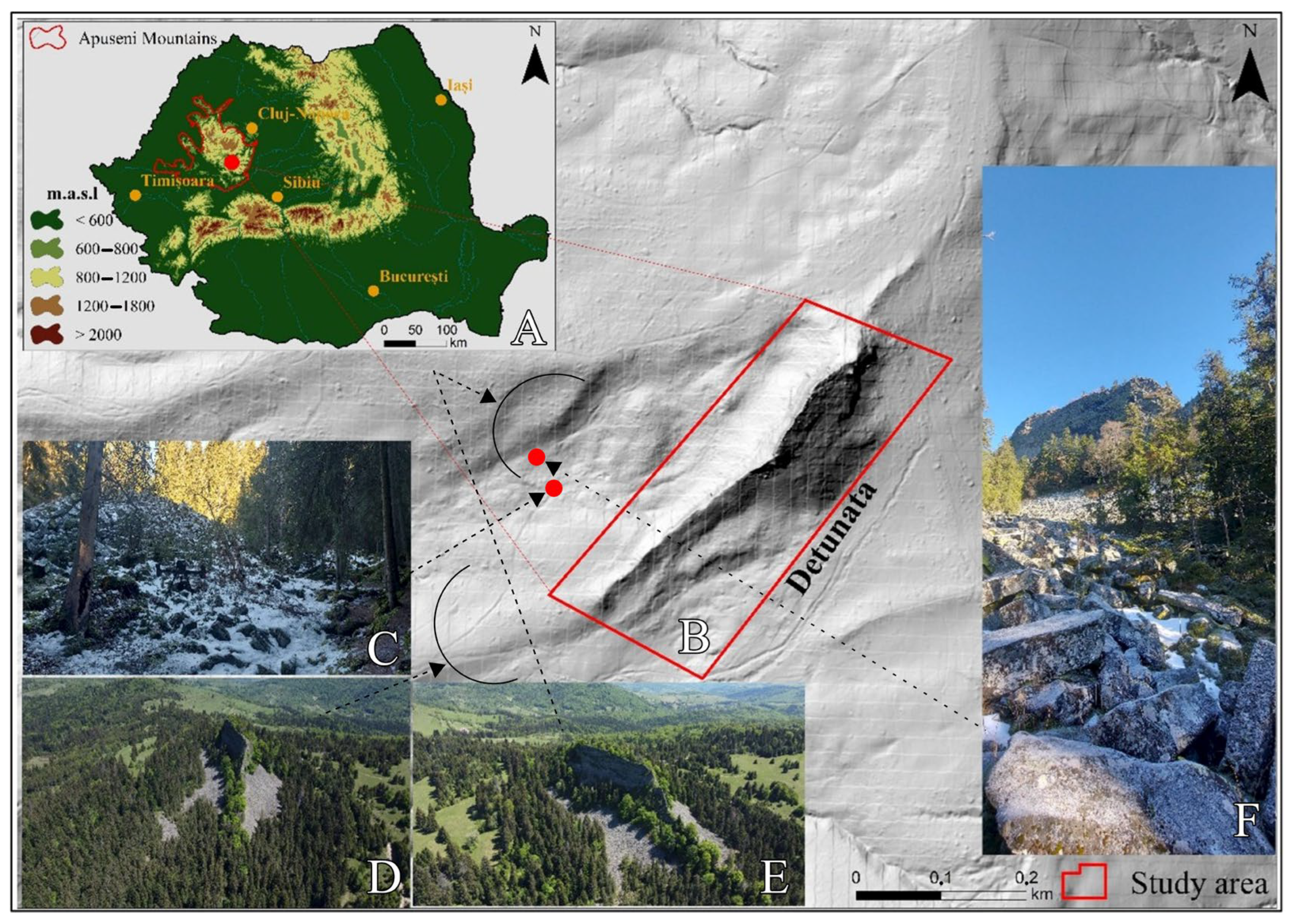
2.1. Study Area
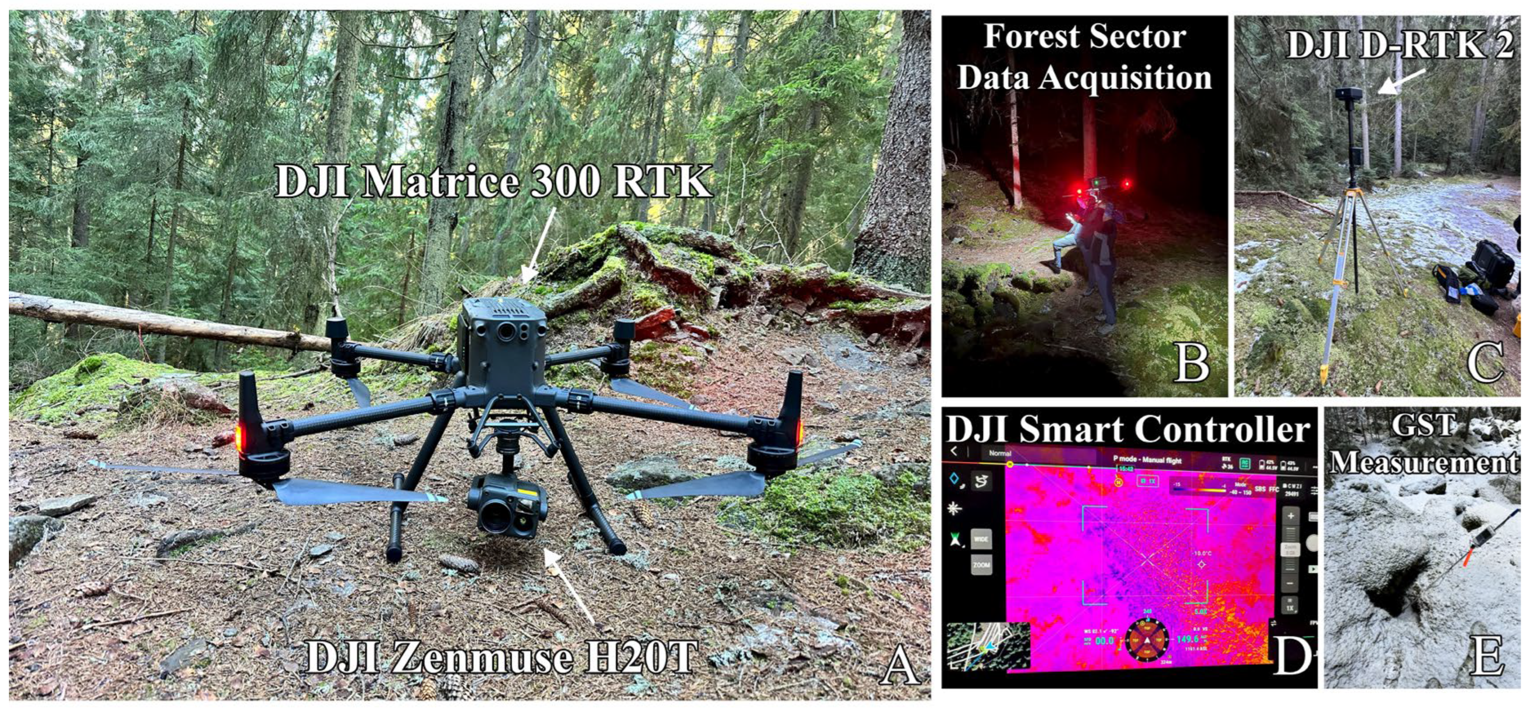
2.2. Methodology
3. Results
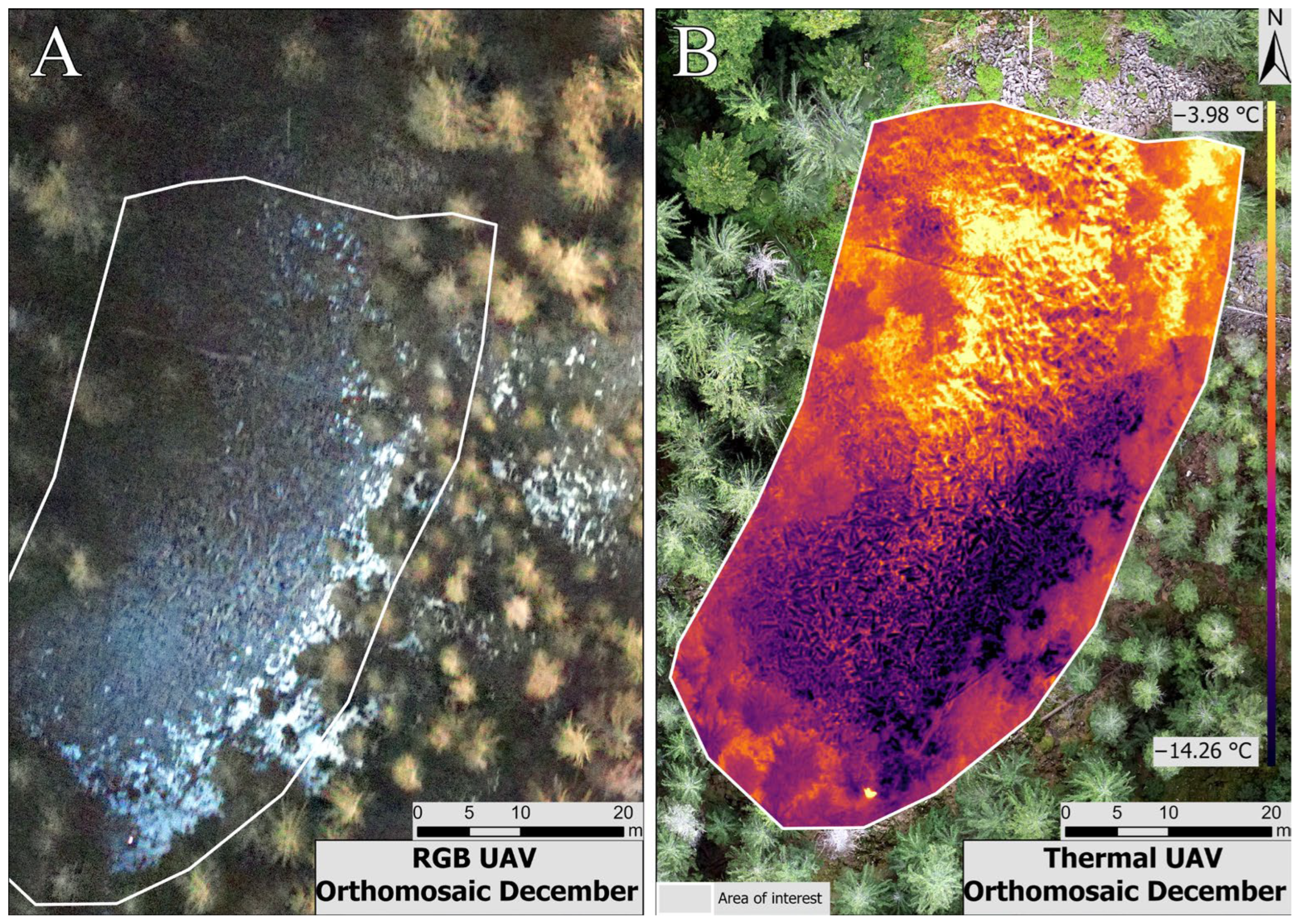
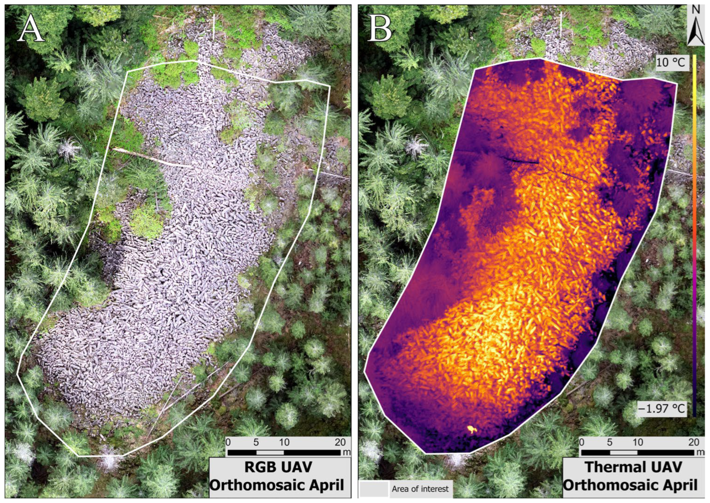
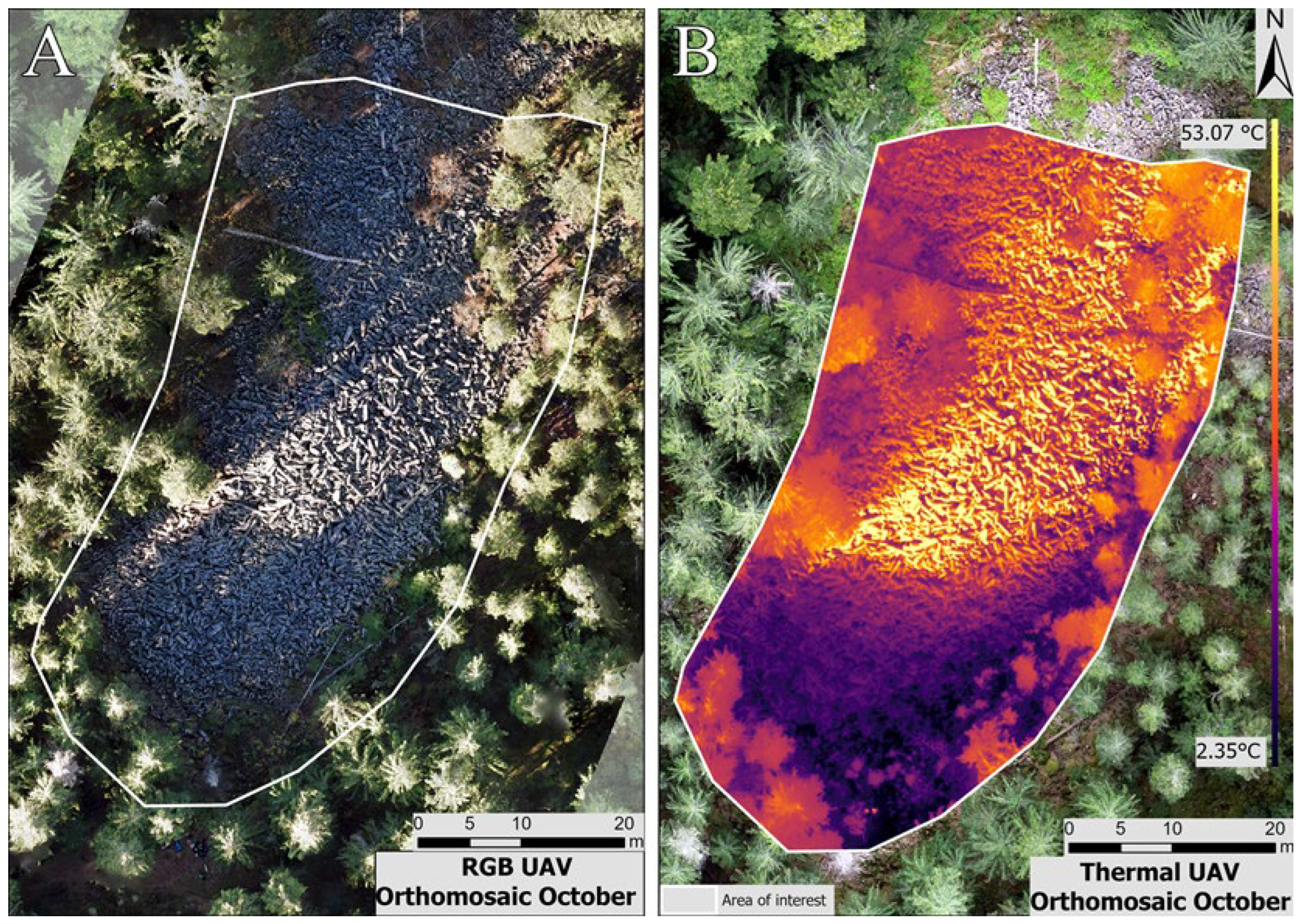
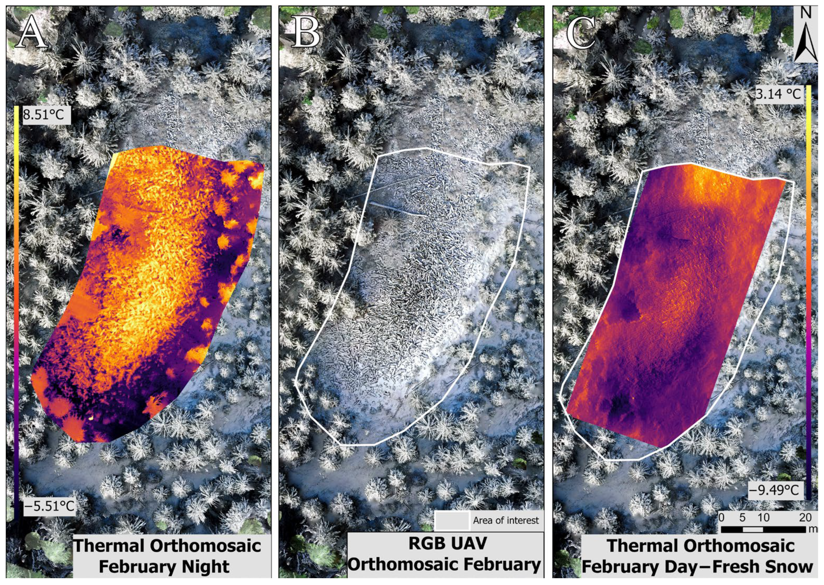
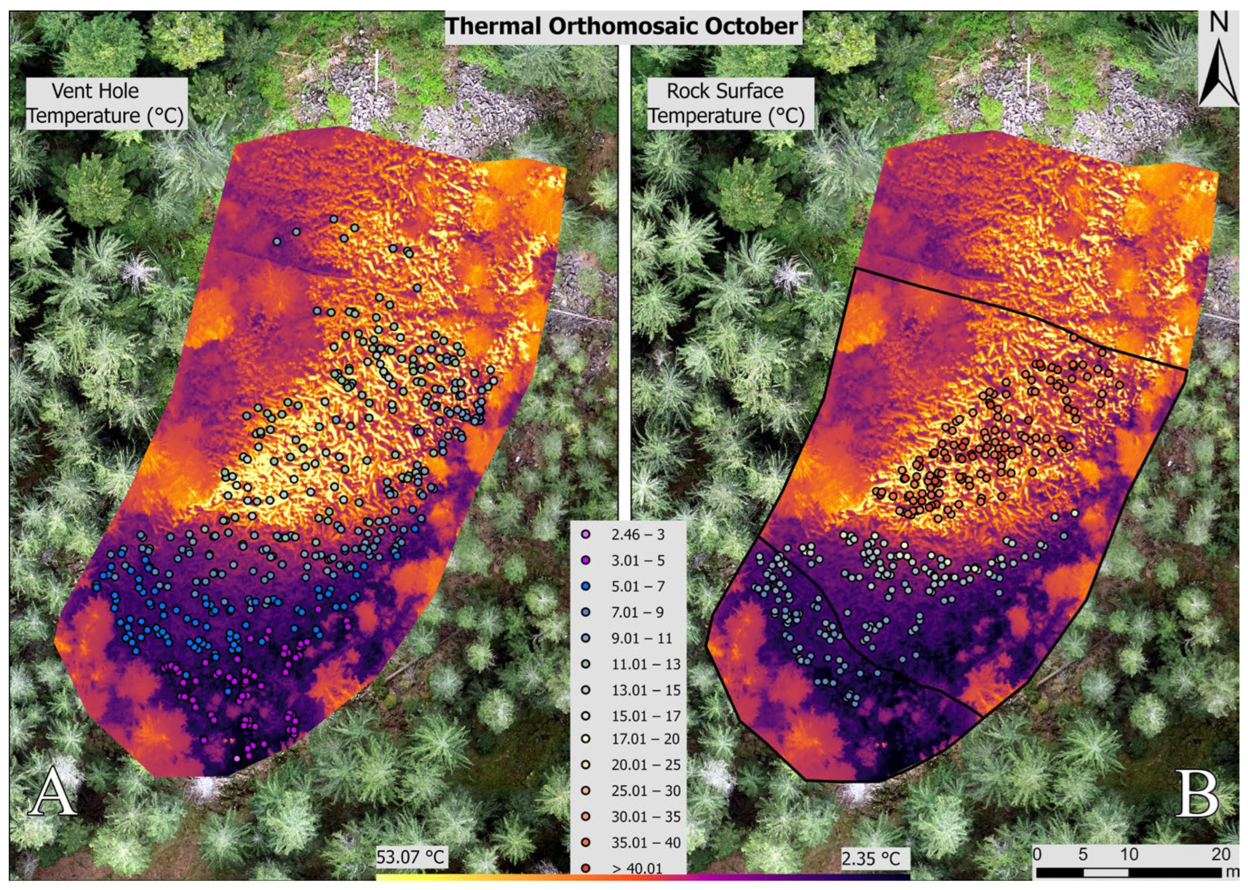
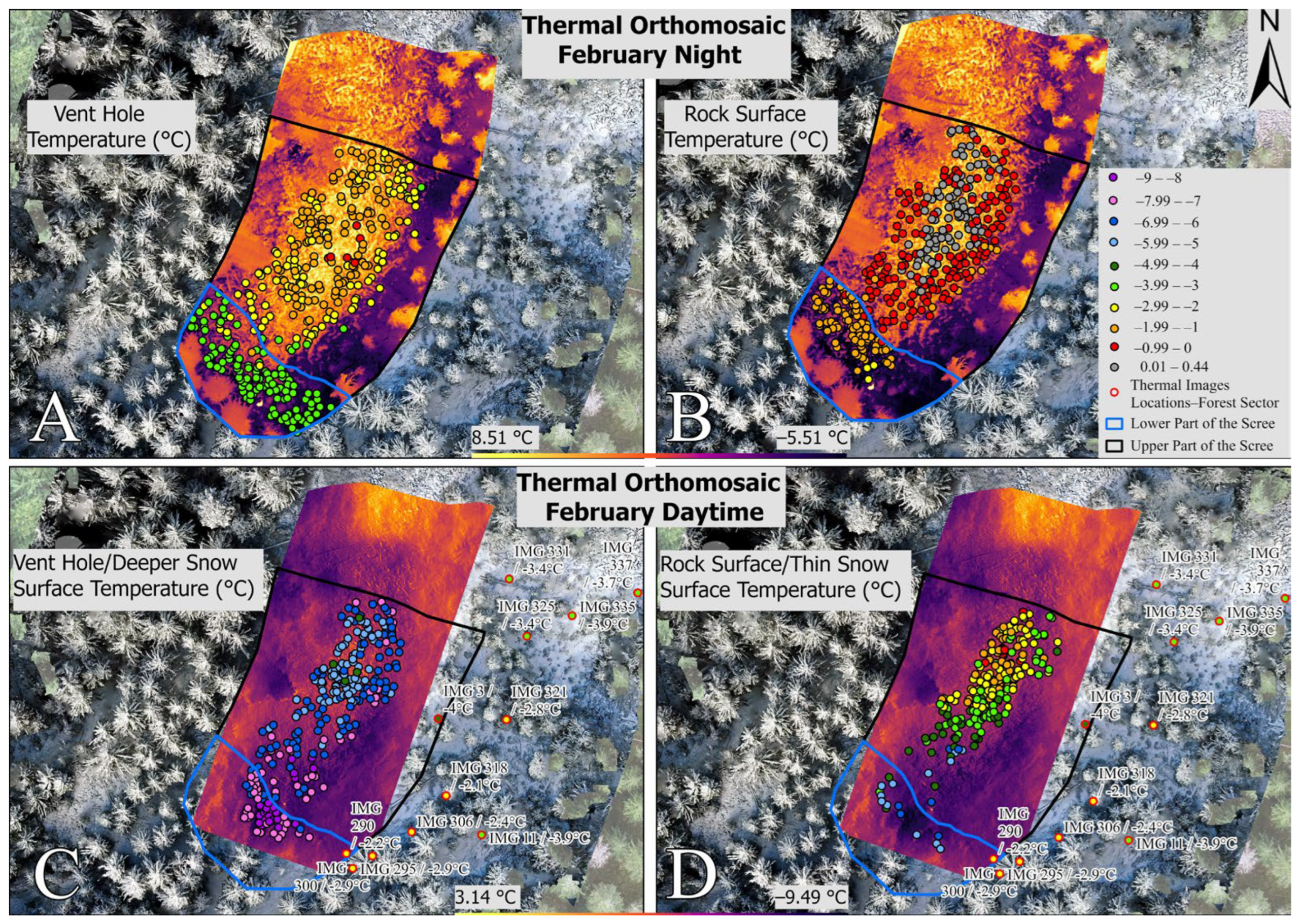
3.1. UAV-Derived Thermal and RGB Maps
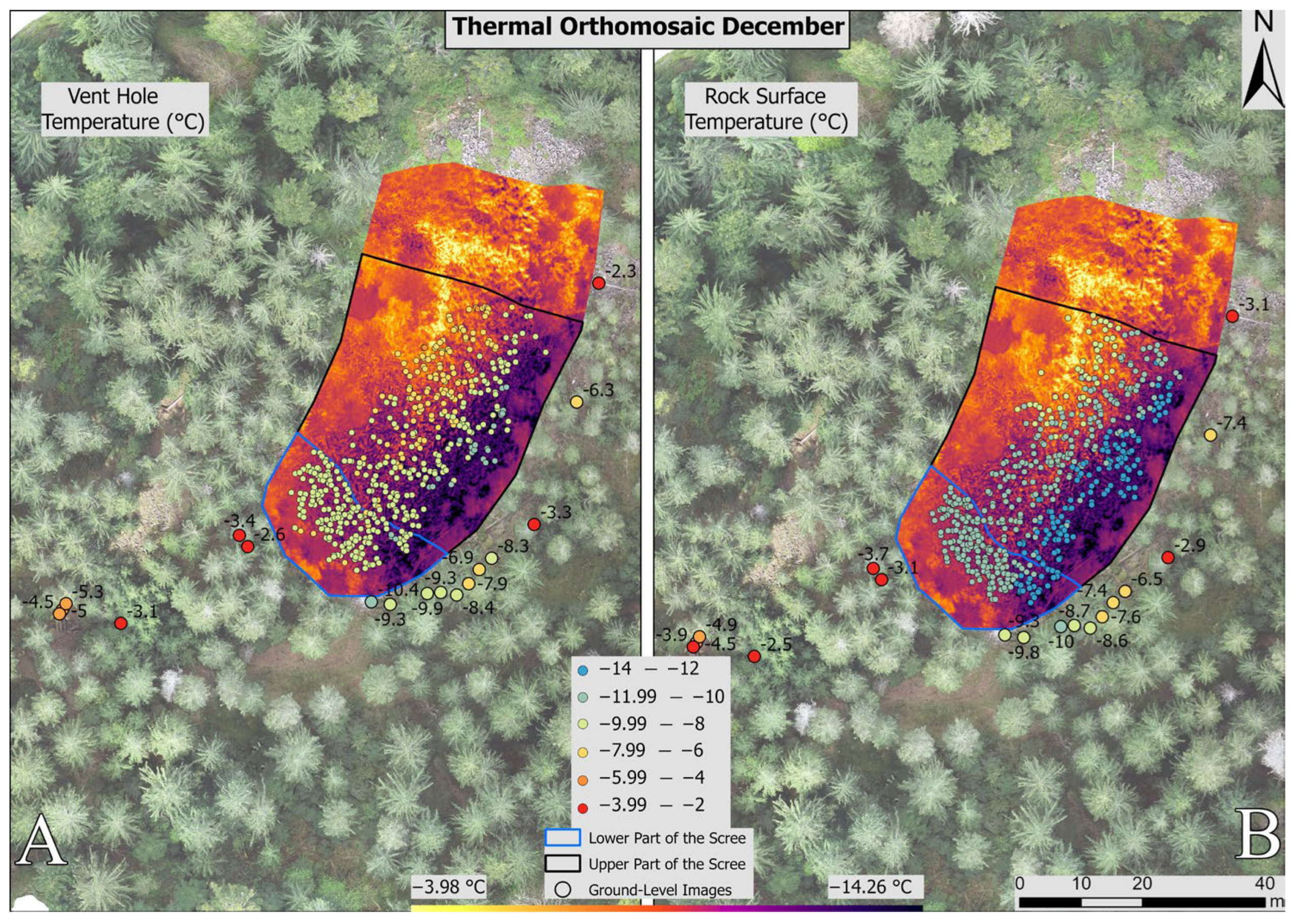
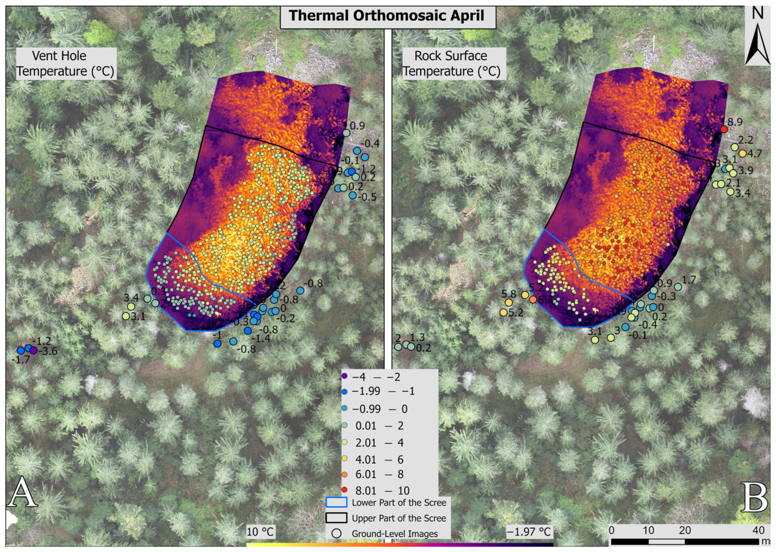
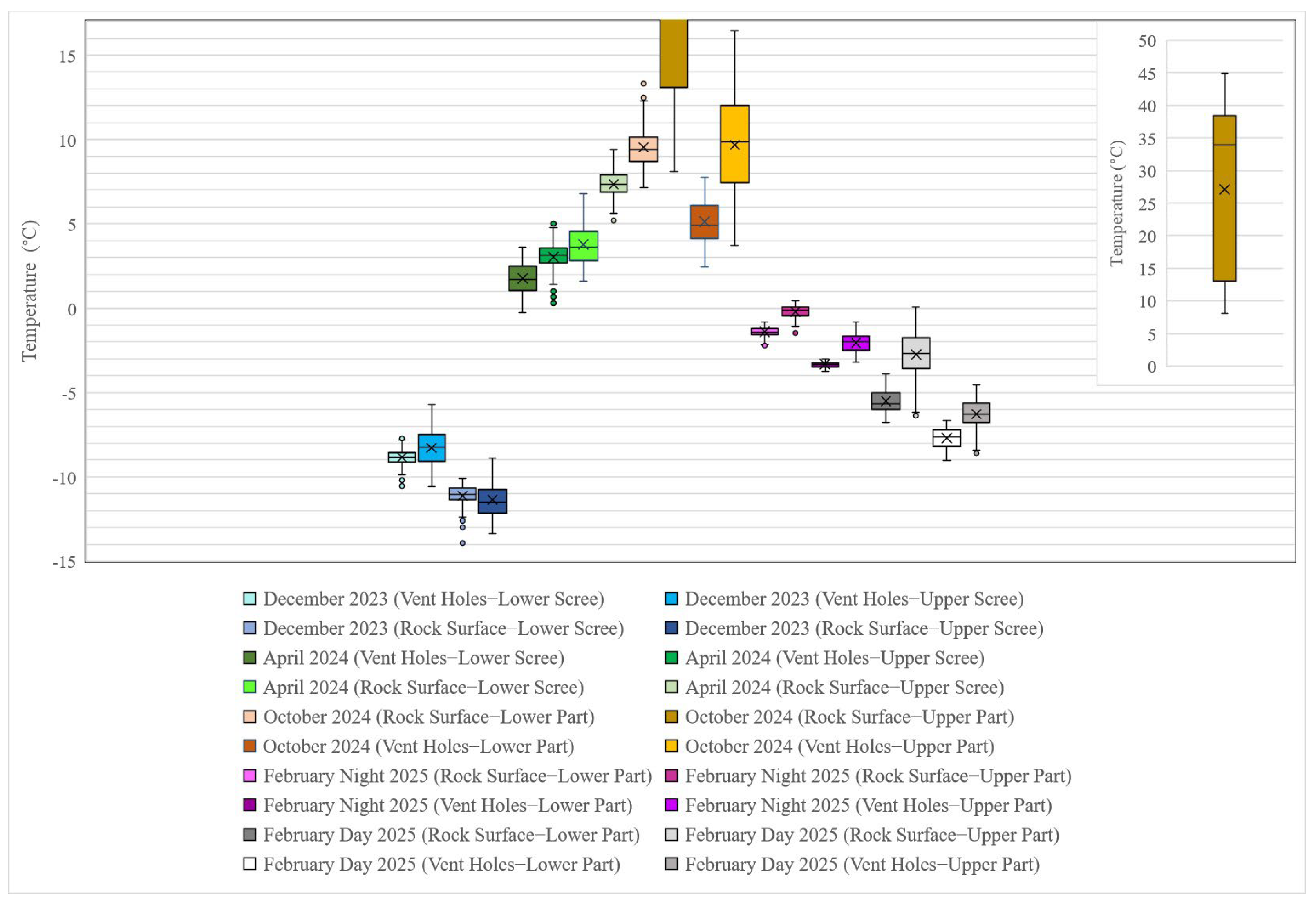
3.2. Seasonal Thermal Patterns of the Open Scree
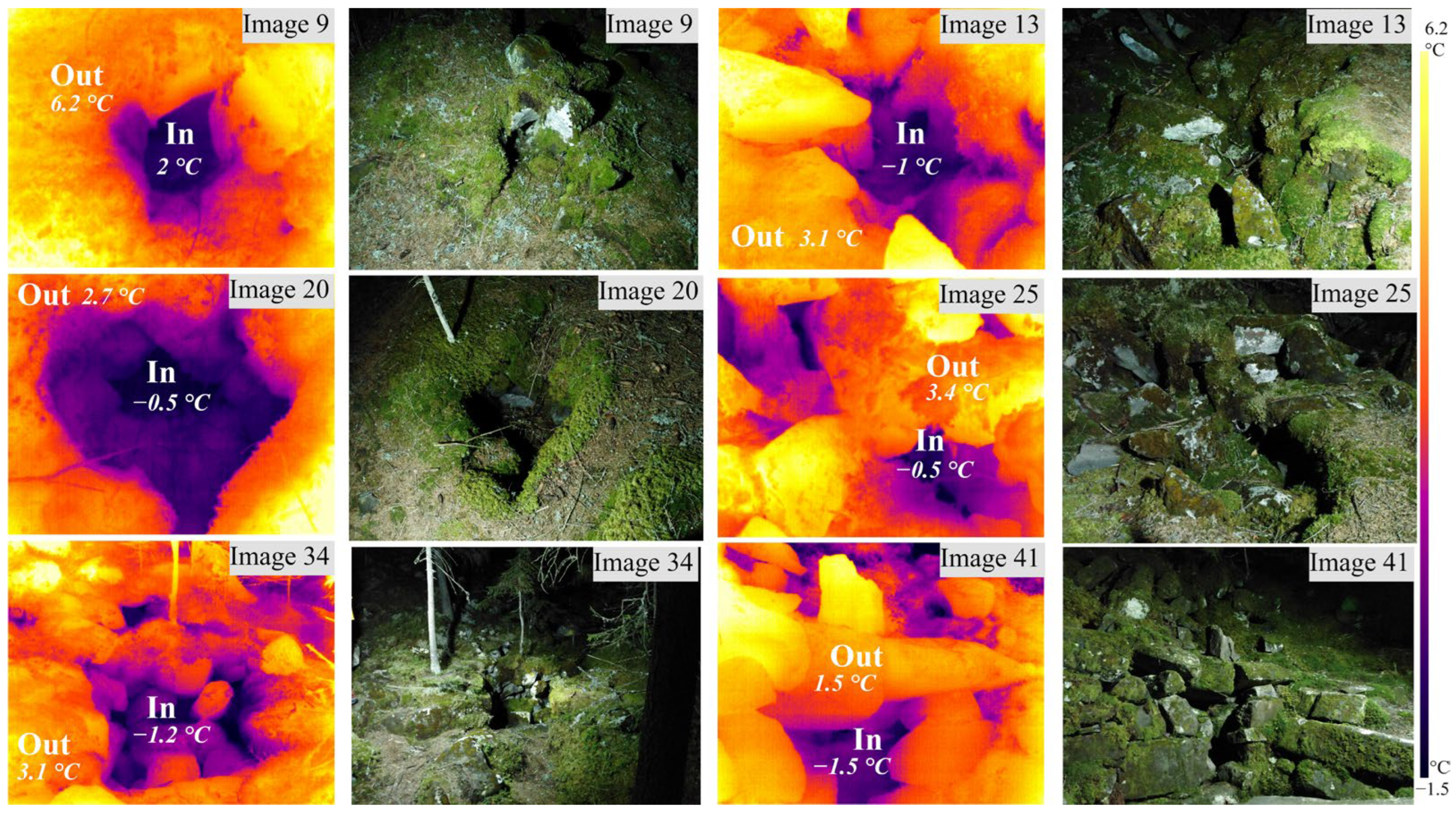
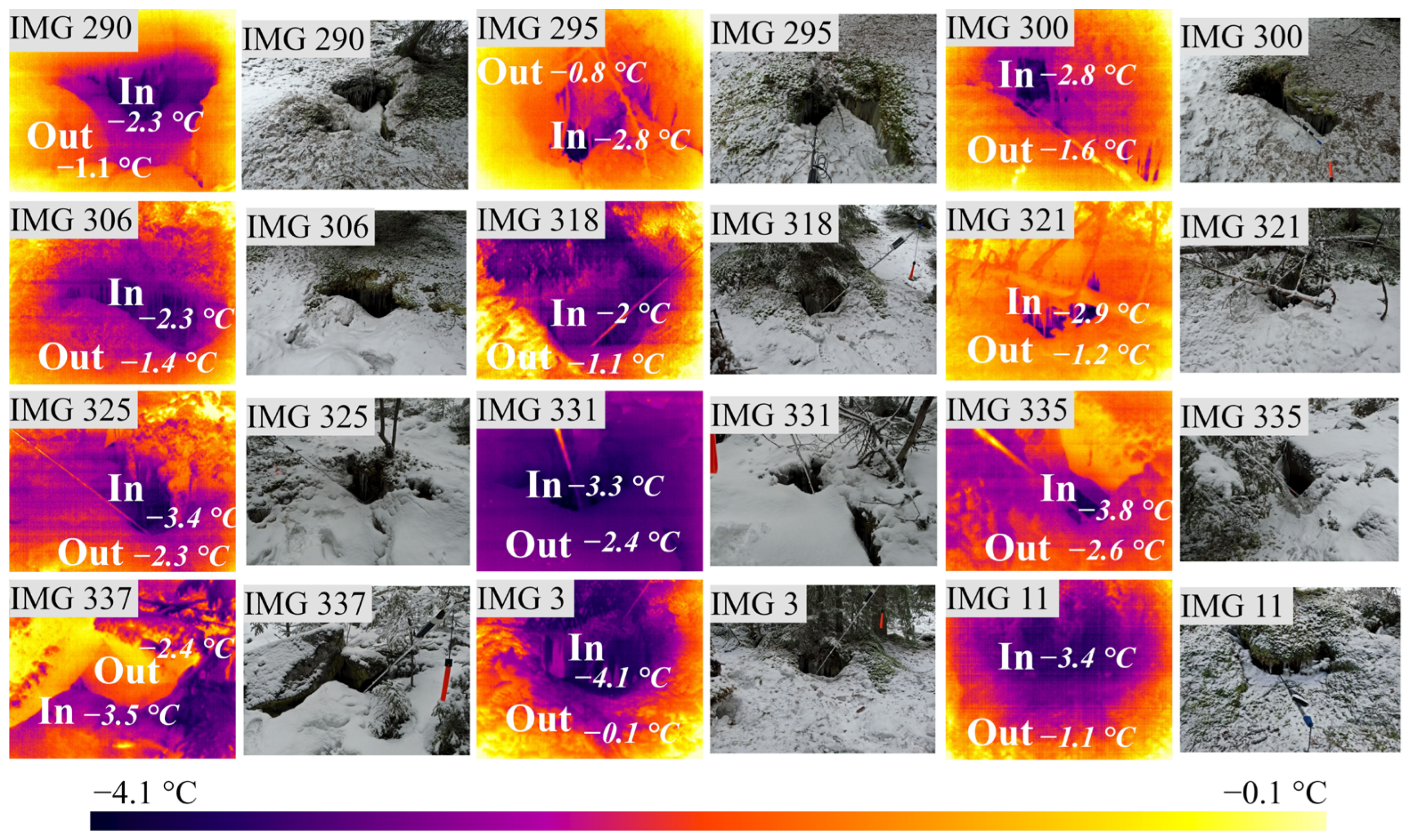
3.3. Results from the Forest Sector Imagery
4. Discussion
5. Conclusions
Supplementary Materials
Author Contributions
Funding
Data Availability Statement
Acknowledgments
Conflicts of Interest
References
- French, H.M. Periglacial Environment; Elsevier: Amsterdam, The Netherlands, 2017. [Google Scholar]
- Sawada, Y.; Ishikawa, M.; Ono, Y. Thermal regime of sporadic permafrost in a block slope on Mt. Nishi-Nupukaushinupuri, Hokkaido Island, Northern Japan. Geomorphology 2003, 52, 121–130. [Google Scholar] [CrossRef]
- Gude, M.; Dietrich, S.; Mäusbacher, R.; Hauck, C.; Molenda, R.; Růžička, V. Probable occurrence of sporadic permafrost in non-alpine scree slopes in central Europe. In Proceedings of the 8th International Conference on Permafrost, Zurich, Switzerland, 20–25 July 2003; pp. 331–336. [Google Scholar]
- Delaloye, R.; Lambiel, C. Evidence of winter ascending air circulation throughout talus slopes and rock glaciers situated in the lower belt of alpine discontinuous permafrost (Swiss Alps). Nor. Geogr. Tidsskr. 2005, 59, 194–203. [Google Scholar] [CrossRef]
- Morard, S.; Delaloye, R.; Lambiel, C. Pluriannual thermal behavior of low elevation cold talus slopes in western Switzerland. Geogr. Helv. 2010, 65, 124–134. [Google Scholar] [CrossRef]
- Stiegler, C.; Rode, M.; Sass, O.; Otto, J.C. An undercooled scree slope detected by geophysical investigations in sporadic permafrost below 1000 M ASL, central Austria. Permafr. Periglac. Process. 2014, 25, 194–207. [Google Scholar] [CrossRef]
- Popescu, R.; Vespremeanu-Stroe, A.; Onaca, A.; Vasile, M.; Cruceru, N.; Pop, O. Low-altitude permafrost research in an overcooled talus slope–rock glacier system in the Romanian Carpathians (Detunata Goală, Apuseni Mountains). Geomorphology 2017, 295, 840–854. [Google Scholar] [CrossRef]
- Wicky, J.; Hilbich, C.; Delaloye, R.; Hauck, C. Modeling the Link Between Air Convection and the Occurrence of Short-Term Permafrost in a Low-Altitude Cold Talus Slope. Permafr. Periglac. Process. 2024, 35, 202–217. [Google Scholar] [CrossRef]
- Urdea, P.; Ardelean, F.; Ardelean, M.; Onaca, O.; Berzescu, O. Glacial landscape evolution during the Holocene in the Romanian Carpathians. In European Glacial Landscapes; Palacios, D., Ed.; Elsevier: Amsterdam, The Netherlands, 2024; pp. 331–352. [Google Scholar]
- Humlum, O.; Christiansen, H.H.; Åkerman, H.J. Periglacial and Glacial Processes, 10th ed.; Elsevier: Amsterdam, The Netherlands, 2010. [Google Scholar]
- Germain, D.; Milot, J. An overcooled coarse-grained talus slope at low elevation: New insights on air circulation and environmental impacts, Cannon Cliff, New Hampshire, USA. Earth Surf. Process Landf. 2024, 49, 1705–1720. [Google Scholar] [CrossRef]
- Kneisel, C.; Hauck, C.; Mühll, D.V. Permafrost below the timberline confirmed and characterized by geoelectrical resistivity measurements, Bever Valley, eastern Swiss Alps. Permafr. Periglac. Process. 2000, 11, 295–304. [Google Scholar] [CrossRef]
- Juliussen, H.; Humlum, O. Thermal regime of openwork block fields on the mountains Elgåhogna and Sølen, central-eastern Norway. Permafr. Periglac. Process. 2008, 19, 1–18. [Google Scholar] [CrossRef]
- Colucci, R.R.; Forte, E.; Žebre, M.; Maset, E.; Zanettini, C.; Guglielmin, M. Is that a relict rock glacier? Geomorphology 2019, 330, 177–189. [Google Scholar] [CrossRef]
- Carturan, L.; Zuecco, G.; Andreotti, A.; Boaga, J.; Morino, C.; Pavoni, M.; Seppi, R.; Tolotti, M.; Zanoner, T.; Zumiani, M. Spring-water temperature suggests widespread occurrence of Alpine permafrost in pseudo-relict rock glaciers. Cryosphere 2024, 18, 5713–5733. [Google Scholar] [CrossRef]
- Wiegand, T.; Kneisel, C. Monitoring of thermal conditions and snow dynamics at periglacial block accumulations in a low mountain range in central Germany. Earth Surf. Process Landf. 2024, 49, 5321–5338. [Google Scholar] [CrossRef]
- Morard, S.; Delaloye, R.; Dorthe, J. Seasonal thermal regime of a mid-latitude ventilated debris accumulation. In Proceedings of the Ninth International Conference on Permafrost, Fairbanks, AK, USA, 29 June–3 July 2008; pp. 1233–1238. [Google Scholar]
- World Meteorological Organization. The State of the Global Climate 2020. Available online: https://public.wmo.int/en/our-mandate/climate/wmo-statement-state-of-global-climate (accessed on 27 January 2025).
- World Meteorological Organization. Guide to Instruments and Methods of Observation—Measurement of Meteorological Variables; World Meteorological Organization: Geneva, Switzerland, 2023; Volume 1, Available online: https://library.wmo.int/records/item/68695-guide-to-instruments-and-methods-of-observation?offset=3 (accessed on 27 January 2025).
- Smith, S.L.; Bonnaventure, P.P. Quantifying Surface Temperature Inversions and Their Impact on the Ground Thermal Regime at a High Arctic Site. Arct. Antarct. Alp. Res. 2017, 49, 173–185. [Google Scholar] [CrossRef]
- Tomlinson, C.J.; Chapman, L.; Thornes, J.E.; Baker, C. Remote sensing land surface temperature for meteorology and climatology: A review. Meteorol. Appl. 2011, 18, 296–306. [Google Scholar] [CrossRef]
- Pietroni, I.; Argentini, S.; Petenko, I. One Year of Surface-Based Temperature Inversions at Dome C, Antarctica. Bound. Layer Meteorol. 2014, 150, 131–151. [Google Scholar] [CrossRef]
- Gustafsson, T.; Bendz, E. Guidelines for Drone Usage in Arctic Environment-Integrating Activities for Advanced Communities. 2018. Available online: www.afconsult.com (accessed on 10 June 2024).
- Shahmoradi, J.; Talebi, E.; Roghanchi, P.; Hassanalian, M. A Comprehensive Review of Applications of Drone Technology in the Mining Industry. Drones 2020, 4, 34. [Google Scholar] [CrossRef]
- Kraaijenbrink, P.D.A.; Shea, J.M.; Litt, M.; Steiner, J.F.; Treichler, D.; Koch, I.; Immerzeel, W.W. Mapping Surface Temperatures on a Debris-Covered Glacier With an Unmanned Aerial Vehicle. Front. Earth Sci. 2018, 6, 64. [Google Scholar] [CrossRef]
- Vivaldi, V.; Bordoni, M.; Mineo, S.; Crozi, M.; Pappalardo, G.; Meisina, C. Airborne combined photogrammetry—Infrared thermography applied to landslide remote monitoring. Landslides 2023, 20, 297–313. [Google Scholar] [CrossRef]
- Sass, O.; Bauer, C.; Heil, S.; Schnepfleitner, H.; Kropf, F.; Gaisberger, C. Infrared thermography monitoring of rock faces–Potential and pitfalls. Geomorphology 2023, 439, 108837. [Google Scholar] [CrossRef]
- Ponti, S.; Girola, I.; Guglielmin, M. Thermal photogrammetry on a permafrost rock wall for the active layer monitoring. Sci. Total Environ. 2024, 917, 170391. [Google Scholar] [CrossRef]
- Urdea, P. Un permafrost de altitudine joasă la Detunata Goală (Munţii Apuseni). Rev. De Geomorfol. 2000, 2, 173–178. [Google Scholar]
- Popescu, R.; Vasile, M.; Vespremenau-Stroe, A. Chimney circulation, thermal regime and internal structure of a low altitude cold talus slope-rock glacier system (Detunata Goală, Romanian Carpathians). In Book of Abstracts: EUCOP6; Fernández-Fernández, J.M., Bonsoms, J., Garcia-Oteyza, J., Oliva, M., Eds.; Puigcerda, Spain, 2023; Available online: https://www.permafrost.org/wp-content/uploads/EUCOP6_Book_of_Abstracts.pdf (accessed on 10 June 2024).
- Oncescu, N. Geologia României; Editura Tehnică: Bucharest, Romania, 1965. [Google Scholar]
- Popescu, R. Permafrostul din Carpatii Romanesti. Studiu de Geomorfologie; Editura Universitară: Bucharest, Romania, 2021. [Google Scholar] [CrossRef]
- Wicky, J.; Hauck, C. Air convection in the Active Layer of Rock Glaciers. Front. Earth. Sci. 2020, 8, 335. [Google Scholar] [CrossRef]
- Balch, E.S. Glaciéres or Freezing Caverns; Allen, Lane & Scott: Philadelphia, PA, USA, 1900. [Google Scholar]
- Eltner, A.; Hoffmeister, D.; Kaiser, A.; Karrasch, P.; Klingbeil, L.; Stöcker, C. UAVs for the Environmental Sciences-Methods and Applications; WBG Academic: Washington, DC, USA, 2022. [Google Scholar]
- Available online: https://www.dominiondrones.com/ (accessed on 5 March 2024).
- Available online: https://geoportal.ancpi.ro/portal/apps/webappviewer/index.html?id=3f34ee5af71c400396dda574f0d53274 (accessed on 20 November 2023).
- Pereyra Irujo, G. IRimage: Open source software for processing images from infrared thermal cameras. PeerJ Comput. Sci. 2022, 8, e977. [Google Scholar] [CrossRef]
- Available online: https://github.com/gpereyrairujo/IRimage (accessed on 20 June 2024).
- Available online: https://imagej.net/licensing/ (accessed on 20 June 2024).
- Mineo, S.; Pappalardo, G. Rock Emissivity Measurement for Infrared Thermography Engineering Geological Applications. Appl. Sci. 2021, 11, 3773. [Google Scholar] [CrossRef]
- Delaloye, R. Contribution à L’étude du Pergélisol de Montagne en Zone Marginale. Ph.D. Dissertation, University of Fribourg, Fribourg, Switzerland, 2004. [Google Scholar]
- Delaloye, R.; Reynard, E.; Lambiel, C.; Marescot, L.; Monnet, R. Thermal anomaly in a cold scree slope (Creux du Van, Switzerland). In Proceedings of the 8th International Conference on Permafrost, Zurich, Switzerland, 21–25 July 2003; Phillips, M., Springman, S.M., Arenson, L.U., Eds.; A.A. Balkema Publishers: Lisse, NY, USA, 2003; pp. 175–180. [Google Scholar]
- Available online: https://www.dji.com/global/downloads/softwares/dji-dtat3 (accessed on 1 November 2024).
- Harris, S.A.; Pedersen, D.E. Thermal regimes beneath coarse blocky materials. Permafr. Periglac. Process. 1998, 9, 107–120. [Google Scholar] [CrossRef]
- Rödder, T.; Kneisel, C. Influence of snow cover and grain size on the ground thermal regime in the discontinuous permafrost zone, Swiss Alps. Geomorphology 2012, 175–176, 176–189. [Google Scholar] [CrossRef]
- Onaca, A.L.; Urdea, P.; Ardelean, A.C. Internal structure and permafrost characteristics of the rock glaciers of Southern Carpathians (Romania) assessed by geoelectrical soundings and thermal monitoring. Geogr. Ann. A Phys. Geogr. 2013, 95, 249–266. [Google Scholar] [CrossRef]
- Onaca, A.; Ardelean, A.C.; Urdea, P.; Ardelean, F.; Sirbu, F. Detection of mountain permafrost by combining conventional geophysical methods and thermal monitoring in the Retezat Mountains, Romania. Cold Reg. Sci. Technol. 2015, 119, 111–123. [Google Scholar] [CrossRef]
- Popescu, R.; Filhol, S.; Etzelmüller, B.; Vasile, M.; Pleșoianu, A.; Vîrghileanu, M.; Onaca, A.; Șandric, I.; Săvulescu, I.; Cruceru, N.; et al. Permafrost Distribution in the Southern Carpathians, Romania, Derived From Machine Learning Modeling. Permafr. Periglac. Process. 2024, 35, 243–261. [Google Scholar] [CrossRef]
- Onaca, A.; Sirbu, F.; Poncos, V.; Hilbich, C.; Strozzi, T.; Urdea, P.; Popescu, R.; Berzescu, O.; Etzelmüller, B.; Vespremeanu-Stroe, A.; et al. Slow-moving rock glaciers in marginal periglacial environment of Southern Carpathians. EGUsphere 2025, preprint. [Google Scholar] [CrossRef]
- Zacharda, M.; Gude, M.; Růžička, V. Thermal regime of three low elevation scree slopes in Central Europe. Permafr. Periglac. Process. 2007, 18, 301–308. [Google Scholar] [CrossRef]
- Kellerer-Pirklbauer, A.; Pauritsch, M.; Winkler, G. Widespread occurrence of ephemeral funnel hoarfrost and related air ventilation in coarse-grained sediments of a relict rock glacier in the Seckauer Tauern range, Austria. Geogr. Ann. A Phys. Geogr. 2015, 97, 453–471. [Google Scholar] [CrossRef]


| Statistic Type | Vent Holes/Rock Surfaces (December 23) (°C) | Temperature Diff (December 23) (°C) | Vent Holes/ Rock Surfaces (April 24) (°C) | Temperature Diff (April 24) (°C) | Vent Holes/ Rock Surfaces (February 25) (°C) | Temperature Diff (February 25) (°C) |
|---|---|---|---|---|---|---|
| Average | −6.03/−3.88 | −2.15 | 0.08/3.86 | 3.78 | −2.91/−1.69 | −1.22 |
| Median | −5.8/−4.25 | 1.59 | −0.4/3.4 | 3.8 | −1.69/−1.5 | −0.19 |
| Minimum | −9.9/−7.4 | 2.5 | −3.6/0.2 | −3.8 | −4.2/−2.9 | 1.3 |
| Maximum | −2.6/−0.5 | 3.1 | 4.9/9.6 | 4.7 | −1.6/−0.4 | 2 |
| StDev | 2.39/2.17 | −0.22 | 1.72/2.03 | 0.31 | 0.55/0.63 | 0.08 |
Disclaimer/Publisher’s Note: The statements, opinions and data contained in all publications are solely those of the individual author(s) and contributor(s) and not of MDPI and/or the editor(s). MDPI and/or the editor(s) disclaim responsibility for any injury to people or property resulting from any ideas, methods, instructions or products referred to in the content. |
© 2025 by the authors. Licensee MDPI, Basel, Switzerland. This article is an open access article distributed under the terms and conditions of the Creative Commons Attribution (CC BY) license (https://creativecommons.org/licenses/by/4.0/).
Share and Cite
Ioniță, A.; Lopătiță, I.; Urdea, P.; Berzescu, O.; Onaca, A. Low-Altitude, Overcooled Scree Slope: Insights into Temperature Distribution Using High-Resolution Thermal Imagery in the Romanian Carpathians. Land 2025, 14, 607. https://doi.org/10.3390/land14030607
Ioniță A, Lopătiță I, Urdea P, Berzescu O, Onaca A. Low-Altitude, Overcooled Scree Slope: Insights into Temperature Distribution Using High-Resolution Thermal Imagery in the Romanian Carpathians. Land. 2025; 14(3):607. https://doi.org/10.3390/land14030607
Chicago/Turabian StyleIoniță, Andrei, Iosif Lopătiță, Petru Urdea, Oana Berzescu, and Alexandru Onaca. 2025. "Low-Altitude, Overcooled Scree Slope: Insights into Temperature Distribution Using High-Resolution Thermal Imagery in the Romanian Carpathians" Land 14, no. 3: 607. https://doi.org/10.3390/land14030607
APA StyleIoniță, A., Lopătiță, I., Urdea, P., Berzescu, O., & Onaca, A. (2025). Low-Altitude, Overcooled Scree Slope: Insights into Temperature Distribution Using High-Resolution Thermal Imagery in the Romanian Carpathians. Land, 14(3), 607. https://doi.org/10.3390/land14030607