Article

Embedding Ordinal Optimization into Tree–Seed Algorithm for Solving the Probabilistic Constrained Simulation Optimization Problems

by
Shih-Cheng Horng
1,* and
Shieh-Shing Lin
2
1
Department of Computer Science & Information Engineering, Chaoyang University of Technology, Taichung 41349, Taiwan
2
Department of Electrical Engineering, St. John’s University, New Taipei City 25135, Taiwan
*
Author to whom correspondence should be addressed.
Appl. Sci. 2018, 8(11), 2153; https://doi.org/10.3390/app8112153
Submission received: 19 October 2018 / Revised: 25 October 2018 / Accepted: 29 October 2018 / Published: 3 November 2018

Abstract

:
Probabilistic constrained simulation optimization problems (PCSOP) are concerned with allocating limited resources to achieve a stochastic objective function subject to a probabilistic inequality constraint. The PCSOP are NP-hard problems whose goal is to find optimal solutions using simulation in a large search space. An efficient “Ordinal Optimization (OO)” theory has been utilized to solve NP-hard problems for determining an outstanding solution in a reasonable amount of time. OO theory to solve NP-hard problems is an effective method, but the probabilistic inequality constraint will greatly decrease the effectiveness and efficiency. In this work, a method that embeds ordinal optimization (OO) into tree–seed algorithm (TSA) (OOTSA) is firstly proposed for solving the PCSOP. The OOTSA method consists of three modules: surrogate model, exploration and exploitation. Then, the proposed OOTSA approach is applied to minimize the expected lead time of semi-finished products in a pull-type production system, which is formulated as a PCSOP that comprises a well-defined search space. Test results obtained by the OOTSA are compared with the results obtained by three heuristic approaches. Simulation results demonstrate that the OOTSA method yields an outstanding solution of much higher computing efficiency with much higher quality than three heuristic approaches.

Graphical Abstract

1. Introduction

The probabilistic constrained simulation optimization problems (PCSOP) are concerned with allocating limited resources to achieve a stochastic objective function subject to a probabilistic inequality constraint. The performance of the PCSOP is evaluated by simulations, which may be a complex evaluation in a real-world physical system or a simple computer based mathematical model [1]. Such problems occur in almost all fields of automatic production, such as the network type flow line production system, buffer resource allocation, periodic review inventory system, as well as many industrial managements, including facility-sizing of factory and strategic location of semi-finished products in a pull-type production system. The goal of PCSOP is to search for the optimal design variables to reach desired performance subject to a probabilistic inequality constraint. The PCSOP belong to the class of NP-hard problems [2] for which most likely no polynomial time optimization method exists. In practice, the large search space makes the considered problem more difficult to determine an optimal design variable using classical optimization techniques in a short computational time.
There are many methods proved to be interesting in solving the NP-hard problems, such as the evolutionary algorithms (EA) [3], gradient search methods [4], heuristic methods [5], and swarm intelligence (SI) [6]. EA [3] are stochastic optimization approaches based on the biological evolution metaphor, which utilize the “survival of the fittest” to produce successively superior approximations to a design variable. Three main types of EA have been developed: evolution strategies (ES), evolutionary programming (EP), and genetic algorithms (GA). However, EA are usually computationally intensive and do not offer an absolute guarantee of the global optimality. The gradient search methods [4], such as conjugated gradient and steepest descent method, tends to converge very slowly and can easily get trapped in local minimum. The heuristic methods [5], such as Tabu search (TS) and simulated annealing (SA), have the capability of finding global optimal solution. However, the quality of optimal solution is highly dependent on fine-tuning of parameters.
SI [6] is an emerging field of biologically-inspired artificial intelligence based on the behavioral models of social insects such as colonies of ants, bees, schools of fish and flocks of birds. Some of the recent established SI methods include elephant herding optimization (EHO), bacteria foraging optimization (BFO), social spider optimization (SSO), crow search algorithm (CSA), bat algorithm (BA) and tree–seed algorithm (TSA) [7]. Most SI methods require only objective values and accomplish a proper balance between exploration and exploitation. However, there are still a number of significant barriers and technical hurdles to overcome [8].
The following three issues make the PCSOP difficult to solve: (i) the search space is large; (ii) evaluating performance is time-consuming; and (iii) single probabilistic inequality constraint must be satisfied. The purpose of this paper is to resolve the PCSOP efficiently and effectively. To overcome the three issues simultaneously, an ordinal optimization (OO) theory [9] attempts to quickly determine a good enough solution. OO is used to supplement available optimization methods, but is not itself an optimization approach. OO theory considers order rather than value to reduce the computational complexity of optimization process, and guarantees a high probability that the obtained solution is good enough. In the OO theory, the first step is to create a selected subset by rapidly evaluating all solutions using a rough evaluation. A rough evaluation estimates performance with high tolerance of modeling noise. OO theory indicates that the order of solutions is nearly kept even though they are assessed by a rough evaluation [9]. Next, an outstanding subset is constructed from the selected subset. Finally, each solution in the outstanding subset is assessed using a precise evaluation. A precise evaluation is one that can yield exact estimates of performance. The one with the best performance in the outstanding subset is the good enough solution. The OO theory has been successfully used in various applications, such as the flow line system [10], assemble-to-order systems [11], and network-type production line [12].
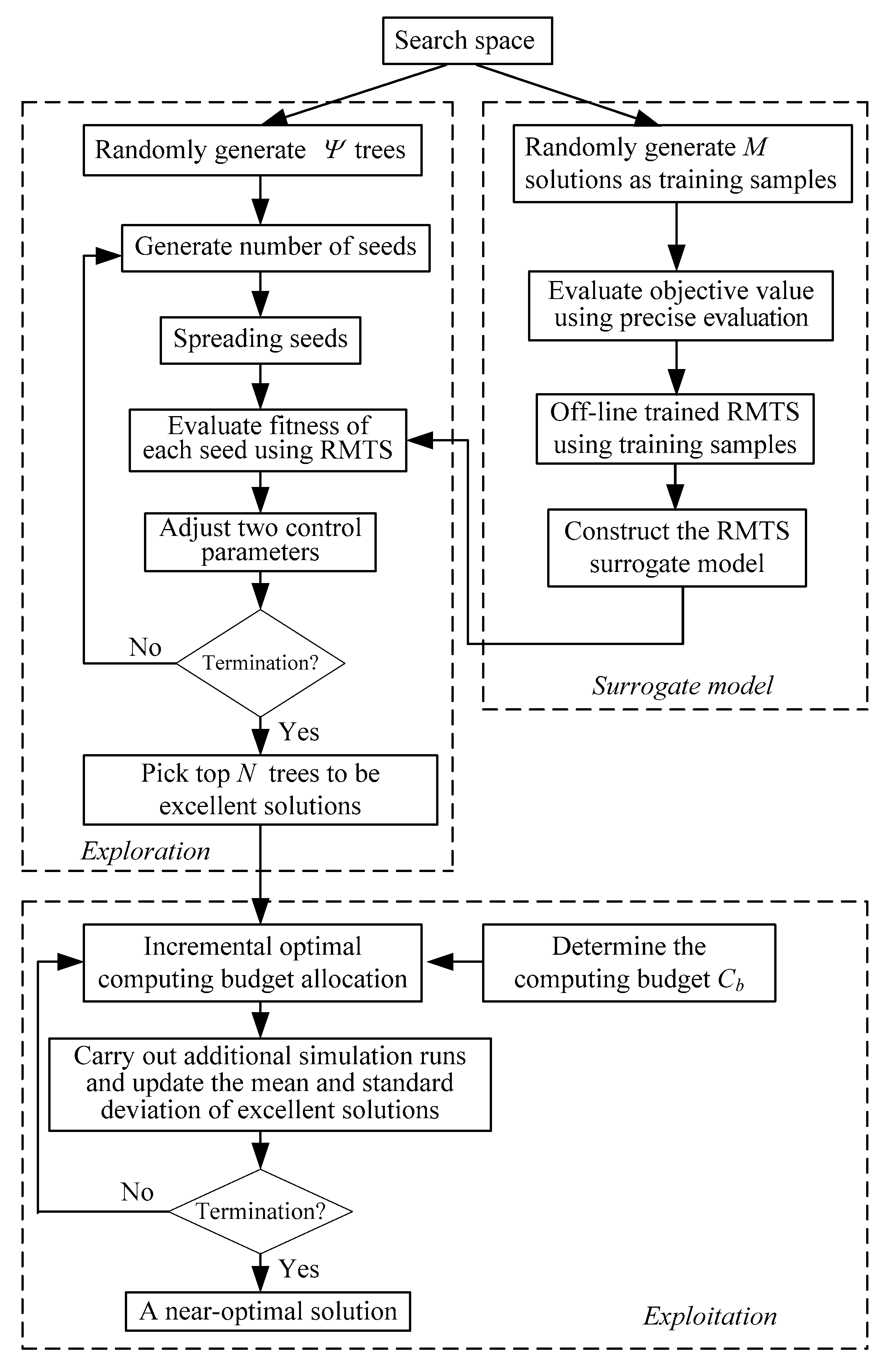
To reduce the computing time of PCSOP, a method that embeds ordinal optimization (OO) into tree–seed algorithm (TSA) [13,14,15,16] (OOTSA) is proposed to determine a near-optimal solution in a short computational time. The OOTSA method contains three modules: surrogate model, exploration and exploitation. Firstly, the regularized minimal-energy tensor-product splines (RMTS) [17] is utilized as a surrogate model to approximately evaluate a solution. Secondly, an improved tree–seed algorithm (ITSA) is proceeded to choose N outstanding solutions from the large search space. Finally, an incremental optimal computing budget allocation (IOCBA) technique is employed to determine the optimal solution from the N outstanding solutions. These three modules drastically diminish the computing effort of PCSOP.
To test the performance of the proposed OOTSA approach, it is employed to a pull-type production system. The pull-type production system is formulated as a PCSOP that is comprised a huge search space. The goal of a pull-type production system is to determine the optimal work-in-process inventory for minimizing the expected lead time while satisfying a tolerable service level. The first contribution of this paper is to propose an OOTSA approach for a general PCSOP that is lack of structural information to determine a near-optimal solution in a short computational time. The second contribution is to employ the proposed approach to minimize the expected lead time of a pull-type production system such that the work-in-process inventory is optimized.
This paper contains five sections. After this Introduction, Section 2 explains the proposed OOTSA to search for an outstanding solution of a general PCSOP. Section 3 formulates the pull-type production system as a PCSOP and discusses the application of the proposed OOTSA for optimization of this PCSOP. Finally, Section 4 and Section 5 are the results of this research and the conclusion, respectively.

2. Embedded Ordinal Optimization into Tree–Seed Algorithm

2.1. Mathematical Formulation

The mathematical formulation of a general PCSOP is described as follows [1].
min   E [ f ( x ) ]  
subject   to   P [ g ( x ) 0 ] θ  
V x U  
where x = [ x 1 , , x n ] T is an n-dimensional decision vector, V = [ V 1 , , V n ] T denotes the vector of lower bound, U = [ U 1 , , U n ] T represents the vector of upper bound, f ( x ) is the objective function, E [ f ( x ) ] represents the expected objective value, P [ g ( x ) 0 ] denotes the probability of the satisfaction of the constraint g ( x ) 0 , and θ is a fixed probability level lying in a range [0,1].
Multiple simulation runs are carried out to obtain an accurate estimate of the expected objective value and probability. In practice, it is impossible to run simulations infinitely long. An alternative way of approximating the expected objective value and probability is to use the sample mean as follows.
f ¯ ( x ) = 1 L j = 1 L f j ( x )  
p ( x ) = 1 L j = 1 L y j  
where L represents the amount of simulation runs, f j ( x ) denotes the objective value of the j th simulation run, y j = 0 indicates that the constraint g ( x ) 0 is not satisfied, and y j = 1 denotes that a satisfaction of the constraint. The sample mean of f ¯ ( x ) achieves a better approximation of E [ f ( x ) ] when L increases.
Because the probabilistic constraint is a soft constraint, a quadratic penalty function [18] is used to convert the constrained optimization problem into an unconstrained optimization problem.
min   F ( x ) = λ × f ¯ ( x ) + ( 1 λ ) × P F ( x )  
where λ ( 0 , 1 ) is a penalty weight, F ( x ) is a weighted objective value, and P F ( x ) indicates a quadratic penalty function as follows.
P F ( x ) = { 0 ,    i f   p ( x ) θ , 10 4 × ( θ p ( x ) ) 2 , e l s e .  
There is a sharp jump in the penalty function to guarantee that the probability does not exceed the fixed probability level. Let L s denote the large enough of simulation runs, and the precise evaluation of Equation (6) is defined by using L = L s . For simplicity, we define F s ( x ) as the objective value of Equation (6) obtained by precise evaluation for x .
As pointed out by the OO theory [9], order of a solution is probably preserved even evaluating by a surrogate model. To select N outstanding solutions in an exceptionally short period of time, we need to establish a surrogate model which can evaluate a solution very fast and utilize an optimization technique assisted by the surrogate model. The RMTS [17] is adopted as a surrogate model, and the ITSA is the optimization technique.

2.2. RMTS Surrogate Model

Surrogate models have been used in wide fields and applications, including time series prediction, system control, classification, curve fitting and function approximation [19]. Surrogate models are used to approximate a function according to training samples and can be used to predict the value of new sampling points [20]. Surrogate models can be classified as regression or interpolation [21]. Interpolation models match the function value at each training sample, while regression models do not. Regression techniques smoothly approximate noisy data, such as the artificial neural networks (ANN), extreme learning machine (ELM), multivariate adaptive regression splines (MARS), polynomials, and support vector regression (SVR). Interpolation techniques try to accurately suit non-noisy data, such as the kriging, radial basis functions (RBF), local polynomial interpolation (LPI), in-verse distance weighting (IDW), and RMTS. Among them, RMTS is not easily influenced by training failure.
In this research, a surrogate model based on RMTS is developed to evaluate a solution very fast [17]. The prediction output of RMTS is expressed as a linear combination of basis functions with pre-computed coefficients obtained from training. The key point of RMTS is that the number of basis functions is not required to be closely related to the number of training samples. The energy minimization and regularization are used in RMTS to increase accuracy with unstructured and small datasets. When large datasets are available, the accuracy of RMTS is higher than other interpolation methods.
The structure of an RMTS is shown in Figure 1. The training data patterns for RMTS are ( x i , F s ( x i ) ), i = 1 , , M , where x i and F s ( x i ) are the decision vector and the corresponding objective value evaluated by precise evaluation, respectively. The goal of RMTS is to determine a function F R M T S ( x ) to predict approximately the desired outputs F s ( x ) . The general model of RMTS is depicted as follows.
F R M T S ( x ) = i = 1 B ω i b i ( x )  
where x denotes the decision vector, F R M T S ( x ) is the prediction output, B is the number of basis functions, ω i denotes the coefficient of the multivariate spline, and b i ( x ) is the ith basis function. For adjacent elements, the values and derivatives are continuous. In matrix notation, the general model is
F R M T S ( x ) = B ( x ) w  
where w = [ ω 1 , , ω B ] T is the vector of spline coefficients, and B ( x ) = [ b 1 ( x ) , , b B ( x ) ] is the vector mapping the spline coefficients to the prediction output. RMTS obtains the coefficients of the splines, w, by solving an energy minimization problem with the constraint that the splines must pass through the training data patterns. The objective function of the energy minimization problem consists of the following three terms: the first term containing the second derivatives of the splines, the second term for regularization, and the last term representing the approximation error for the training data.
min w 1 2 w T H w + 1 2 σ w T w + 1 2 ρ i = 1 M ( B ( x i ) w F s ( x i ) ) 2  
where x i denotes the decision vector for the ith training data pattern, F s ( x i ) represents the output value of x i , H is the matrix containing the second derivatives, B(xi) is the vector mapping the spline coefficients to the ith training output, σ is the weight of the term penalizing the norm of the spline coefficients, and ρ is the weight on gradient training data.
Treating the decision vector x as an input, the output of RMTS F R M T S ( x ) is desired to approximately estimate F s ( x ) . After training the RMTS off-line, the value of F R M T S ( x ) for any x can be obtained by performing simple arithmetic operations.

2.3. Improved Tree–Seed Algorithm

Next, we can efficiently select N outstanding solutions from search space using optimization approaches assisted by the RMTS surrogate model. Because the TSA iteratively aims at improving the candidate solutions, it would be best suited for our needs. The advantages of TSA include ease of implementation, only a few parameters need to be adjusted, tactical interplay between searching diversification and intensification, quick convergence and high efficiency [14]. TSA is inspired from the relation between trees and seeds, which simulates the growth cycles of trees and seeds on a land [16]. The trees and their seeds correspond to the possible solution while the land indicates the search space of the optimization problems. At the beginning of the iteration, the trees are sowed to the land. Then, a pre-defined number of seeds for each tree are generated during the search process. If the performance of the best seed is better than its tree, the best seed is added to the stand and its tree is removed from the stand. This search process is performed until a required number of iteration is met.
The following is a description of the developed ITSA. Firstly, an initial tree population is generated. Each tree is randomly assigned an initial position. Secondly, a new seed is spread from a tree, either the best tree location of another tree location is considered with its own location. The first scheme uses the best tree to provide a speed convergence, and the second one uses the randomly selected tree to explore spacious regions on the search space. The key point is which tree location will be chosen to generate a new seed location. This selection depend on the search tendency (ST), which varies within a range of 0–1. The number of seeds generated by a tree can be more than one, which depends on the seed produced rate (SPR). More seeds improve the global search capability but require more computing time. This iterative process is performed until the pre-defined number of iterations has been reached.
The ITSA has two control factors: ST and SPR. The intensification and diversification of the ITSA are mainly controlled by the ST. A large ST causes a speed convergence and powerful local search, while a small ST provides a powerful global search but slow convergence. When the ST is decreased, the ability of local search decreases and the ITSA trends to perform the global search. When the ST is increased, the ITSA tends to conduct the local search around a local region. Similarly, a lower SPR tends to local search, while a higher SPR leads to global search.
The algorithmic notations used in the ITSA are described as follows. Ψ denotes the size of tree population; k max denotes the pre-defined number of iterations; S T k [ S T min , S T max ] is the ST at iteration k, where S T max and S T min represent the maximum and minimum of ST, respectively; and γ k [ γ min , γ max ] is the SPR at iteration k, where γ max and γ min denote the maximum and minimum of SPR, respectively. The position of the ith tree and the jth seed at iteration k in an n-dimensional space is represented by x i k = [ x i , 1 k , , x i , n k ] T and s j k = [ s j , 1 k , , s j , n k ] T , respectively.
According to the analysis mentioned above, the ITSA can be summarized as follows.
Algorithm 1: The ITSA
Step 1: Define parameters
Define the values of Ψ , k max , S T min , S T max , γ min , γ max , and set S T 0 = S T min , γ 0 = γ max , k = 0 , where k denotes the iteration index.
Step 2: Initialization
(a) Initialize the first population of Ψ trees with positions x i 0 as follows.
x i , j 0 = V j + r a n d [ 0 , 1 ] × ( U j V j ) ,   i = 1 , , Ψ ,   j = 1 , , n .
  where r a n d [ 0 , 1 ] is a random number in the interval [0,1], Uj is the upper bound, and Vj is the lower bound.
(b) Evaluate the approximate fitness F RMTS ( x i 0 ) of each tree assisted by the RMTS, i = 1 , , Ψ .
(c) Rank these Ψ trees based on their fitness from lowest to highest, then determine the best-so-far tree x = [ x 1 , , x n ] T .
Step 3: Generate the number of seeds for each tree
i k = Ψ × ( γ min + ( γ k γ min ) × r a n d [ 0 , 1 ] ) + 1 ,   i = 1 , , Ψ .
  where indicates the rounding function, which rounds to the next lower integral value.
Step 4: Spreading seeds
(a) Generate positions of all seeds
  For i = 1 , , Ψ , do
  For l = 1 , , i k , do
  For j = 1 , , n , do
    If r a n d [ 0 , 1 ] < S T k
s l , j k = x i , j k + r a n d [ 1 , 1 ] × ( x j x r , j k )
    Else
s l , j k = x i , j k + r a n d [ 1 , 1 ] × ( x i , j k x r , j k )
where x j denotes the jth position of best-so-far tree, r a n d [ 1 , 1 ] is a random number in the interval [−1,1], and i r . If s l , j k < V j , set s l , j k = V j , and if s l , j k > U j , set s l , j k = U j .
(b) Evaluate the approximate fitness F RMTS ( s l k ) for each seed produced from the ith tree assisted by the RMTS, l = 1 , , i k .
(c) Rank these i k seeds based on their fitness from lowest to highest, then select the best seed h i k . Apply the greedy choice among h i k and x i k . If F RMTS ( h i k ) < F RMTS ( x i k ) , then set x i k + 1 = h i k ; else, set x i k + 1 = x i k .
Step 5: Update control parameters
S T k + 1 = S T min + ( S T max S T min ) × exp ( 1 k max k + 1 )
γ k + 1 = γ min + ( γ max γ min ) × exp ( ln ( γ min γ max ) 2 × k + 1 k max )
Step 6: Update best-so-far tree
  Apply the greedy choice among x i k + 1 and x , i = 1 , , Ψ . If F RMTS ( x i k + 1 ) < F RMTS ( x ) , then set x = x i k + 1 .
Step 7: Termination
  If k k max , stop; otherwise, set k = k + 1 and go to Step 3.
The ITSA uses the following two conditions to determine when to stop. The first one stops when the best-so-far fitness does not change during the last given iterations, and the other stops when the number of iterations reaches a required number of iterations. In this paper, the ITSA stops when the number of iterations reaches k max iterations. The final Ψ trees are ranked based on their objective values after termination. Accordingly, the top N trees are selected to be the N outstanding solutions.

2.4. Incremental Optimal Computing Budget Allocation

Starting from the N outstanding solutions, we continue to search for the best solution by the IOCBA technique. The IOCBA technique can incrementally decide the computing efforts for promising solutions. The key criteria of the IOCBA is providing less computing effort on most mediocre solutions and more on few excellent solutions. Focusing on only few excellent solutions can decrease computation time and reduce the variances of these excellent solutions.
By calculating the means and standard deviations of objective value resulted from the N outstanding solutions, we can decide the additional simulation runs to spend more computing effort for excellent solutions. Let C b represent the available computing budget, and L i denote the amount of simulation runs assigned to the i th solution. The initial amount of simulation runs is L 0 , and the computing budget is increased by a pre-specified Δ in every iteration. The purpose of the IOCBA is to optimally allocate C b to L 1 , L 2 , …, L N such that L 1 + L 2 + + L N = C b ; meanwhile, the probability of obtaining the best solution is maximized. The available computing budget C b is defined as C b = N × L s s , where L s = 10 4 is the amount of simulation runs utilized in precise evaluation and s indicates a reduction factor of computing time which can be found by the OCBA theorem [22].
To decrease the computational complexity of the original OCBA, an IOCBA technique is presented in this section. The original OCBA needs to carry out all simulation runs to obtain the means and standard deviations of cumulative amount of simulation runs. The IOCBA requires only the means and standard deviations of additional amount of simulation runs to obtain the means and standard deviations of cumulative amount of simulation runs. The step-wise procedure for the IOCBA technique is described in Algorithm 2.
Algorithm 2: The IOCBA
Step 1. Define the value of L 0 and set l = 0 , L 1 0 = L 0 ,…, L N 0 = L 0 . Determine the value of C b = N × L s s .
Step 2. If i = 1 N L i l C b , terminate and select the best solution x with minimum objective value; else, go to Step 3.
Step 3. Increase a pre-specified computing budget Δ to i = 1 N L i l , and calculate the new number of simulation runs by
L j l + 1 = ( i = 1 N L i l + Δ ) × α j l / ( α b l + i = 1 , i b N α i l )
L b l + 1 = α b l α j l × L j l + 1
L i l + 1 = α i l α j l × L j l + 1
for all i j b , where α i l α j l = ( δ i l × ( F ¯ b l F ¯ j l ) δ j l × ( F ¯ b l F ¯ i l ) ) 2 , α b l = δ b l i = 1 , i b N ( α i l δ i l ) 2 , F ¯ i l = 1 L i l h = 1 L i l F h ( x i ) , δ i l = 1 L i l h = 1 F i l ( F h ( x i ) F ¯ i l ) 2 , x i is the i th solution, F h ( x i ) is the objective value of x i at the h th simulation run, and b = arg   min i F ¯ i l .
Step 4. Carry out additional number of simulation runs, i.e., max [ 0 , L i l + 1 L i l ] , on the i th promising solution, then compute the means F ^ i l + 1 and standard deviations δ ^ i l + 1 of those additional number of simulation runs by
F ^ i l + 1 = 1 ( L i l + 1 L i l ) h = L i l + 1 L i l + 1 F h ( x i )
δ ^ i l + 1 = 1 ( L i l + 1 L i l ) h = L i l + 1 L i l + 1 ( F h ( x i ) F ^ i l + 1 ) 2
respectively.
Step 5. Compute the means F ¯ i l + 1 and standard deviations δ i l + 1 of cumulative amount of simulation runs for the i th promising solution by
F ¯ i l + 1 = 1 L i l + 1 ( L i l × F ¯ i l + ( L i l + 1 L i l ) × F ^ i l + 1 )
δ i l + 1 = 1 ( L i l + 1 1 ) × ( L i l ( F ¯ i l ) 2 + ( L i l 1 ) ( δ i l ) 2 + ( L i l + 1 L i l ) ( F ^ i l + 1 ) 2 + ( L i l + 1 L i l 1 ) ( δ ^ i l + 1 ) 2 L i l + 1 ( F ^ i l + 1 ) 2 )
respectively. Set l = l + 1 and go to Step 2.

2.5. The Proposed OOTSA Approach

Figure 2 shows the flow chart of the proposed OOTSA approach. The proposed OOTSA approach is presented as follows (Algorithm 3).
Algorithm 3: The OOTSA
Step 1:
Define the values of M , Ψ , S T min , S T max , γ min , γ max , k max , N , L s , L 0 , and Δ .
Step 2:
Randomly generate M x ’s and calculate F s ( x ) for each x , then apply these M input–output pairs, ( x , F s ( x ) ), to train the RMTS.
Step 3:
Randomly generate Ψ x ’s as the initial tree population and employ Algorithm 1 to these trees assisted by RMTS. After Algorithm 1 terminates, rank the Ψ x ’s based on their approximate fitness F RMTS ( x ) from smallest to largest and choose the prior N x ’s to be the N outstanding solutions.
Step 4:
Apply Algorithm 2 to the N outstanding solutions and determine the best x , and this one is the near-optimal solution.

3. Application to Pull-Type Production System

3.1. Pull-Type Production System

In some manufacturing environment, various products are made from the same raw material in many stages of manufacturing processes. Some intermediate states of semi-finished products may be shared by some product family members. A pull-type production system is a lean manufacturing strategy used to reduce waste in the production process [23,24]. Since components are just replaced once after they were entirely consumed in the manufacturing process, manufacturers will only supply enough products to fulfill customer’s demands. Thus, all resources of the company are used to produce components which can be sold immediately and obtain a benefit. A pull-type production system starts with the order of customers, then it works backwards and adopts visual signals to facilitate operation in each previous step of the production process. The product is pulled through the production sequence based on the demands of consumer.
Pull-type production systems are designed to respond quickly to the demand change. The downstream machines pull the production from the upstream ones based on the demands created at their output buffers. Some kinds of message are sent to the upstream machines to indicate the demand for a particular component. When production stages do not need a specified resource, locating manufacturing equipment at essential stages and processing parts ahead of time can reduce the lead time using a low work-in-process level. After each operation, the product becomes a specific state that is closer to its final state. The closer the product is to its final shape, the shorter the lead time needs to produce it to a finished product. Nevertheless, when the product becomes closer toward its final shape, its flexibility to transform into a comprehensive final products is decreased. Suppose the demand of final products is uncertain, a good compromise between the service levels and lead times could be accomplished if inventories of semi-finished products were held in intermediate stages. If the production system is operated in a pull-type environment, this consideration will obtain a better result.
The goal of pull-type production system is to find the optimum work-in-process inventory for minimizing the average lead time as well as: (i) satisfying uncertain demands; (ii) maintaining the inventory levels at desirable values; and (iii) keeping a tolerable service level [25]. However, the considered problem is obviously more complex since the resources are shared at several stages of production. When stages need more rare resources to be supplied with more levels of semi-finished products, appropriately allocating the work-in-process inventories is required. Because each operation must share specified resource with other activities, it is difficult for existing optimization approaches to determine an optimal solution quickly. Furthermore, the probabilistic inequality constraint of pull-type production system significantly influences the efficiency and effectiveness during the search processes. In this section, we focus on the following two subjects: (i) convert the pull-type production system to a PCSOP; and (ii) apply the OOTSA approach to determine the optimal in-process inventories for minimizing the average lead time and maintaining an acceptable service level.

3.2. Mathematical Formulation

Consider a production system Q = (D, E) has the set of nodes D = {1, 2, …, n}. There are K different final products and m machines MC1, MC2,…, MCm. Each arc represents the transformation from one intermediate product to another and each node in D denotes a state of the product. Every transforming process uses one of the machines. Orders of the K final products are arrived at random intervals, and processing times of the m machines are also random with specified distributions. The time horizon is defined as H. The available number of raw material is equal to the expected value of the total demand for K final products.
Figure 3 shows an example of three product pull-type production system. There are two stages and each process is performed by one machine of either MC1 or MC2. Orders for the products may arrive in batches from any of the final nodes. If finished products are ready at final nodes, orders are fulfilled immediately. If no product is ready, a set of orders is delivered to some supplying nodes according to the workloads on machines. The workload is defined as the time used to produce the products which are waiting in the queue. A tally is kept on the work which is already appointed but not yet finished. For example, if an order arrives to node 5, it can be either fulfilled by semi-finished products at node 3 using MC1 through process “3-5” or by those at node 2 using MC2 through process “2-5”. According to the workloads on these two machines, the production will be allocated to the machine with light load. Ties can be broken arbitrarily.
To reduce the average lead time, all intermediate products can be processed in advanced. However, if there are too many raw materials being tied up in other products, some demands will not be satisfied. Thus, the goal of production system is to minimize the expected lead time as well as keeping a tolerable service level with high probability. Because the selections of machines, supplying nodes, and demanding nodes are not unique, the following three assumptions are used to decide the priority: (i) When a process “a-b” enters the queue of machine MCk, the machine is reserved. The machine MCk cannot begin any new arrival process until process “a-b” is finished, even if it has to be idle until node a becomes available. (ii) The processing time of any product in a queue is known. Thus, each machine can determine the total workload. (iii) If a demand can be fulfilled by different supplying nodes on different machines, the machine with the minimum workload is chosen.
The pull-type production system can be formulated as the following PCSOP.
min   E [ f ( x ) ]  
subject   to   P ( g ( x ) b ) 1 α  
V x U  
where x = [ x 1 , , x n ] T is the decision vector, xi is the levels of work-in-process inventory at node i (i.e., the amounts of intermediate products to be processed ahead of time), V = [ V 1 , , V n ] T denotes the vector of lower bound, U = [ U 1 , , U n ] T is the upper bound vector, E [ f ( x ) ] represents the expected lead time of work-in-process inventories x , g denotes the service level, b is a pre-specified acceptable service level, P ( g ( x ) b ) denotes the probability of the acceptable risk, and α denotes the risk which violates the acceptable service level.
Based on the above terminologies, we can reformulate the PCSOP as follows.
min   1 L j = 1 L f j ( x )  
subject   to   1 L j = 1 L y j 1 α ,
y j { 0 , 1 } ,   j = 1 , , L .
V x U .
where L is the total amount of simulation runs and f j ( x ) denotes the objective value of the j th simulation run. The inequality constraint in Equation (28) guarantees that the probability of satisfying service level is large than tolerable risk. The constraint in Equation (29) indicates whether the service levels satisfy (yj = 1) or fail to satisfy (yj = 0) the acceptable service level.
The constrained optimization problem in Equations (27)–(30) is a PCSOP that has computationally expensive objective functions. The purpose of this PCSOP is to find an optimal solution, x , to minimize the expected lead time while satisfying a tolerable service level with high probability. Because the probabilistic constraint is a soft constraint, a quadratic penalty function is used to relax this constraint. Therefore, the constrained optimization problem in Equations (27)–(30) is converted into an unconstrained optimization problem.
min   F ( x ) = λ × 1 L j = 1 L f j ( x ) + ( 1 λ ) × P F ( x )  
where λ ( 0 , 1 ) denotes a penalty weight, F ( x ) is an objective value and P F ( x ) indicates a penalty function, which is defined as follows.
P F ( x ) = { 0 ,    i f   1 L j = 1 L y j 1 α , 10 4 × ( 1 α 1 L j = 1 L y j ) 2 , e l s e .  
There is a sharp jump in the penalty function to maintain an acceptable service level. Similarly, we define F s ( x ) as the objective value of Equation (31) obtained by precise evaluation for x .
The input–output relationship in pull-type production system is shown in Figure 4, where x is a decision vector, F ( x ) denotes the output objective value, and L is the amount of simulation runs.

3.3. Employ the OOTSA Approach

This section presents the three modules of the OOTSA approach for solving the PCSOP in pull-type production system.

3.3.1. Construct the Surrogate Model

The cubic Hermite spline is used as the basis function in the RMTS, which divides the domain into tensor-product cubic elements. The following five steps construct the RMTS surrogate model to approximately evaluate a solution: (i) Arbitrarily select M x ’s from search space and estimated the value F s ( x ) by precise evaluation. (ii) Denote these M selected solutions and their objective values as x ( i ) and F s ( x ( i ) ) , respectively. (iii) Select proper parameters of regularization coefficients and cubic Hermite spline. (iv) Compute the discretized matrix H as a sparse matrix for the continuous energy functional. (v) Compute the coefficient of the multivariate spline w.

3.3.2. Employ the ITSA to choose N outstanding solutions

We are ready to select N outstanding solutions from search space by the ITSA. We began with randomly generated Ψ trees as initial population. The position x i , j in the i th tree x i of population was randomly generated using r a n d [ V i , U i ] , where r a n d [ V i , U i ] is a random number in the interval V i and U i . The evaluation of each tree was based on the RMTS surrogate model. After the ITSA evolved for k max iterations, the Ψ trees were ranked according to their objective values. Although the development of ITSA is for a real-valued space, it is acceptable to round off the real optimum values to the next lower integral value for an integer-valued space. Once the real optimum value is determined, it can be rounded to the next lower integral value using the bracket function z i , j = x i , j , where x i , j and z i , j Z . Finally, the former N trees are selected to be the outstanding solutions needed in the IOCBA.

3.3.3. Search for the Excellent Solution

Starting from the N outstanding solutions, we continue to search for an excellent solution using the IOCBA technique. To reduce computing effort, the value of N should not be too large. Nevertheless, if N is too small, some superior solutions may be lost. To find the relationship between the computing effort and solution quality, the IOCBA technique uses various values of N. An appropriate choice for L 0 is between 5 and 20, and a proper choice of Δ is larger than 5% but smaller than 10% of N [22].

4. Simulation Results and Comparisons

4.1. Test Example and Results

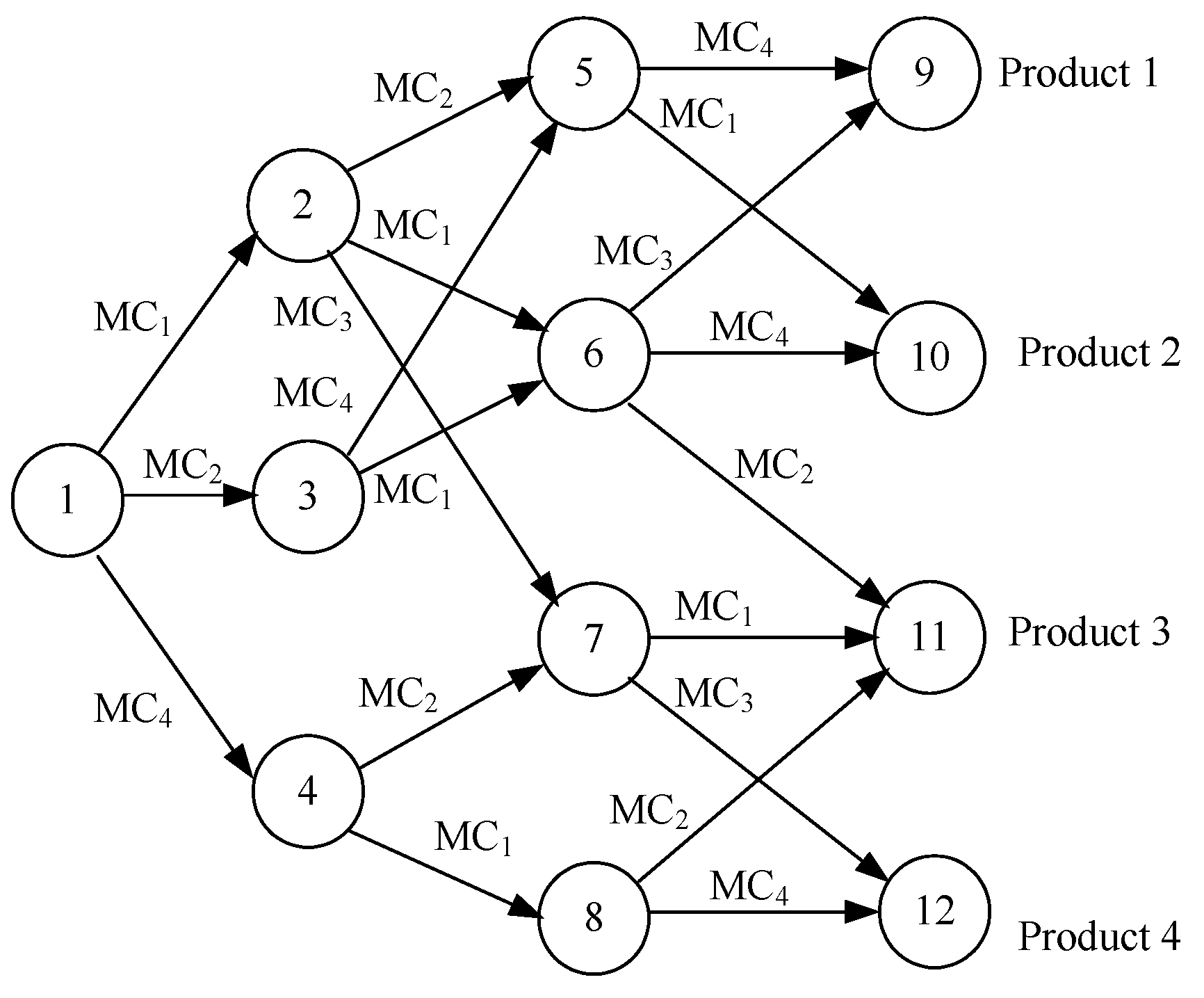
Two test examples were provided by Anjie Guo [26]. The first one is a small problem with three products and six nodes, as shown in Figure 3. The second one is a large problem with four products and 12 nodes, as shown in Figure 5. In both problems, the interarrival times of orders follow a normal distribution with a mean of 30 and a standard deviation of 5. The risk is α = 10%. The computational experiment was coded in MATLAB 9.1 (R2016b) (MathWorks: Natick, MA, USA) and conducted using an Intel Core i7, 3.2 GHz CPU, 4 GB RAM computer.
In the small problem, each order has a batch of 10, and the probabilities for Products 1, 2, and 3 are 0.5, 0.35, and 0.15, respectively. The time horizon H is 600, so 200 sets of raw material are ordered. The processing times for 1-2, 1-3, 2-4, 2-5, 3-5, and 3-6 are normally distributed with parameters (4,1), (3,1), (5,2), (4,1), (4,1) and (3,1). In the large problem, each order has a batch of 10, and the probabilities for Products 1, 2, 3, and 4 are 0.5, 0.25, 0.1, and 0.15, respectively. The time horizon H is 1200, so 400 sets of raw material are ordered. The processing times for 1-2, 1-3, 1-4, 2-5, 2-6, 2-7, 3-5, 3-6, 4-7, 4-8, 5-9, 5-10, 6-9, 6-10, 6-11, 7-11, 7-12, 8-11 and 8-12 are normally distributed with parameters (4,1), (3,1), (5,2), (4,1), (4,1), (5,2), (4,2), (4,1), (5,1), (4,2), (3,1), (5,2), (5,1), (4,1), (5,1), (3,1), (4,2), (5,2) and (4,1).
In the two problems, the RMTS was trained off-line by arbitrarily selecting M = 9604 x from the search space, and their F s ( x ) was estimate by precise evaluation. The sampling value M = 9604 was calculated by the sample size formula using a confidence level of 95% and a confidence interval of 1% [27]. In the choice of parameters for modeling RMTS, σ = 0.5 and ρ = 10 14 were obtained by the analytic approach.
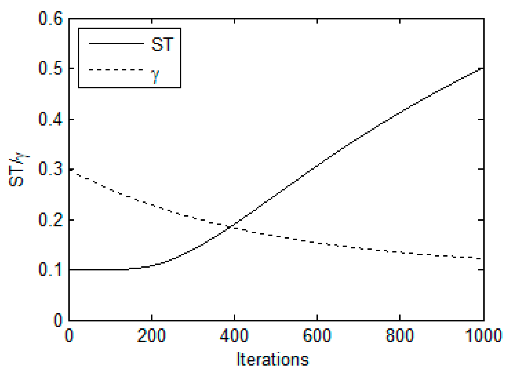
For the small problem, the penalty weight λ was 0.9. The number of outstanding solutions was N = 5. The parameters used in Algorithm 1 were obtained by a series of hand-tuning experiments as: Ψ = 10, S T min = 0.1 , S T max = 0.5 , γ min = 0.1 , γ max = 0.3 , and k max = 1000 . Elementary experiments demonstrated that ITSA with these parameters performed uniformly better over 30 independent runs. The developed ITSA favorably explored the entire search space at the early iterations and likely exploited excellent solutions at the later iterations. As the search evolved, the values of ST and γ were dynamically changed to strengthen diversification at first and intensification toward the end. Figure 6 presents the trends of ST and γ over iterations. The value of ST is exponentially increased. A small value of ST favors diversity in the beginning, while a large value makes fine tuning ability near the end. The parameter γ exponentially decreased to achieve the balance between exploration and exploitation. At the beginning, most of the search utilized randomly selected pitches to accomplish global exploration. As the searching process progressed, γ was exponentially decreased and the search progressively revolved around the best tree in memory to realize local exploitation.
The parameters of Algorithm 2 were L 0 = 20, Δ = 10 and L s = 10 4 . The reduction factor s corresponded to N = 5 is 2.08 [22]. Thus, the available computing budget C b was 24038. Table 1 shows the excellent solution x , the corresponding E [ f ( x ) ] , P ( g ( x ) b ) , F ( x ) and the consumed CPU times.
For the large problem, the penalty weight λ was also 0.9. The parameters in Algorithm 1 were: Ψ = 50, S T min = 0.1 , S T max = 0.5 , γ min = 0.1 , γ max = 0.3 , and k max = 2000 . The parameters in Algorithm 2 were: L 0 = 20, Δ = 10 and L s = 10 4 . To find the relationship between the computing effort and solution quality, four values of N were simulated in Algorithm 2: N = 20, 15, 10 and 5. The reduction factors corresponding to N = 20, 15, 10 and 5 were s = 6.07, 4.72, 3.4 and 2.08 [22], respectively. Thus, the available computing budgets were C b = 32949, 31780, 29412 and 24038 for N = 20, 15, 10 and 5, respectively. Table 2 lists the excellent solution x , the corresponding E [ f ( x ) ] , P ( g ( x ) b ) , F ( x ) and the CPU times. When the value of N increases, the corresponding E [ f ( x ) ] decreases but the CPU time increases. In principle, the value of N depends on the available computing budget for various applications. From the results shown in Table 2, N = 20 is a suggested choice for the large problem. The CPU times in all cases were less than 100 s, which is short enough for real-time purposes. Besides, the inter-arrival times of orders and processing times of tasks can exhibit any distribution, and the dimensions of the problem can be high.
There is no systematic procedure to obtain the preferable and robust values of the following control parameters, [ S T min , S T max ] , [ γ min , γ max ] and N . Although a proper parameter setting can help to have a good performance, such setting is very problem dependent. After analyzing the influence on convergence rate and solution accuracy, the preferable values of [ S T min , S T max ] , [ γ min , γ max ] and N were obtained by a series of hand-tuning experiments for the considered problem.

4.2. Comparisons of Large Problem

To illustrate the computing efficiency of the proposed method, three heuristic methods, PSO, GA and ES, were used to solve the large problem with precise evaluation. The parameters used in the PSO [28] were: both social factor and cognitive factor were 2; the maximum permissible velocity was 0.5; inertia factor was 1; and size of population was 50. The parameters used in the GA [29] were: size of population was 50; crossover rate was 0.8; and mutation rate was 0.03. A real-value coding, single point crossover and roulette wheel selection were employed in the GA. The parameters used in the ES [30] were: size of population was 50, number of offspring was 100, and mutation strength constant was 1 / 12 . It should be noted that the precise evaluation was used to estimate the objective value for each method.
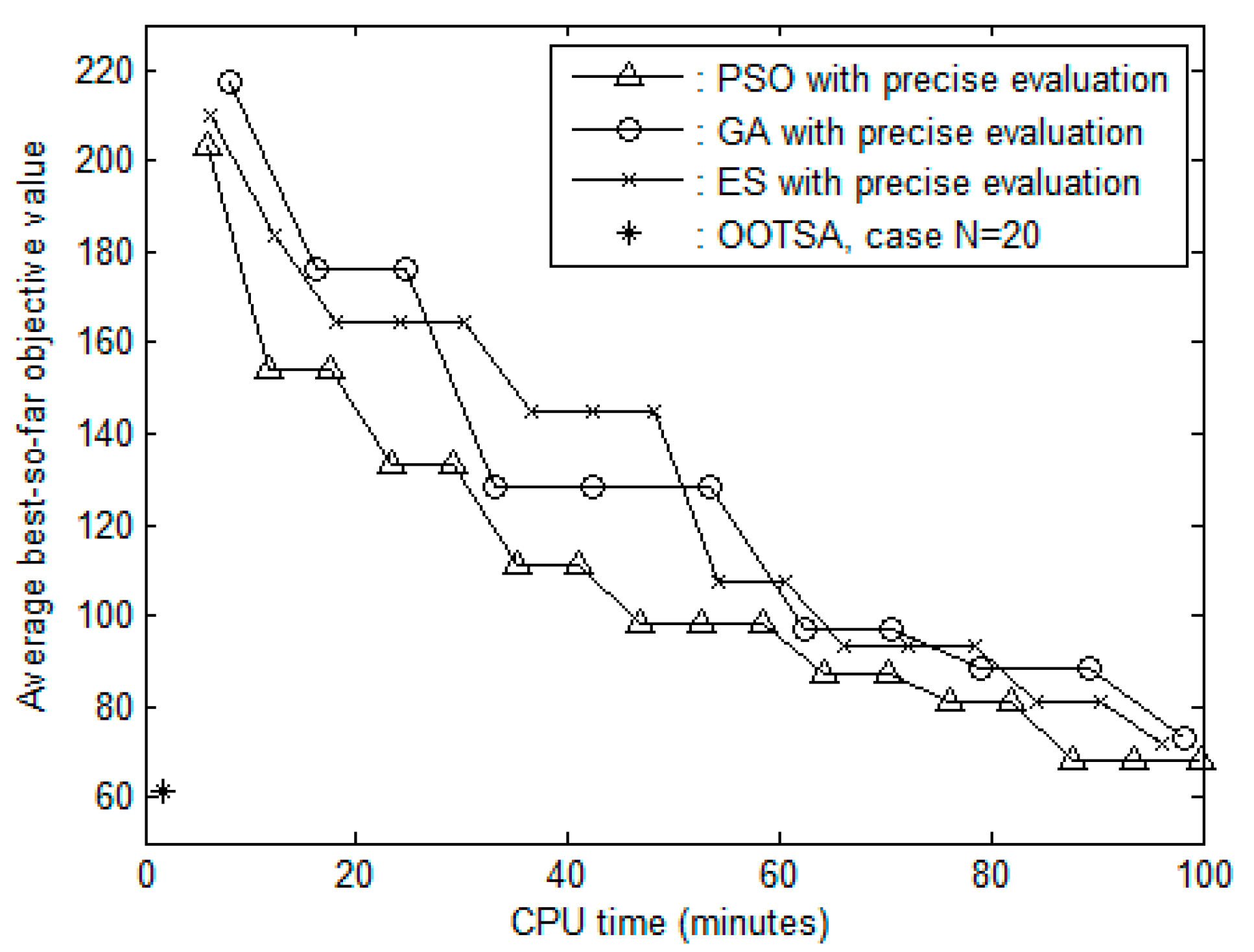
The large problem was simulated over 30 independent runs. Because the three heuristic methods spend a long period obtaining the optimal solutions, we terminated their executions when they had spent 100 min of CPU time. Since the case N = 20 takes the longest consumed CPU time in large problem, progression result obtained using the OOTSA for case N = 20 was compared with three heuristic methods. Figure 7 shows the solution qualities and computational efficiencies obtained by four methods for 30 independent runs. The “ ” point with coordinates (1.61, 61.55) shown in Figure 7 represents the pair of (consumed CPU time, average obtained objective value F ( x ) ) obtained using the OOTSA for case N = 20. The progressions of the average best-so-far objective value and the corresponding consumed CPU times at the end of every iteration of three competing methods are also shown in Figure 7. The progressions of these values associated with PSO, GA and ES are plotted as solid lines with triangles “ Applsci 08 02153 i001”, solid line with open circles “ Applsci 08 02153 i002”, and solid line with crosses “ Applsci 08 02153 i003”, respectively. Table 3 demonstrates that the average best-so-far objective values that were obtained by PSO, GA and ES were 10.74%, 18.47% and 16.21% larger than that obtained by OOTSA. The average best-so-far objective values obtained by the three heuristic methods were worse than not only that determined by the OOTSA with N = 20, but also those obtained using the three other values of N . Test results reveal that the OOTSA approach frequently determines an excellent solution in a limited amount of time and significantly outperforms three heuristic methods with precise evaluation.
Subsequently, the solution quality of the OOTSA is appreciable. To judge the global optimality of the obtained solution, the rankings of the solution resulted from four methods were compared. It is impossible to compare the rankings of all solutions in the entire search space. Accordingly, a representative subset, Θ , was constructed to substitute the large search space. We arbitrarily selected 16,641 solutions from search space to construct the representative subset Θ and utilizes the precise evaluation to estimate their objective values. The size | Θ | = 16,641 was calculated by the sample size formula using a confidence level of 99% and a confidence interval of 1% [27].
A ranking rate analysis was performed to represent the ranking of a solution in the representative subset Θ . The ranking rate is defined as r k / | Θ | × 100 % , where r k is the ranking of a solution, which can easily be determined from its objective value. Table 4 lists statistics of the objective value and average ranking rate over 30 independent runs that were obtained by four approaches. The mean, standard deviation and standard error of mean of the objective value obtained by the OOTSA for N = 20 over 30 independent runs were 61.55, 0.52 and 0.0949, respectively. The tiny standard error of mean reveals that most of the objective value obtained by the OOTSA is around the mean or practically near the best solution over 30 independent runs. Thus, the OOTSA approach can usually determine an excellent solution, even if it is not a global optimal solution.

5. Conclusions

To resolve the computationally expensive PCSOP for an excellent solution in a reasonable amount of time, a method that embeds OO into TSA is presented. The developed method has three modules: surrogate model, exploration and exploitation. The RMTS surrogate model approximated a solution quickly. The developed method integrated the ITSA for exploration with the IOCBA for exploitation. The ITSA achieved the diversification at first and shifted toward intensification of good solutions near the end. The IOCBA improved the efficiency of simulation to determine an excellent solution. The proposed method was employed to a pull-type production system, which is formulated as a PCSOP. The proposed method was compared with three heuristic methods, PSO, GA and ES, with precise evaluation. The excellent solution obtained by the proposed method provided a high solution quality with beneficial computing efficiency. Simulation results reveal that most objective values obtained by the OOTSA are around the mean or practically near the best solution in several runs. The proposed method can frequently determine an excellent solution even if it is not a global optimal solution. Actually, the proposed OOTSA approach can be applied to solve most industrial optimization problems, such as picking strategy in food supply chain [31], ergonomic assessment in infrequent job rotations [32], production–distribution planning in supply chain systems [33], dynamic job shop scheduling problems [34], and minimal cost of supply chain management [35]. Further research will address extension of the proposed method to consider more complex probabilistic constrained model, such as perishable inventory management problem and portfolio financial optimization problem.

Author Contributions

S.-C.H. conceived and designed the experiments; S.-C.H. performed the experiments; S.-S.L. analyzed the data; S.-S.L. contributed reagents/materials/analysis tools; and S.-C.H. wrote the paper.

Funding

This research work was supported in part by the Ministry of Science and Technology in Taiwan, under Grant MOST107-2221-E-324-021.

Conflicts of Interest

The authors declare no conflict of interest.

References

  1. Ghanem, R.; Soize, C. Probabilistic nonconvex constrained optimization with fixed number of function evaluations. Int. J. Numer. Methods Eng. 2018, 113, 719–741. [Google Scholar] [CrossRef]
  2. Lejeune, M.A.; Shen, S.Q. Multi-objective probabilistically constrained programs with variable risk: Models for multi-portfolio financial optimization. Eur. J. Oper. Res. 2016, 252, 522–539. [Google Scholar] [CrossRef]
  3. Chen, J.F.; Nair, V.; Menzies, T. Beyond evolutionary algorithms for search-based software engineering. Inf. Softw. Technol. 2018, 95, 281–294. [Google Scholar] [CrossRef] [Green Version]
  4. Chang, M.X.; Chang, W.Y. Efficient detection for MIMO systems based on gradient search. IEEE Trans. Veh. Technol. 2016, 65, 10057–10063. [Google Scholar] [CrossRef]
  5. Triki, C.; Mirmohammadsadeghi, S.; Piya, S. Heuristic methods for the periodic shipper lane selection problem in transportation auctions. Comput. Ind. Eng. 2017, 106, 182–191. [Google Scholar] [CrossRef]
  6. Ertenlice, O.; Kalayci, C.B. A survey of swarm intelligence for portfolio optimization: Algorithms and applications. Swarm Evolut. Comput. 2018, 39, 36–52. [Google Scholar] [CrossRef]
  7. Mavrovouniotis, M.; Li, C.H.; Yang, S.X. A survey of swarm intelligence for dynamic optimization: Algorithms and applications. Swarm Evolut. Comput. 2017, 33, 1–17. [Google Scholar] [CrossRef] [Green Version]
  8. Piotrowski, A.P.; Napiorkowski, M.J.; Napiorkowski, J.J.; Rowinski, P.M. Swarm intelligence and evolutionary algorithms: Performance versus speed. Inf. Sci. 2017, 384, 34–85. [Google Scholar] [CrossRef]
  9. Ho, Y.C.; Zhao, Q.C.; Jia, Q.S. Ordinal Optimization: Soft Optimization for Hard Problems; Springer: New York, NY, USA, 2007. [Google Scholar]
  10. Horng, S.C.; Lin, S.S. Embedding advanced harmony search in ordinal optimization to maximize throughput rate of flow line. Arab. J. Sci. Eng. 2018, 43, 1015–1031. [Google Scholar] [CrossRef]
  11. Horng, S.C.; Lin, S.S. Ordinal optimization based metaheuristic algorithm for optimal inventory policy of assemble-to-order systems. Appl. Math. Modell. 2017, 42, 43–57. [Google Scholar] [CrossRef]
  12. Horng, S.C.; Lin, S.S. Merging crow search into ordinal optimization for solving equality constrained simulation optimization problems. J. Comput. Sci. 2017, 23, 44–57. [Google Scholar] [CrossRef]
  13. El-Fergany, A.A.; Hasanien, H.M. Tree-seed algorithm for solving optimal power flow problem in large-scale power systems incorporating validations and comparisons. Appl. Soft Comput. 2018, 64, 307–316. [Google Scholar] [CrossRef]
  14. Babalik, A.; Cinar, A.C.; Kiran, M.S. A modification of tree-seed algorithm using Deb’s rules for constrained optimization. Appl. Soft Comput. 2018, 63, 289–305. [Google Scholar] [CrossRef]
  15. Cinar, A.C.; Kiran, M.S. Similarity and logic gate-based tree-seed algorithms for binary optimization. Comput. Ind. Eng. 2018, 115, 631–646. [Google Scholar] [CrossRef]
  16. Kiran, M.S. TSA: Tree-seed algorithm for continuous optimization. Expert Syst. Appl. 2015, 42, 6686–6698. [Google Scholar] [CrossRef]
  17. Hwang, J.T.; Martins, J.R.R.A. A fast-prediction surrogate model for large datasets. Aerosp. Sci. Technol. 2018, 75, 74–87. [Google Scholar] [CrossRef]
  18. Igarashi, Y.; Yabe, H. A primal-dual exterior point method with a primal-dual quadratic penalty function for nonlinear optimization. Pac. J. Optim. 2015, 11, 721–736. [Google Scholar]
  19. Smith, R.C. Uncertainty Quantification: Theory, Implementation, and Applications; SIAM: Philadelphia, PA, USA, 2014. [Google Scholar]
  20. Niutta, C.B.; Wehrle, E.J.; Duddeck, F.; Belingardi, G. Surrogate modeling in design optimization of structures with discontinuous responses. Struct. Multi. Optim. 2018, 57, 1857–1869. [Google Scholar] [CrossRef]
  21. Kang, L.L.; Joseph, V.R. Kernel approximation: From regression to interpolation. SIAM-ASA J. Uncertain Quantif. 2016, 4, 112–129. [Google Scholar] [CrossRef]
  22. Chen, C.H.; Lee, L.H. Stochastic Simulation Optimization: An Optimal Computing Budget Allocation; World Scientific: New Jersey, NJ, USA, 2010. [Google Scholar]
  23. Karakul, P.M.; Dasci, A. An approximation method to analyse polling models of pull-type production systems. Eur. J. Ind. Eng. 2007, 1, 200–222. [Google Scholar] [CrossRef]
  24. Ulewicz, R.; Nowakowska-Grunt, J.; Jelonek, D. Performance evaluation of the production control systems of push and pull type. Appl. Mech. Mater. 2015, 795, 235–242. [Google Scholar] [CrossRef]
  25. Tseng, T.; Gung, R.R.; Huang, C. Performance evaluation for pull-type supply chains using an agent-based approach. Am. J. Ind. Bus. Manag. 2013, 3, 91–100. [Google Scholar] [CrossRef]
  26. SimOpt.org. Strategic Location of Semi-Finished Products. Available online: http://simopt.org/wiki/index.php?title=Strategic_Location_of_Semi-Finished_Prod, 2016 (accessed on 16 June 2016).
  27. Ryan, T.P. Sample Size Determination and Power; John Wiley and Sons: Hoboken, NJ, USA, 2013. [Google Scholar]
  28. Qian, W.Y.; Li, M. Convergence analysis of standard particle swarm optimization algorithm and its improvement. Soft Comput. 2018, 22, 4047–4070. [Google Scholar] [CrossRef]
  29. Pathan, M.V.; Patsias, S.; Tagarielli, V.L. A real-coded genetic algorithm for optimizing the damping response of composite laminates. Comput. Struct. 2018, 198, 51–60. [Google Scholar] [CrossRef]
  30. Abad, A.; Elipe, A. Evolution strategies for computing periodic orbits. Math. Comput. Simul. 2018, 146, 251–261. [Google Scholar] [CrossRef]
  31. Facchini, F.; De Pascale, G.; Faccilongo, N. Pallet picking strategy in food collecting center. Appl. Sci. 2018, 8, 1503. [Google Scholar] [CrossRef]
  32. Boenzi, F.; Facchini, F.; Digiesi, S.; Mummolo, G. Ergonomic improvement through job rotations in repetitive manual tasks in case of limited specialization and differentiated ergonomic requirements. IFAC-PapersOnLine 2016, 49, 1667–1672. [Google Scholar] [CrossRef]
  33. Sakalli, U.S.; Atabas, I. Ant colony optimization and genetic algorithm for fuzzy stochastic production-distribution planning. Appl. Sci. 2018, 8, 2042. [Google Scholar] [CrossRef]
  34. Park, J.; Mei, Y.; Nguyen, S.; Chen, G.; Zhang, M.J. An investigation of ensemble combination schemes for genetic programming based hyper-heuristic approaches to dynamic job shop scheduling. Appl. Soft Comput. 2018, 63, 72–86. [Google Scholar] [CrossRef]
  35. Yao, B.Z.; Chen, G. Stochastic simulation and optimization in supply chain management. Simulation 2018, 94, 561–562. [Google Scholar] [CrossRef] [Green Version]
Figure 1. Structure of a regularized minimal-energy tensor-product splines.
Applsci 08 02153 g001
Figure 2. Flow chart of the proposed OOTSA approach.
Applsci 08 02153 g002
Figure 3. Three product pull-type production system.
Applsci 08 02153 g003
Figure 4. The input–output relationship in pull-type production system.
Applsci 08 02153 g004
Figure 5. Four product production system.
Applsci 08 02153 g005
Figure 6. Variations of ST and γ over iterations.
Applsci 08 02153 g006
Figure 7. Comparison of the computing efficiency and solution quality of four methods over 30 independent runs.
Applsci 08 02153 g007
Table 1. The excellent solution x , the corresponding E [ f ( x ) ] , P ( g ( x ) b ) , F ( x ) and the consumed CPU times of small problem.
x   E [ f ( x ) ]   P ( g ( x ) b )   F ( x )   CPU Times (s)
[19,28,28,42,42,41]T10.720.90099.64824.67
Table 2. The excellent solution x , the corresponding E [ f ( x ) ] , P ( g ( x ) b ) , F ( x ) and the consumed CPU times for four values of N in large problem.
N x   E [ f ( x ) ]   P ( g ( x ) b )   F ( x )   CPU Times (s)
20[51,49,48,47,48,30,29,20,20,20,19,19]T68.390.900261.5696.35
15[52,47,48,49,49,29,29,20,20,19,19,19]T69.750.901362.7793.41
10[53,48,49,48,47,29,30,20,20,19,19,18]T70.940.902463.8490.94
5[54,49,47,48,48,30,29,20,19,18,20,18]T71.390.901964.2589.17
Table 3. Statistics of the average best-so-far objective values at termination over 30 independent runs.
MethodsABOV ABOV § · 100 %
OOTSA, case N = 2061.550
PSO with precise evaluation68.1610.74%
GA with precise evaluation72.9218.47%
ES with precise evaluation71.5316.21%
ABOV, average best-so-far objective value F ( x ) at termination. § *, average best-so-far objective value obtained by OOTSA.
Table 4. Statistics of the objective values and average ranking rate over 30 independent runs.
ApproachesMinimumMaximumMeanStandard DeviationStandard Error of the MeanAverage Ranking Ate
OOTSA, case N = 2060.3762.9761.550.520.09490.002%
PSO with precise evaluation66.5670.4268.160.760.13880.562%
GA with precise evaluation70.3875.8172.921.030.18810.821%
ES with precise evaluation69.9173.6871.530.870.15880.658%