1. Introduction
Two-fluid flow in a porous medium is an application of importance in many fields of science including petroleum engineering, environmental engineering, hydrology, and soil science. In addition, organismic systems are sometimes considered to be porous media [
1,
2,
3]. Mathematical models are routinely used in each of these fields to describe fluid flow, make predictions, and guide designs. The traditional model used to describe two-fluid flow was first formulated nearly a century ago [
4], although this formulation was for the simplified case that is often attributed to Richards [
5]. The extension of this model to the two fluid case for which pressures are resolved in both phases is straightforward. The conservation of mass equations alone do not lead to a closed model, so closure relations are needed to produce a solvable system. These closure relations traditionally include a relationship between fluid pressures and fluid saturations, a relationship between fluid saturations and relative permeabilities for each fluid phase, and equations of state if the fluid densities change with respect to pressure; we will neglect species or thermal transport. Collectively, we will refer to this as the traditional model and details are available in the literature [
6]. Thousands of papers have been written on various aspects of the traditional model for two-fluid flow through a porous medium systems, including forms of the closure relations [
7,
8], mathematical analysis of the solution characteristics [
9,
10], numerical approximation methods intended to approximate the resultant model [
11,
12,
13], computational science algorithms intended to produce efficient solution methods [
14], and application to many different systems [
15,
16]. Much less work has been accomplished to advance the theory of two-fluid-phase flow, although significant shortcomings exist with the traditional approach.
The traditional model for two-fluid-phase flow in porous media is formulated phenomenologically at the macroscale where a point represents averaged conditions over a region that includes all phases. The microscale, or pore-scale, is an alternative scale where the locations of juxtaposed phases are resolved in space and in time. At the microscale, the importance of interfacial areas, common curve lengths, contact angles, interfacial and curvilinear tensions and curvatures, and phase orientations are understood to be important. However, none of these noted microscale quantities enter the traditional macroscale model explicitly. Furthermore, common pressure-saturation relations are nonlinear, hysteretic, and apply only to equilibrium conditions [
17,
18]. These relations also include further empirical representations for the entrapped non-wetting phase and a quantity known as the irreducible wetting-phase saturation, which can be misnomer because wetting-phase saturations below the irreducible level routinely occur as a result of a mass transfer process from the wetting phase to the non-wetting phase (e.g., evaporation, dissolution). Common relative permeability relations are hysteretic relations that depend upon the fluid saturation history and are empirical in nature [
6,
19,
20,
21]. Limitations of the traditional model also include the lack of a precise connection between microscale quantities and macroscale quantities, because the macroscale model is formulated phenomenologically and does not emerge from a formal upscaling procedure. It has also been shown that although the traditional model assumes an equilibrium state between saturation and the fluid-fluid pressure difference that this condition is unlikely to exist for most systems [
22], though some models have been developed that do not rely upon this assumption [
23,
24]. Despite these several limitations, resolving these issues has not received much attention in the literature.
The overall goal of this work is to report advances to a new generation of two-fluid-flow models that responds to the limitations associated with traditional approaches. Alternatives to this new generation of models exist and are reviewed elsewhere [
25,
26,
27]. The specific objectives of this work are: (1) to summarize the previously developed thermodynamically constrained averaging theory (TCAT) approach for building models that are both scale and thermodynamically consistent; (2) to summarize the application of the TCAT procedure for two-fluid flow; (3) to examine an example instance of a TCAT model for two-fluid flow; (4) to demonstrate how hysteresis can be removed using a state equation involving capillary pressure and how the parameters for this state equation can be determined; (5) to explore the existence of a state equation to approximate the conservation of momentum at the macroscale; and (6) to summarize the challenges that must be overcome to complete the formulation of this new class of two-fluid flow model.
2. Thermodynamically Constrained Averaging Theory
A wide range of length scales exist and the terminology used to describe these length scales varies in the literature. For our purposes, three discrete length scales are of concern to support the discussion that follows. The microscale is a length scale that is long compared to the mean distance between molecular collisions or the vibrational scale for a solid. At the microscale a point represents an averaging region that is related to the lower bound on the length scale needed for the laws of continuum mechanics to apply. Another characteristic of the microscale is that a point exists entirely within an individual phase, even in a system that includes multiphase phases (fluids, solids). Porous medium systems are systems that contain multiple phases by definition. At the microscale, the morphology and topology of the phase distributions are resolved in time. For porous medium systems, the microscale is oftentimes referred to as the pore scale.
The second scale of concern herein is the macroscale. The macroscale is a scale where phase distributions are resolved only in an averaged sense; a point is the centroid of an averaging region which extends over all phases, interfaces, common curves, and common points that exist in a system. Macroscale extent measures involve concepts such as volume fractions, fluid saturations, specific interfacial areas, and specific common curve lengths. The boundaries of the phases are not resolved at the macroscale, only the averaged extent measures are resolved. Macroscale representations are necessary to make many systems of interest tractable, including engineered systems such as filters and reactors and natural systems such as subsurface porous medium systems, including petroleum reservoirs. This is so because even for cases in which microscale details of phase distribution are accessible, computational limitations of even the world’s fastest computers precludes the detailed simulations of systems at the scale of applications of concern, say the unsaturated zone above an aquifer. Macroscale representations are also used as a simplification when microscale details are unnecessary for the problem of interest.
The third scale of interest is termed the megascale, and it is the overall length scale of the system of concern, which might vary greatly in size between a model laboratory system, an engineered system, and a natural system. What is common at the megascale however is that the details of the spatial distribution of quantities within the system are not resolved. Instead, inputs and outputs from the system are considered only on the boundaries of the system. Oftentimes systems may be considered megascale in one or two dimensions and say macroscale in the remaining dimensions. An example of such an instance is the treatment of a subsurface region in a vertically averaged fashion [
28,
29,
30]; only spatial variations in the horizontal plane are resolved.
The typical situation is that macroscale models are phenomenological in nature—meaning conservation equations are written following an assumed form usually based upon a presumed extension of microscale principles, which are better understood. Then the macroscale models are typically closed using empirical relations intended to represent small-scale behavior in a simplified, yet meaningful and tractable manner. The literature is replete with such examples, and flow and transport phenomena in porous medium systems is a prime class of example [
31]. The phenomenological approach can lead to solvable systems that enable solutions, but the general procedure is fraught with problems, many of which are not well understood because the general approach is deeply ingrained in text books [
32,
33,
34] and practice, and generally accepted.
The phenomenological approach of model formulation suffers from several problems [
25,
35]. First, fundamental microscale physics may not be naturally and explicitly present in posited macroscale models. Second, certain microscale principles, such as thermodynamics, are often completely ignored. Third, quantities that appear in macroscale models may not be precisely defined in terms of microscale quantities, precluding a rigorous connection between microscale systems and macroscale systems. Fourth, macroscale closure relations are often constructs of convenience intended to produce solvable systems but not deduced from fundamentals or constrained to obey thermodynamic principles, such as the second law of thermodynamics. Fifth, phenomenological models are typically evaluated and validated by comparing to the overall system of concern, and when they fail to provide an adequate description a new model must be formulated without a rigorous, well-defined procedure to do so. TCAT has been developed to resolve these issues associated with standard phenomenological approaches [
25,
35,
36,
37].
TCAT is an approach for building classes, or hierarchies, of models of varying sophistication and fidelity, which can be matched to the needs of a given application. The problems noted above with the phenomenological approach are overcome with the TCAT approach.
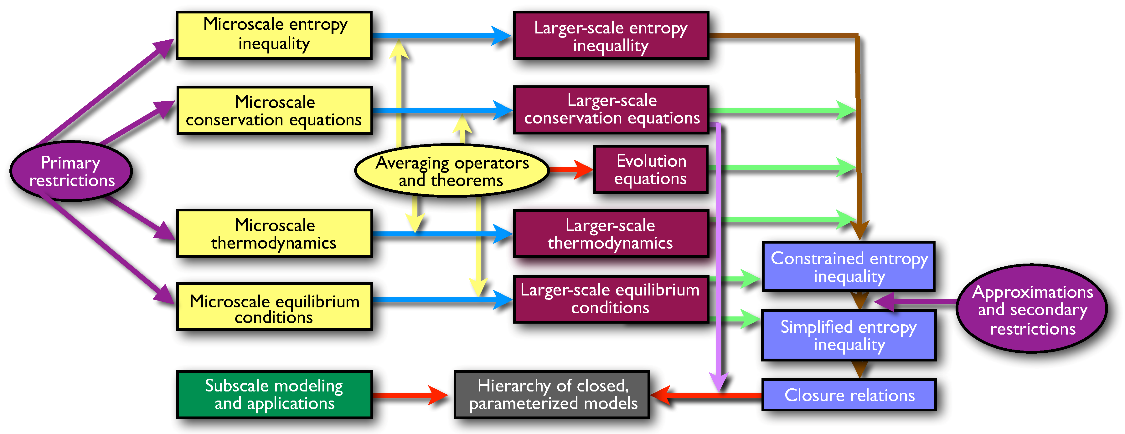
Figure 1 is a graphical depiction of the TCAT approach. The general flow is left to right, then top to bottom, with the final desired result appearing in the gray box in middle of the bottom of this schematic diagram. Substantial mathematical details, using a variety of methods, are involved in the overall approach and component parts that have been derived [
35,
36]. Rather than focus on these mathematical details, we will consider the conceptual approach, the inter-relationship of the component parts shown, and explain some attributes of the approach that respond to weaknesses in phenomenological approaches.
Primary restrictions form a basic set of statements needed to frame and define a hierarchy of models of concern. The way in which this is done is a balance between the degree of generality sought in the model framework formulated at a larger scale, which denotes some scale(s) above the microscale. Aspects of the primary restrictions affecting this generality include the entities of concern and the nature of the phenomena one intends to model. Entities refer to phases, interfaces, common curves, and common points. Phenomena being modeled is some combination of mass, momentum, and energy in entities or species within entities. Primary restrictions are also needed to specify a microscale thermodynamic theory that will be relied upon and certain requirements on the separation of length scales [
36].
Primary restrictions can be stated such that only one specific model is sought [
37]. The advantage to this approach is simplicity in the model formulation process. The disadvantage is that the formulation has a limited opportunity to be reused and adapted for other models of concern. On the opposite end of the generality scale, one could formulate a model framework for an arbitrary number of entities, species transport of all quantities, and a general reference velocity. While such an approach would have applicability to a wide class of problems, the generality would impede the development of specific models. The approach taken to date is to seek a middle ground where general hierarchies of models of a given class are formulated by specifying the set of entities and what combination of entity-species transport is to be considered. This approach results in a given TCAT formulation for a class of models that has many possible instances, thus supporting reuse. This is important because the model formulation process is technical, but many of these details can be neglected in the generation of specific models from a general hierarchy—allowing relatively straightforward reuse and broad applicability.
The yellow rectangles in
Figure 1 represent fundamental components in the model-building process. Microscale conservation equations for phases are well established in the continuum mechanics and transport phenomena literature [
38], but the equations needed for lower-dimensional entities are rarely considered [
36]. A microscale thermodynamic theory must be chosen for TCAT, and we have relied upon classical irreversible thermodynamics to date due to the utility of the TCAT results produced relying upon this theory. It is also necessary to determine conditions that must hold at equilibrium for systems consisting of sets of entities, which is a topic that is not standard in most thermodynamics references. Together, these components form the microscale fundamentals needed to generate larger scale models.
The blue arrows in
Figure 1 represent the integration of microscale equations over a representative elementary region, normalization by the volume of the averaging region, and simplification to a convenient form. Averaging operators and averaging theorems enable the accomplishment of these manipulations [
35,
36,
39,
40,
41]. The maroon rectangles represent the result of these manipulations. Evolution equations are derived based upon averaging theorems alone, as well as the application of some approximations needed to arrive at convenient forms. Evolution equations aid in the formulation of closed models by supplying equations that supplement the conservation equations and reduce the deficit between the number of unknowns in a model and the number of available equations, which is the closure problem that occurs in mechanistic modeling.
The closure problem is solved in TCAT by formulating an expression for the entropy density production rate, which is known to be non-negative by the second law of thermodynamics. To express the entropy density production rate in terms of dissipative processes that can produce entropy, the conservation and thermodynamic equations are introduced in a form that does not change the inequality. The result of what is a detailed calculation for a given class of problems is the constrained entropy inequality (CEI), which is an essentially exact equation. The CEI, while exact, is not in the desired flux-force form. To derive such a form, approximations are needed, which when applied yield a simplified entropy inequality (SEI) in strict flux-force form. The SEI is a statement of the second law of thermodynamics that connects the dissipative processes with the rate of entropy production—allowing for consistent approximations to be posited for a set of closure relations that along with the conservation and evolution equations form a closed, solvable model. Multiple sets of closure relations may be specified that are consistent with the SEI, so the SEI can be considered as a set of permissibility conditions for model closure. The result of this procedure is a specific closed model. Different secondary restrictions or alternative sets of closure relations yield different models. Thus, the TCAT procedure as typically implemented is said to yield a hierarchy of closed models of varying sophistication and fidelity.
Because the larger scale TCAT models are derived from a formally defined upscaling of microscale principles, microscale experimental observations or simulations can be averaged in this same specific manner and used to evaluate and validate TCAT models [
22,
36]. Microscale simulations, or experiments, can also be used to determine parameters needed in closure relations appearing in a TCAT model.
TCAT model hierarchies have been derived for single- and two-fluid flow [
42,
43], single- and two-fluid species and heat transport [
40,
44,
45,
46], single-fluid megascale flow [
47], the transition between a porous medium system and a single fluid system [
48], and recently for sediment transport in surface water systems [
49]. While much of the theory work has been accomplished for a wide range of applications, relatively few model cases have been examined in detail, solved, evaluated and validated [
50]. This is one of the disadvantages of theoretical work of this sort—several steps taken for granted in traditional modeling approaches, including formulation of the closure relation forms, determination of model parameters, numerical approximation of the resultant model form, and model evaluation and validation, must be carefully repeated because many aspects of the model formulation change when one is using the TCAT approach. In the sections that follow we examine the specific case of two-fluid flow through a porous medium system, considering not only the formulation and an example model form but also the evaluation and validation of certain aspects of the model.
3. Model Formulation
The TCAT approach has been applied to derive a hierarchy of models for two-fluid-phase flow in a porous media [
22,
27,
36,
43]. The approach taken will be summarized and compared to the traditional approach, and a specific model instance from the general hierarchy of models available will be formulated to focus on the novel aspects of this work.
Traditional models are based on a conservation of mass equation and an extension of Darcy’s law to approximate the conservation of momentum for the fluid phases, and these model components are formulated directly at the macroscale. The TCAT approach starts from conservation of mass, momentum, and energy equations, and a balance of entropy for all three phases, the three interfaces that can form between pairs of phases, and the common curve where all three phases intersect; all of these equations are formulated at the microscale, along with thermodynamic equations. The set of microscale equations are averaged to the macroscale, providing a direct connection between microscale quantities and macroscale quantities. The inclusion of interfaces and common curves is a key aspect of the approach and provides a basis for the important microscale physics (interfacial areas, contact angles, interfacial tension, curvatures, etc.) to emerge in the macroscale models. The macroscale equations are then used to derive a general SEI [
36], which is in turn used to formulate closure relations that are assured to be consistent with the second law of thermodynamics.
The TCAT approach described above is general and can support a wide range of models, including non-isothermal systems, complex solid behavior, a full range of entities (phases, interfaces, and common curves), and the exchange of all quantities among the entities. Alternatively, the general formulation can be restricted to any case that is a subset of the general formulation, specific evolution equations can be added to the formulation, and the remaining closure problem can be considered. Resolving the closure problem in a rigorous fashion is an important aspect of the TCAT model development process.
We will focus on a specific restricted form of a two-fluid-phase flow model that is sufficiently complex to reveal several interesting aspects of the approach and to pose a set of challenges that must be overcome to formulate a complete closed and solvable model. Specifically, we consider the restricted case in which the porosity is constant, the system is isothermal, interfaces are massless, mass transfer between entities does not occur, and common curves are neglected. The resultant model consists of two conservation of mass equations for the fluid phases
and a momentum equation for each fluid phase
where
is the volume fraction,
is the mass density,
t is time,
is the velocity vector,
is the index set of fluid phases,
is an entity qualifier,
is a fluid pressure,
is gravitational acceleration vector, the subscript and superscript
w denotes the wetting phase and
n the non-wetting phase, and
,
, and
are resistance coefficients. The adornments on the superscripts denote the particular types of averages [
36] with an unadorned symbol denoting a volume average, a single overbar symbol a density weighted average, and a double-overbar symbol a specially defined average. The hatted symbols denote material parameters.
In addition to conservation equations, evolution equations provide additional sources of information to formulate mechanistic models. Evolution equations are equations based on averaging theorems, rather than conservation principles, and express relationships among geometric quantities. An evolution equation for the wetting-phase volume fraction is
and an evolution equation for the fluid-fluid interfacial area is
where
is a coefficient related to the relaxation of the interfacial area to an equilibrium state,
is the specific interfacial area,
is the interfacial tension between the fluid phases,
is the specific interfacial area of the
interface at equilibrium,
is a coefficient related to the rate of relaxation of the capillary pressure to an equilibrium state,
is the capillary pressure,
is twice the mean curvature of the fluid-fluid interface, and
is the fluid-fluid interfacial velocity vector.
It can be observed that Equations (
3) and (
4) introduce specific interfacial areas explicitly into the model along with capillary pressure
and the interfacial velocity
. To determine the closure problem, one can examine the set of unknowns, which can be written as the set
where
is assumed to be a constant since composition and temperature are not modeled. Equations (
1)–(
4) thus comprise a set of 10 equations and 18 unknowns. Additional equations are needed to render this model solvable.
Given that simple solid behavior is equivalent to specifying a constant porosity, it follows that
where
is the porosity.
General forms of equations of state can be written as
which allows for changes in density resulting from fluid compressibility, while ignoring thermal and compositional effects consistent with the secondary restrictions. A minimum of five additional equations are needed to produce a solvable system. Three of these equations must be an expression for
, since these unknowns only appear in Equation (
4).
The model given by Equations (
1)–(
7) is a major departure from the traditional model in several respects. First, the model is derived starting from the microscale and all macroscale quantities are precisely defined averages of microscale quantities, so a clear connection across scales exists that supports macroscale model evaluation and validation using microscale observations or simulations. Second, the model is derived such that the second law of thermodynamics is rigorously enforced. Third, the model includes interfacial areas, curvatures, and the fluid-fluid interfacial tension, which are quantities that would be expected to be important from microscale physics but which do not occur explicitly in the traditional model. Fourth, kinematic equations are included for
and
, which obviates the need for an assumption of equilibrium between volume fractions and pressures, which is known to be a poor assumption [
22]. Fifth, Equation (
2) includes fluid-fluid momentum transfer, which is typically ignored in the traditional model but has been shown to be important in some cases [
51]. To capitalize on these potential advantages, the remaining closure problem must be resolved. We consider a closure relation for capillary pressure in the section that follows, which is a key component of the model introduced in Equation (
3).
4. Capillary Pressure State Equation
The traditional model typically defines
as capillary pressure and empirical relations are used to relate this fluid pressure difference to either the wetting-phase volume fraction or saturation [
6,
17,
18,
52,
53,
54]. This relation is known to be hysteretic, so hysteresis models are required [
17,
55,
56]. These hysteretic models introduce additional empiricism to describe the volume fraction occupied by the disconnected, or entrapped, non-wetting fluid phase [
57,
58]. A parameter in these relations is the irreducible wetting-phase saturation, which is the minimum wetting-phase saturation that can be obtained by manipulating boundary pressures in a laboratory cell [
59]. Lastly, these relations assume that an equilibrium state exists between the fluid pressures and the wetting-phase saturation, and laboratory data is typically collected to approximate this equilibrium state.
Capillary pressure in the TCAT model is a major departure from the equivalently named quantity in the traditional model. We define capillary pressure as the average of the interfacial tension and twice the mean curvature of the fluid-fluid interface. When the interfacial tension is constant, as is the case herein, then
This equation is different from the traditional definition, even at equilibrium [
59], and it also applies under dynamic conditions; the quantities in this equation are firmly connected to pore-scale physics.
It has been shown in recent work that a state equation exists for
that is hysteresis-free, does not rely upon an empirical model for entrapment of the non-wetting phase or specification of an irreducible saturation, and applies under both equilibrium and dynamic conditions [
59,
60]. This state equation has been derived from integral geometry and has been validated against a range of ideal and real porous media [
59,
60,
61]. The state equation can be written in a linear form as
or in a general nonlinear form as
where
denotes the interface between the non-wetting fluid and the solid,
are constants,
F is a nonlinear model specified by a spline fit resulting from a generalized additive model (GAM), and
is a measure of non-wetting phase fluid connectivity called the specific Euler characteristic. Details on the derivation of these equations, and non-dimensional forms, are available in the literature [
59].
The state equations shown in Equations (
9) and (
10) appear to introduce three additional unknowns to the model given by Equations (
1)–(
7):
,
, and
. For a non-deformable and homogeneous solid, it is reasonable to assume that
is known as the quantity is defined by an unchanging, geometric description of the solid that can be measured or computed. It may also be reasonable to assume that
can be deduced from
and a knowledge of the total specific interfacial areas of the solid phase as an approximation, which has been shown to be the case for several example media [
59,
61].
does add a new unknown that can be related to the Gaussian curvature of the boundary of the non-wetting fluid phase by the Gauss-Bonnet theorem; it can also be considered a topological variable related to the distribution, and connectivity state, of the non-wetting phase [
61]. An evolution equation for
must be derived to close the model.
The data originally used to fit the functions in Equations (
9) and (
10) includes tens of thousands of simulated fluid configurations for each example media [
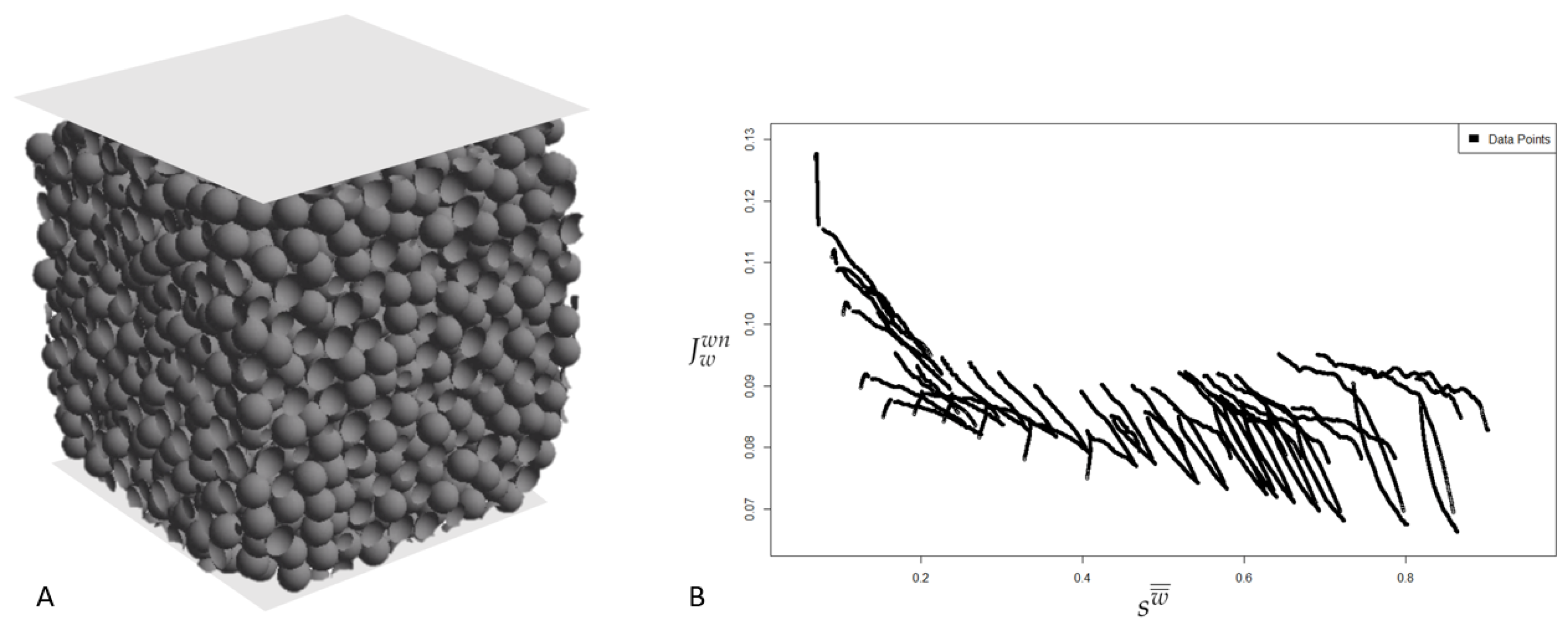
59]. One of these media is the classic Finney sphere packing, an ideal medium comprised of 4021 uniform spheres packed to a porosity of 0.369 as shown in
Figure 2 [
62]. The data from this set of simulations is publicly available and contains macroscale data for 54,341 unique fluid arrangements, a summary of which is also shown in
Figure 2. These arrangements include 20 near-equilibrium points along the primary drainage curve that were relaxed from points obtained with a morphological pore opening approach [
63]. Each near-equilibrium point is followed by pressure driven dynamic main imbibition and dynamic secondary drainage curves. The simulations were run with a lattice Boltzmann (LBM) simulator using a color model with a D3Q19 multiple relaxation time collision operator [
64,
65]. Comparisons of LBM to other microscale modeling methods are available in the literature [
66,
67]. The simulator solves the fluid distributions at the microscale and averages these values to produce averaged state quantities that arise in macroscale TCAT models [
68,
69].
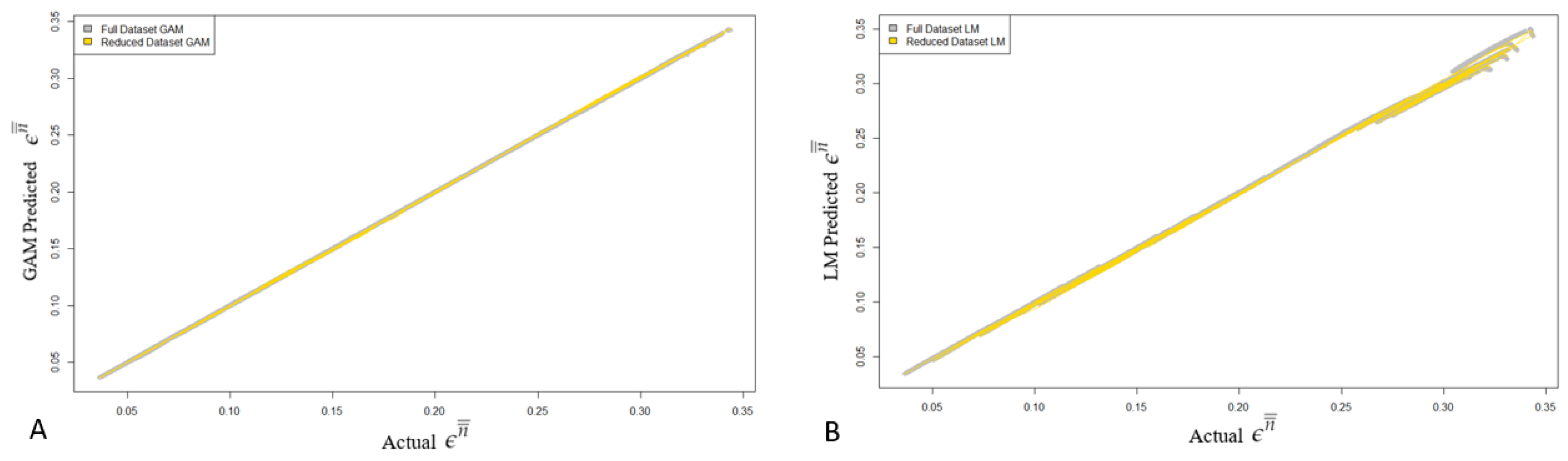
A global linear model (LM) and a GAM were both fit to the reduced 125 point data set. These two model types were chosen as they are significantly different in terms of complexity, are simple to implement, and can each be bolted into a macroscale simulator. The two fits were used to predict the non-wetting phase volume fraction over the entire state space consisting of 54,341 points using the interfacial areas, interfacial curvatures, and specific Euler characteristic. The fidelity of the two reduced data set fits are shown in comparison to the original fits on the entire data set in
Figure 3, where the reduced GAM is nearly indiscernible from the full GAM fit and the reduced LM also performs well.
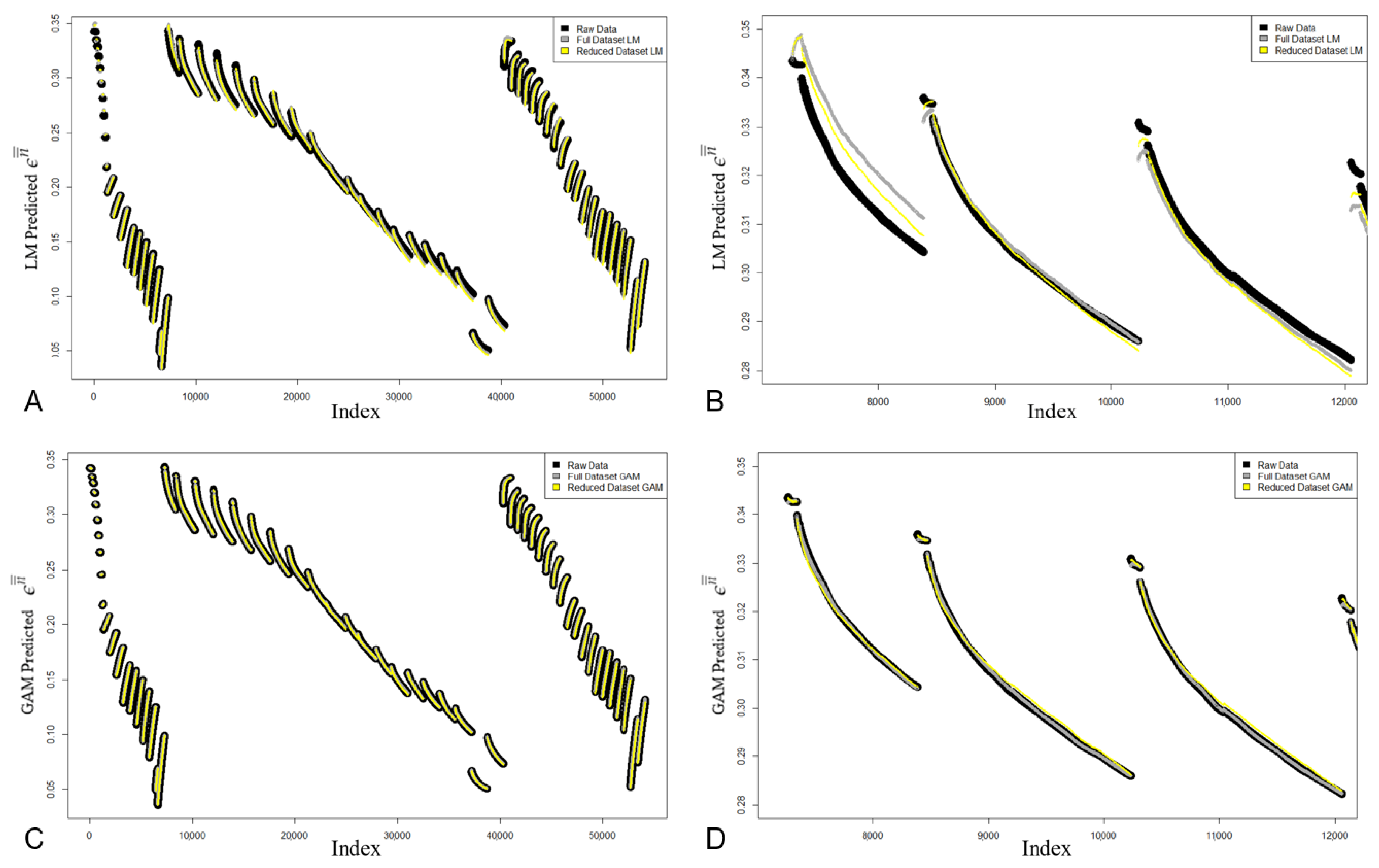
The high-quality of these fits can be qualitatively examined in more detail by considering the result at each point within the full data set as shown in
Figure 4. In sub-figures A and C, the 20 primary drainage relaxations are shown at indices less than 7264, imbibition curves are between indices 7264 and 40,309, and secondary drainage curves are greater than 40,309. Sub-figures B and D show only the first three stmain imbibition curves from sub-figures A and C where it can be seen that the reduced LM performs well compared to the full LM, and the reduced GAM is again nearly indistinguishable from the full GAM.
A quantitative comparison between each of the full and reduced model fits with the raw simulation data also demonstrates the excellence of the reduced form considering the 99.8% decrease in data points used to produce the model. A squared error (
) was taken between each actual non-wetting phase volume fraction and the predicted values from each of the four models where
in addition, the overall standard error of the estimate (
) was taken with
where
N represents the total sets of values being compared.
minimums, maximums, and quartiles and the overall
for each LM and GAM are given in
Table 1.
Points along primary drainage curves are relatively inexpensive to obtain when considering the morphological pore opening approach, however, simulations of imbibition to near-equilibrium states are time-consuming to compute with the LBM approach used in this work. A method to predict capillary pressure and saturation imbibition curves without the need for expensive simulations has been proposed [
70]. Combining this method with an LBM relaxation step as was performed for drainage could reduce the computational cost of producing these model fits to a nearly trivial amount. Augmentation with a set of random initialized states and dynamic data would be inexpensive to compute and likely important for cases outside the traditional bounds of primary drainage and main imbibition.
5. Resistance Coefficient State Equations
Examination of Equation (
2) shows a different form for the momentum approximation than what is typically expressed for the traditional model where relative permeabilities are used [
6,
71]. Three resistance coefficients must be determined for the TCAT model, which are the terms denoted by
. As we have shown to be the case with capillary pressure, we posit that a state equation also exists for these coefficients. We further posit that these equations will depend upon the same set of invariants as capillary pressure as the dependence of relative permeability on the morphology of the fluid phases is known to exist [
72,
73]. While the relationships between the Minkowski functionals and relative permeability have been explored, a state equation has not yet been proposed [
74].
We investigated our hypothesis with the same Finney packing data set as was used in the capillary pressure state equation analysis. It should be noted that while the two fluids within these simulations are immiscible, their densities and viscosities are equivalent to each other. We first consider Equation (
2) for the non-wetting phase under the assumption that gradients in volume fraction are small and therefore the
term can be neglected. This is done out of necessity, as the data set does not include the required quantities to evaluate the gradients. Reducing the form to the
z direction, ensuring the retention of the gravity term, we obtain
where the two resistance coefficients are to be fit simultaneously in linear form as
and
or in a nonlinear form as
and
where
and
are constants. In contrast to the capillary pressure analysis, the data set has been left in dimensional form and all reported values are in generic LBM units. Conversions between LBM and physical units can be performed with the following factors for length (L), density, and time (T)
and
For the full set of 54,134 states the LM represented by Equations (
13)–(
15) produces a fit with an
of 0.9430 while a natural spline (NS) fit represented by Equations (
13), (
16) and (
17) increases the
to 0.9634. An NS fit was implemented instead of the previously used GAM out of necessity as an eight parameter GAM over tens of thousands of data points is intractable. Neither fit performs particularly well, and we consider the alternative case that the term dropped from the momentum equation is significant for the accurate prediction of dynamic data and that improved results can be obtained by reducing the data to only near-steady state configurations where the volume fractions are essentially constant. We reduce the full data set by taking the final point from each of the 20 main imbibition and secondary drainage runs for a total of 40 fluid configurations.
LM and NS fits for the near-equilibrium and near-steady state data improved for the LM to an
of 0.9998 and the NS fit increased to an
of 1.0, indicating that our conjecture of the final term in the momentum equation being significant for dynamic data could be reasonable. The reduced data set LM and NS fits are shown in comparison to the raw data in
Figure 5. The coefficients for
and
in each LM are given in
Table 2. The wetting phase version of Equation (
13) produces the same result.
6. Discussion
We have formulated an example instance from a new generation of two-fluid-flow models. This formulated model has the potential to resolve many of the long-standing shortcomings associated with the traditional model, including the removal of hysteresis, non-wetting phase entrapment models, irreducible wetting-phase saturations, a reliance on assumptions of an equilibrium state, and a lack of connection with the microscale. Furthermore, interfacial areas and curvatures are naturally evolved with the model, and the interfacial tension between the fluid phases appears explicitly in the model.
Capillary pressure is shown to enter a state equation that is derived from theory. Because this is a new state equation form, many questions remain regarding the parameterization of this state equation. We consider approaches to determining a specific form of this state equation, and we show that an excellent representation of the system can be achieved with a small amount of data. This is a major advancement compared to the traditional model, which is based upon an assumption of equilibrium conditions which are difficult and time consuming to obtain using standard experimental approaches [
22]. Additional work should be done to repeat this analysis for different real and ideal media.
Other components are needed to reduce this new model to practice. One of these components is the determination of resistance coefficients. We use microscale data obtained from LBM simulations to examine the hypothesis that topological state equations exist for these coefficients. Because these simulations were not performed with this application in mind, the data set did not include every desirable quantity and it was necessary to drop the gradient of volume fraction term from the state equation model. By considering a small subset of the data for which volume fractions were nearly constant, excellent fits to a posited state equation were obtained. These results support the possibility that a state equation exists for the resistance coefficients and supports the need for additional study to test this hypothesis definitively with data sets that were designed for this purpose.
Further work is needed to complete the formulation of this new model. Specifically, expressions are needed for
and for
. Equations for both of these quantities can be derived using the averaging theorems, as was done for the evolution equations [
44]. The completion of these formulations and their validation is work that is in progress. We expect the completion of this work will provide the basis for a new class of high-fidelity simulator that resolves the many well-known limitations associated with the traditional model. Replacing an approach that has evolved over nearly a century is not trivial and considerable additional work will be needed to reduce this TCAT model to routine practice. Many may find that the traditional model is adequate for their needs and will not be early adopters. Many have expressed interest in this new class of models and understand the challenges associated with developing a new simulator consisting of a set of coupled equations and novel parameters needed for closure. Comparisons of the TCAT model with challenging macroscale data sets should be undertaken as a future evaluation.


