Article

Sliding Mode Switch Control of Adjustable Hydro-Pneumatic Suspension based on Parallel Adaptive Clonal Selection Algorithm

School of Mechanical and Aerospace Engineering, Jilin University, Changchun 130022, China
*
Author to whom correspondence should be addressed.
Appl. Sci. 2020, 10(5), 1852; https://doi.org/10.3390/app10051852
Submission received: 18 January 2020 / Revised: 26 February 2020 / Accepted: 4 March 2020 / Published: 8 March 2020
(This article belongs to the Section Mechanical Engineering)

Abstract

:
The hydro-pneumatic suspension, as a widely used suspension for heavy vehicles, has been taken seriously by researchers for a long time because it is crucial in terms of handling stability, riding comfort, and driving safety of these vehicles. Most previous studies only discussed the control of ride comfort or vehicle handling stability of the suspension system separately. This article proposes a dynamic switch control strategy which can switch between ride comfort and handling stability controllers under different road surfaces and driving conditions. The load transfer ratio (LTR) is selected as the switch performance index, and it is calculated through a six-degrees-of-freedom (6-DOF) model. The ride comfort and handling stability controller of the hydro-pneumatic suspension are designed based on the sliding mode control theory. The objective functions of parameters optimization of the sliding mode controller (SMC) are obtained by means of analytic hierarchy process (AHP), and then the controller’s parameters are optimized by the parallel adaptive clonal selection algorithm (PACSA). The simulation results based on MATLAB/Simulink show that: (1) the PACSA performs better than a genetic algorithm in terms of the parameters optimization of the SMC; (2) the proposed switch control strategy can simultaneously improve the ride comfort and handling stability under several typical steering maneuvers and various road profiles compared with the conventional SMC-controlled suspension.

1. Introduction

Rescue vehicles are important in the transportation of rescue goods as well as rescue workers. The hydro-pneumatic suspension is applied to rescue vehicles due to the great load carrying capacity and the complexity of rescue terrain. The hydro-pneumatic suspension system plays a decisive role in the ride comfort and handling stability of the vehicle, but the passive suspension cannot address various road profiles because of its fixed parameters. As a result, it is meaningful and feasible to study a control strategy for the adjustable hydro-pneumatic suspension system which can perform better in ride comfort and handling stability than the traditional passive suspension [1].
In previous studies, many scholars have studied the control strategy of the adjustable hydro-pneumatic suspension. Andres Riofrio [2] improved the vehicle rollover stability of active suspension through an LQR (linear quadratic regulator)-based controller with estimation of the road. Shuai Wang [3] discussed the active control of hydro-pneumatic suspension parameters of wheel loaders based on a fuzzy controller, which reduces the vertical vibration of the wheel loader. Sarel F [4] presented the possibility of using slow active suspension control to reduce the body roll and thus reduce the rollover propensity. Awad, Magdy Naeem [5] designed a hydro-pneumatic energy harvesting suspension system based on a PID-PSO (particle swarm optimization) controller, which achieved the maximum riding comfort as the peak values of the acceleration.
However, past research on adjustable hydro-pneumatic suspension mainly focused on the analysis of vehicles’ ride comfort or handling stability under different operating conditions separately, because it is difficult to achieve optimality in both aspects of ride comfort and handling stability due to the conflicting relationship between them. Hence, it is urgent to concentrate on the dynamic switch control strategy between the vehicle’s ride comfort and handling stability to meet different requirements of working conditions.
As a powerful controller, the sliding mode controller (SMC) has a great use in control systems because of its good robustness to external disturbance and fast dynamic response. Pradhan, Subarni [6] applied a composite SMC for wind power extraction in a remotely located solar PV-wind hybrid system. Biricik, Samet [7] used an SMC three-phase dynamic voltage restorer with adaptive notch filter to protect sensitive loads. Farahmandrad, Maryam [8] designed a fuzzy SMC for a cooperative robotic system with uncertainty for handling an object. Abtahi, S. Mahdi [9] suppressed chaotic vibrations in a suspension system of vehicle dynamics based on the optimal SMC. Inspired by the previous studies mentioned above, an SMC is used to control the hydro-pneumatic suspension system to enhance the ride comfort and handling stability of the rescue vehicle in this paper.
Parameters of SMCs should be tuned suitably to achieve the optimal control effect. At present, many optimization methods are used in SMCs, for example, particle swarm optimization (PSO) [10], Genetic Algorithm (GA) [11], and adaptive clonal selection algorithm (ACSA) [12,13,14,15]. PSO has relatively fast convergence speed, while it is easy to fall into local optimal solution, and it is unstable. GA is able to get the global optimal solution based on the natural evolution principle, but it has the shortcomings of longer calculation. ACSA has received increasing attention as one of the approaches to optimize parameters, due to its highly adaptive and easy-to-implement nature [12]. Maryam Sadat Hashemipour [13] used ACSA to optimize the support vector machine parameters and feature subset selection. Liang Hongtao [14] presented a novel objective optimization approach based on ACSA to solve the problems of weapon-target assignment in warship formation antiaircraft application. B. Srinivasa Rao [15] proposed a new multi-objective optimization approach by means of the ACSA to solve a complex environmental/economic dispatch problem of thermal generators in power systems. PACSA is proposed on the basis of ACSA, where ’P’ stands for the parallel computing which can greatly reduce the running time of optimization operations through sacrificing hardware resources [16,17]. In this article, PACSA is used to tune the parameters of the SMC, which combine the ACSA with parallel computing to improve the efficiency of the system.
In this paper, an adjustable hydro-pneumatic suspension system of a rescue vehicle is taken as the object to study the proposed dynamic switch strategy between the ride comfort and handling stability. The load transfer ratio (LTR) is selected as the switch performance index, and it is calculated through a six-degrees-of-freedom (6-DOF) model. The ride comfort and handling stability controller of the hydro-pneumatic suspension are designed based on the SMC. The objective functions of parameters optimization of the SMC are obtained by means of analytic hierarchy process (AHP), and then the SMC’s parameters are optimized by the PACSA.
The research of the adjustable hydro-pneumatic suspension in this paper has highlights as follows.
(1)
The 6-DOF model of the adjustable hydro-pneumatic suspension based on the rescue vehicle is established, and the sliding mode controller is applied on the rescue vehicle because of its robust and easy realization.
(2)
A Switched SMC is proposed and built for the control of the adjustable hydro-pneumatic suspension system, which can address concerns on both ride comfort and handling stability under different road surfaces and driving conditions through switch actions, and the optimization ability of the proposed control strategy is proven compared with the conventional SMC based on MATLAB/Simulink.
(3)
PACSA is used to optimize the parameters of the Switched SMC, which is verified as more suitable for tuning the parameters of the SMC controller.
The rest of this paper is organized as follows. Section 2 establishes the road model and the 6-DOF half-car model of the suspension system. Section 3 focuses on the switch control strategy of the hydro-pneumatic suspension. Section 4 describes the parameter tuning methods of the SMC. Section 5 carries out the simulation of the designed controllers, and the simulation results are analyzed. Section 6 is the conclusions.

2. System Modelling

For the controller design and the validation of the switch control strategy, the models of the hydro-pneumatic suspensions system, nonlinear tire input, and road input are established in this section.

2.1. Modelling of the Hydro-Pneumatic Suspension System

The vehicle studied in this paper is a rescue vehicle with an adjustable hydro-pneumatic suspension system. The corresponding model has six degrees of freedom which represent the vertical, roll, and lateral dynamics of the vehicle. The 6-DOF model consists of two parts, one is a 4-DOF roll motion model (Figure 1a) and the other is a 2-DOF steer-yaw model (Figure 1b). The 4-DOF roll motion model comprises a lumped spring mass, and two unspring masses are developed. The 4-DOF are composed of the translational motions in the vertical direction of the spring mass and the two unspring masses and the roll motion of the spring mass. The 2-DOF of the steering model consist of the lateral and yaw motions of the vehicle.
For convenience, we give the linear approximation for the damping and stiffness of the hydro-pneumatic suspension by fitting, and the fitted stiffness and damping of the suspension are shown in Table 1. In addition, two tires are modeled by means of two linear springs. The parameters of the rescue vehicle’s suspension system are displayed in Table 1.
According to Figure 2 and Newton’s law, the dynamic motions of the rescue vehicle are modelled as follows.
Rolling dynamic motion:
I x φ ¨ = T [ ( F l + f u l ) ( F r + f u r ) ]
Lateral motion:
m s v x ( β ˙ + γ ) = F f y F r y m s g φ
Yaw motion:
I z γ ˙ = F f y l f _ F r y l r
where φ , γ , β represent the roll angle, yaw rate, and side-slip angle, respectively; v x is the speed of the vehicle;
Vertical motion equation of the spring mass:
m s z ¨ s = F l + F r + f u l + f u r F l = c s ( z ˙ u l z ˙ s l ) + k s ( z ˙ u l z ˙ s l ) F r = c s ( z ˙ u r z ˙ s r ) + k s ( z ˙ u r z ˙ s r )
where z s denotes vertical displacement of sprung mass; f u l and f u r indicate the adjustable control forces of the suspension.
Vertical motion equation of the unspring mass:
m u l z ¨ u l = k t ( z q l z u l ) F l f u l m u r z ¨ u r = k t ( z q r z u r ) F r f u r
where z s l = z s + T φ z s r = z s T φ , z q l , z q r indicate the vertical displacements of the wheels excited by the road surface, z u l , z u r is the vertical displacements of unspring mass. The subscript l and r of the symbols represent the left and right suspension.

2.2. Tire Model

The tire mechanics property plays a vital role in the vehicle’s dynamics performance, handling stability and comfort. The vertical dynamics and lateral dynamics of the vehicle are coupled to each other by the tire force; hence, the accuracy of the tire model is essential. Tire models are usually divided into theoretical models and empirical or semi-empirical models according to their structural points. The empirical tire is generated based on a large number of experimental data fittings [18], and it is generally accurate, as for example, Pacejka’s tire model. Fiala and UA tire belong to the theoretical tire model, which is inaccurate but physically meaningful [19]. WEI Yintao [20] proposed that the theoretical physical model is impossible to practically apply to automobile dynamics simulations because it lacks the accuracy of quantitative description. Yasheen Babulal [21] parameterized three existing tire models namely, Fiala, UA, and Pacejka tire models, and he drew a conclusion that the Pacejka tire model tire provided the closest fit for the side-force versus slip angle tests of all three tire models.
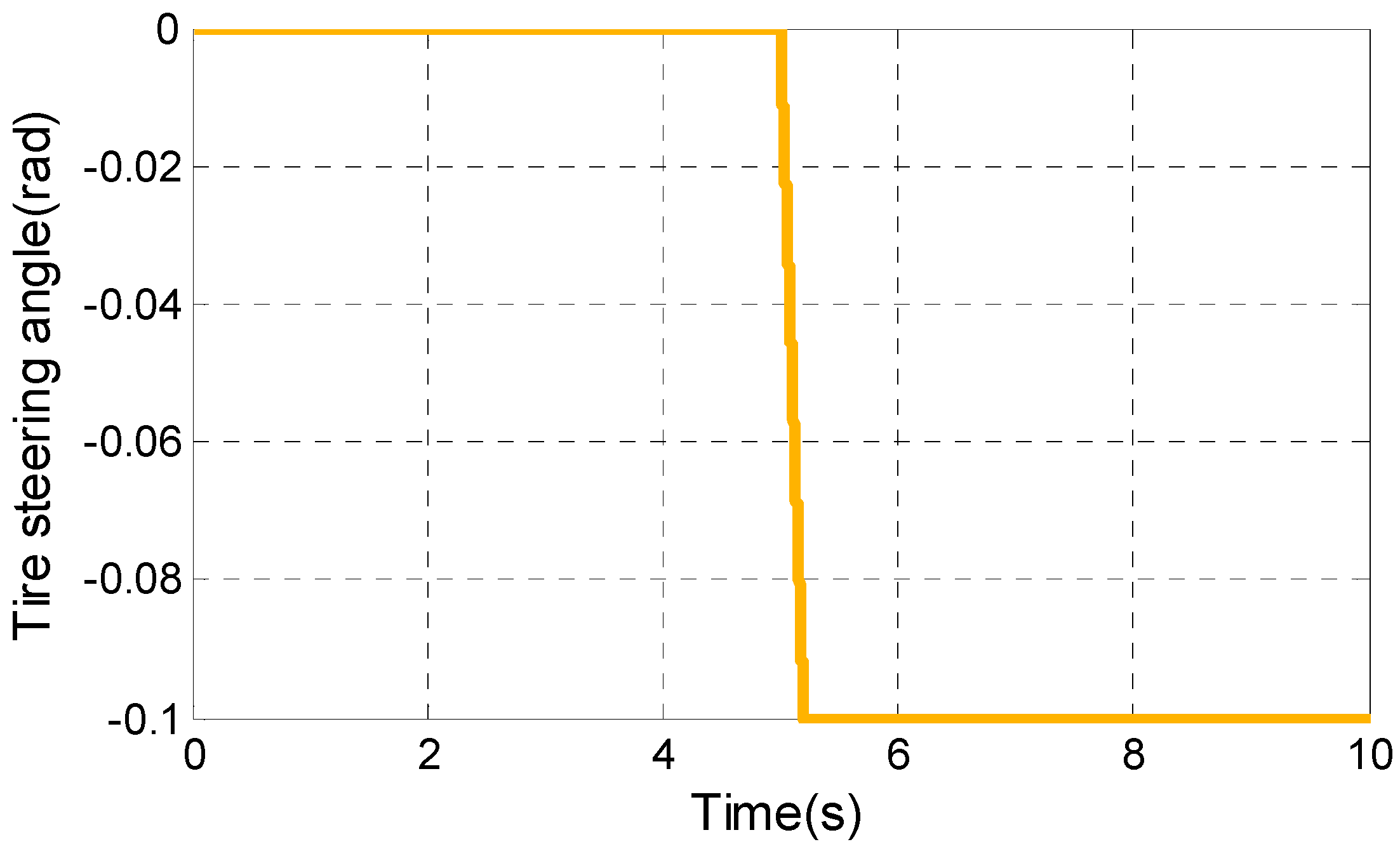
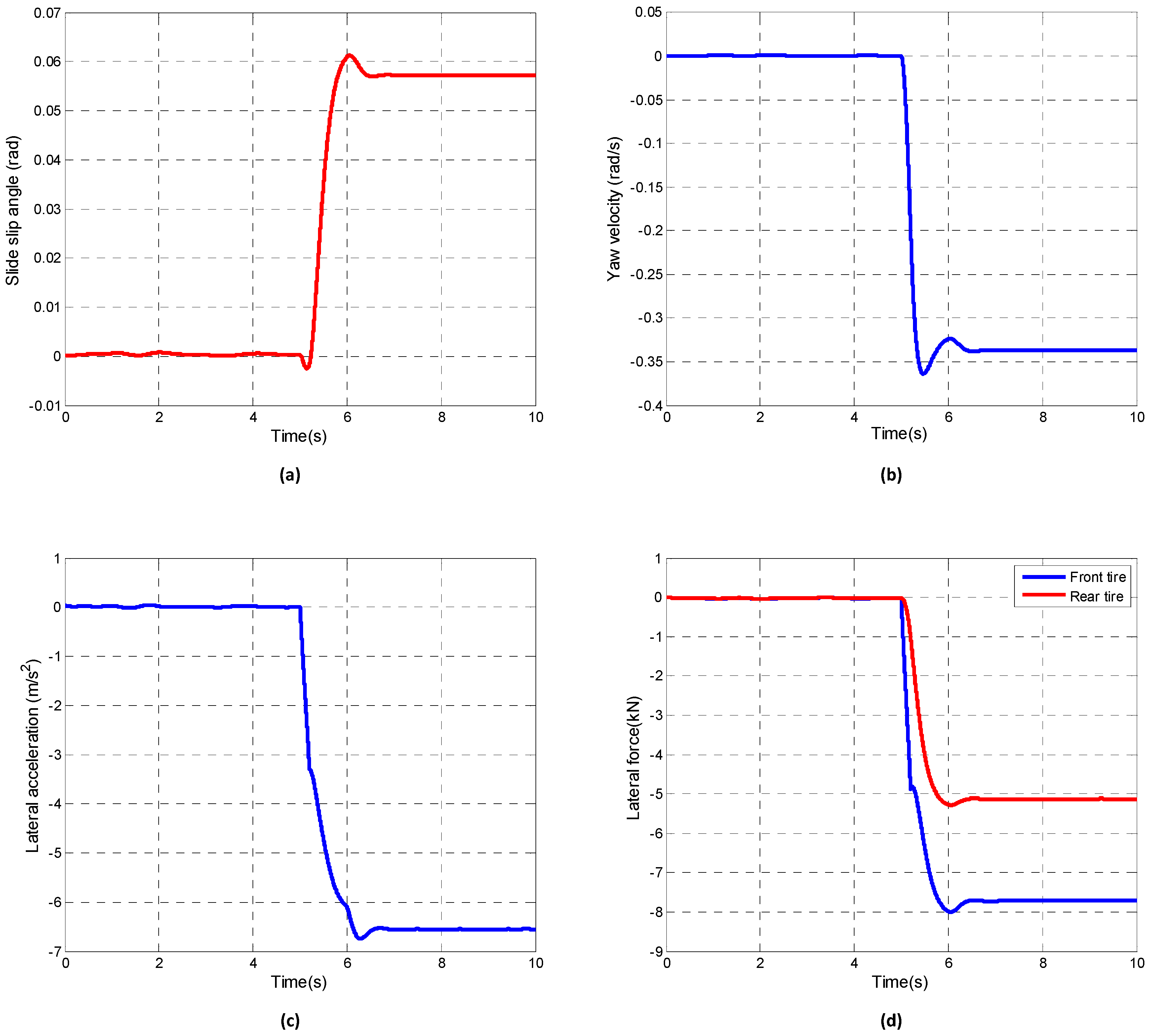
The Pacejka tire model shows the relationship among the longitudinal force, the lateral force, the aligning torque and the side angle. It has a high fitting accuracy and can be used within a certain range except for extreme conditions. Therefore, the Pacejka tire model is selected in this paper to calculate the tire lateral force coupled with the vertical load. The relevant expression of the tire model can be found in Ref [19]. The Pacejka tire model is established in MATLAB/Simulink, and the correlative curves under the steering condition of Figure 2 are shown in Figure 3.
It can be seen from the tire simulation results in Figure 3, the values and the trend of curves are consistent with the curves in Ref [22], which illustrates the correctness of the tire model established in this article.

2.3. Road Input Modelling

All analyses and studies of the suspension system are implemented on the basis of the input of the stochastic road surface, because the excitation of road wave surface is the main vibration source of the vehicle vibration system [23]. Accurate road models are important to the research and optimization of the suspension system. Random road surface is generally selected as the most commonly used in simulation, and more results and significance can be obtained in Ref [24]. The expressions of z q l , z q r are shown in Equation (6).
z ˙ q l ( t ) = 2 π f 0 z q ( t ) + 2 π n 0 w ( t ) G q ( n 0 ) v x z q r ( t ) = [ 1 0 ] [ X 1 X 2 ] + z q l ( t ) [ X ˙ 1 X ˙ 2 ] = [ X 2 12 v x T z q l ( t ) 12 v x 2 T 2 X 1 6 v x T X 2 + 72 v x 2 T 2 z q l ( t ) ]
where w ( t ) is white noise signal of the road, and f 0 = v x × n 00 . X 1 and X 2 are the state variables in the state equation.
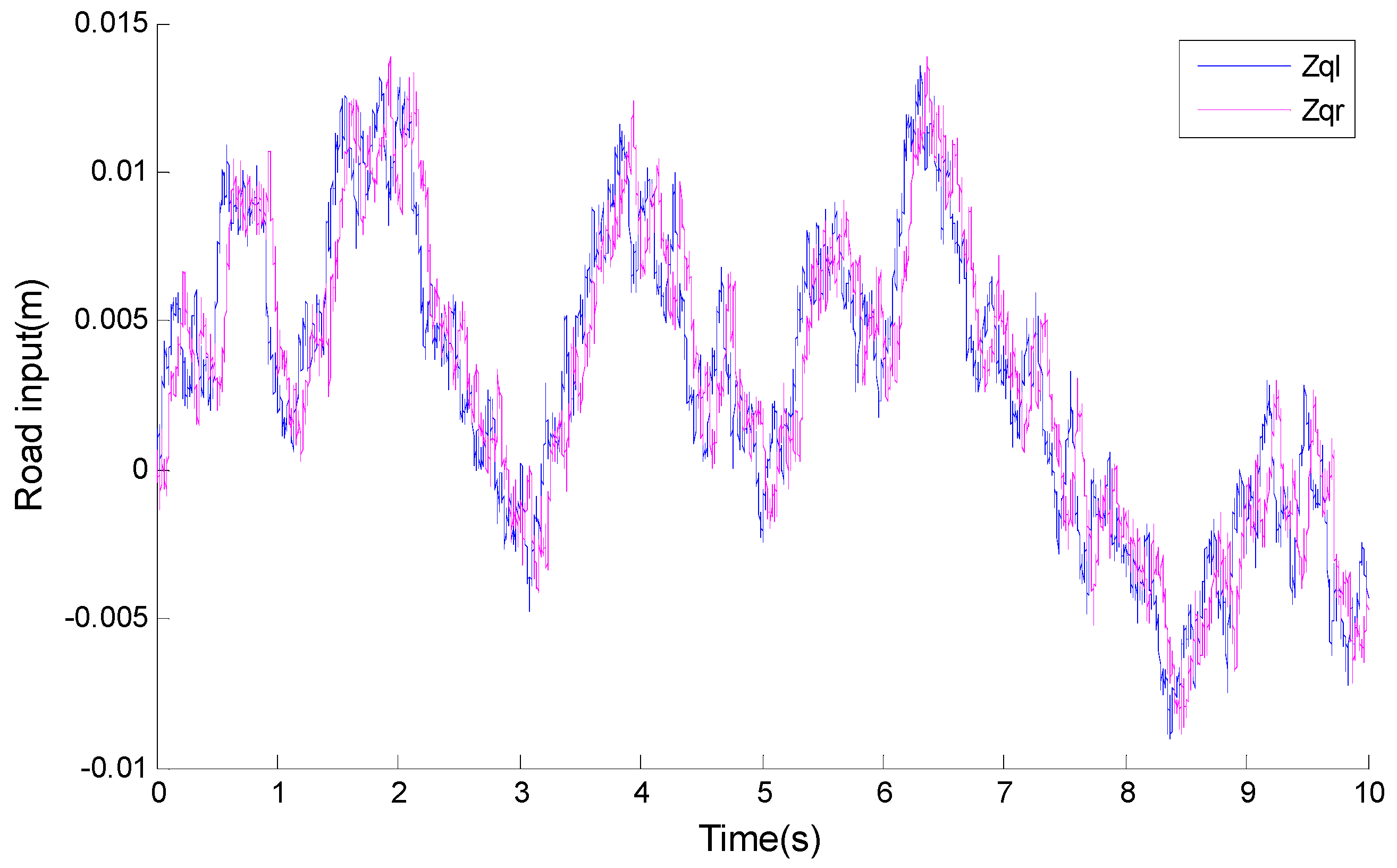
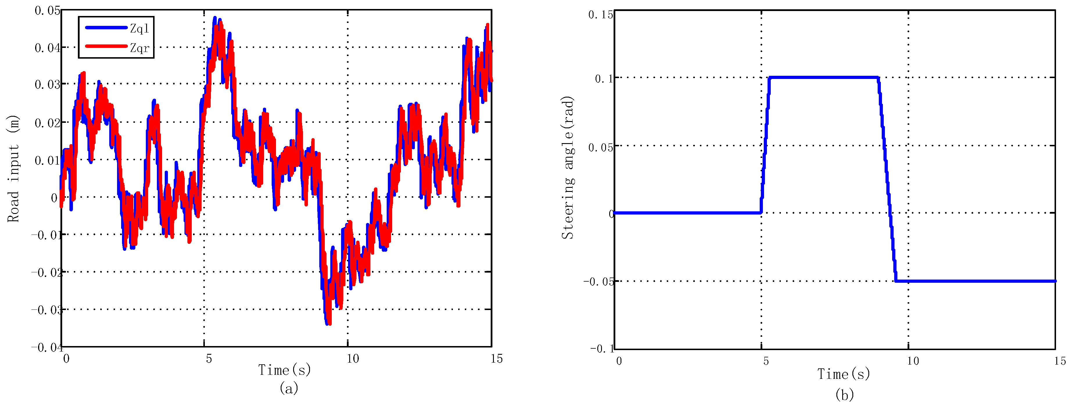
The random road model is established based on MATLAB/Simulink, and the simulated displacement curves of the left and right tires are shown in Figure 4, where n 0 = 0.1 m 1 , f 0 = 0 . 011 m 1 , n x = 70 k m / h , G q ( n 0 ) = 0.016384 m 3 .

3. The Switch Control Strategy of the Hydro-Pneumatic Suspension

3.1. Switch Control Strategy

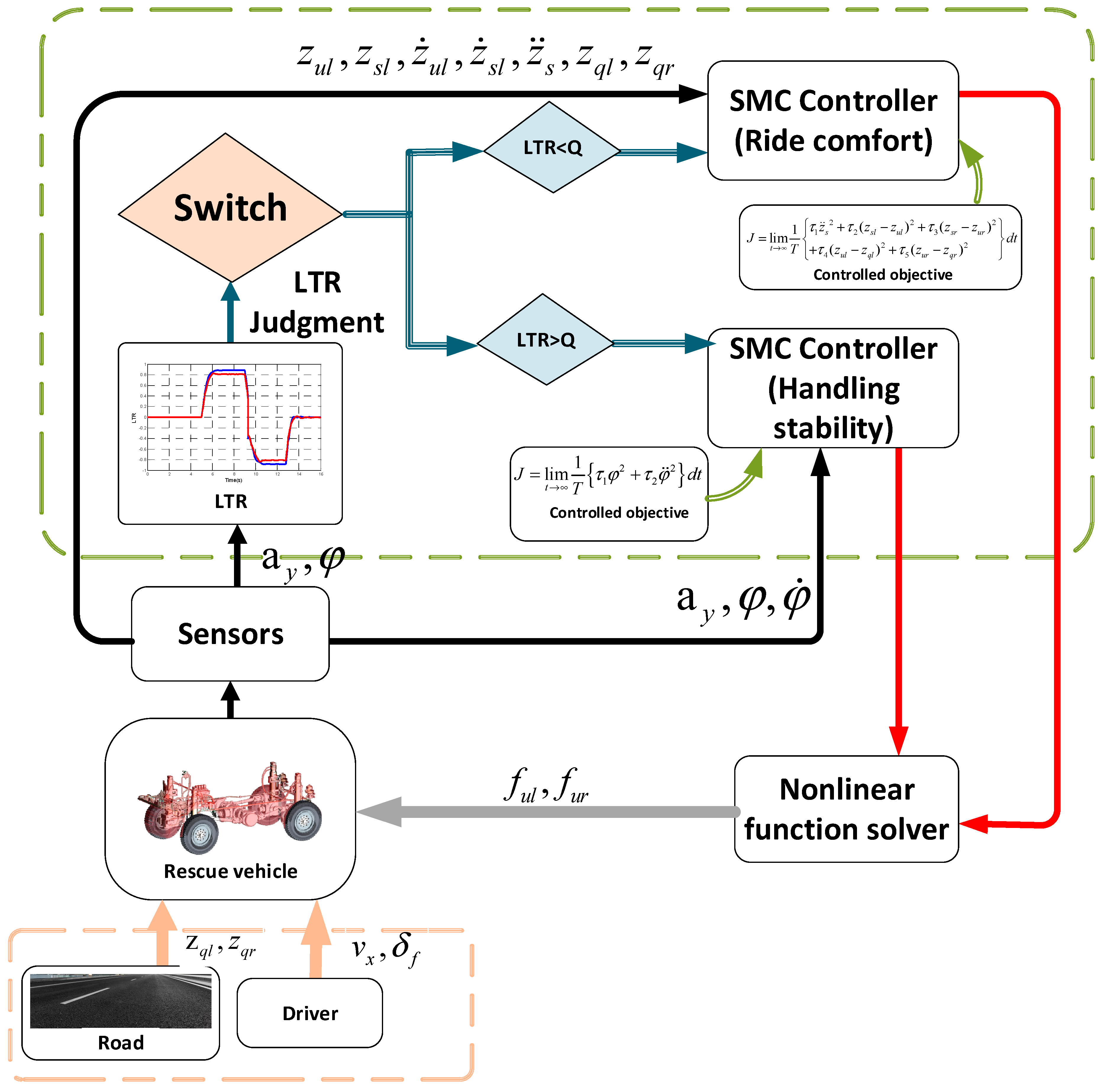
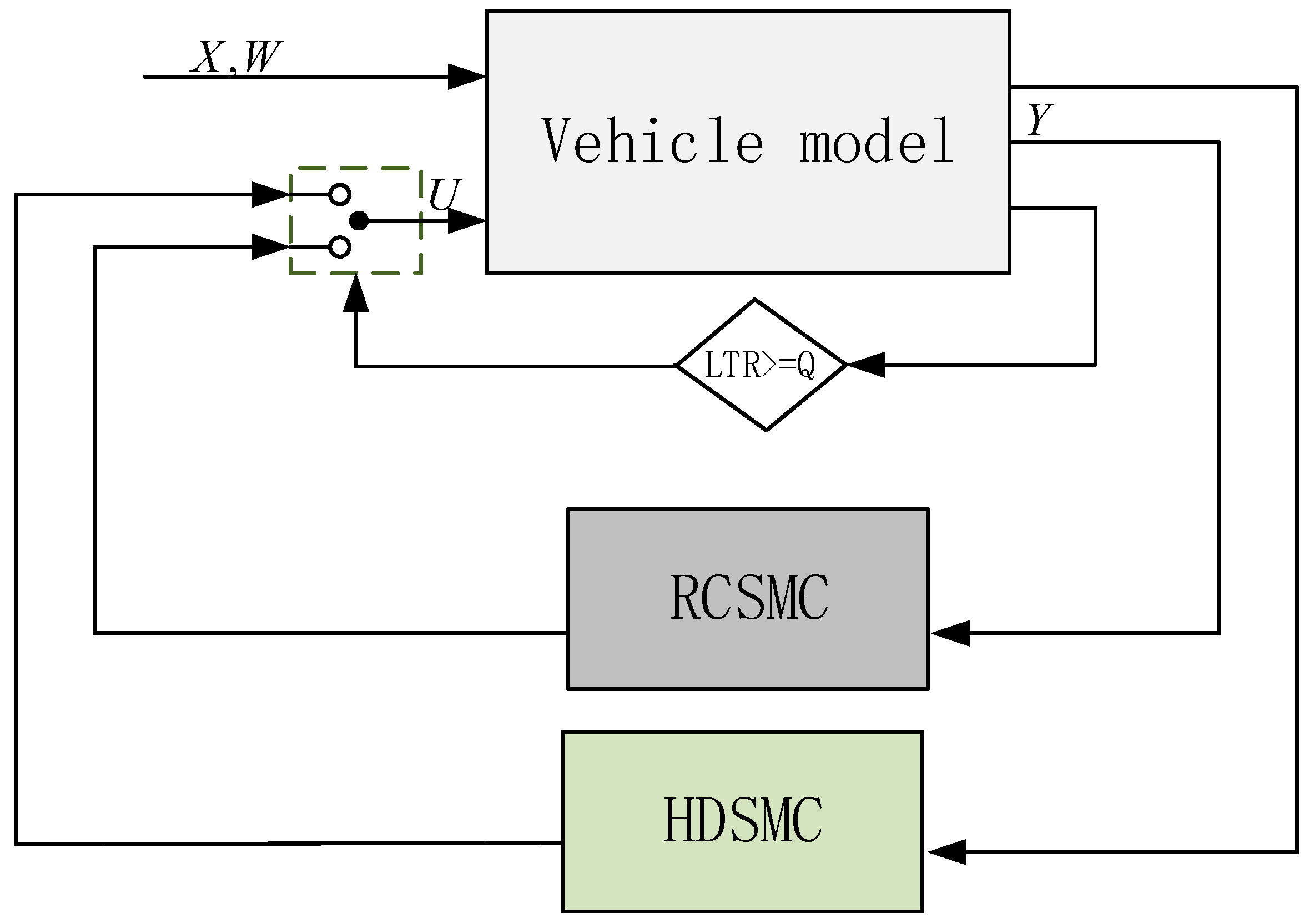
Based on the conflicting relationship between them, it is difficult to optimize both aspects of ride comfort and handling stability of the rescue vehicle based on the control of the hydro-pneumatic suspension. However, when the vehicle is in different driving conditions or driving on different road surfaces, level of magnitude of the two aspects can be sorted. For instance, when the road surface is relatively flat and the driving state of the vehicle is unlikely to cause the vehicle to be dangerous, the ride comfort is the main goal pursued by the suspension system in this case. On the contrary, when the vehicle is driving on an uneven road or steering at a high speed, the possibility of rolling of the vehicle is relatively large at this time, and the handling stability of the vehicle is the major demand of the vehicle. As a result, it should be possible to analyze the weight of the vehicle’s ride comfort and the handling stability under different conditions, so as to achieve the corresponding switch according to different requirements of working conditions. For the above-mentioned idea, the switch control strategy is presented in this paper, and the schematic diagram of the switch control strategy of the hydro-pneumatic suspension is shown in Figure 5.
where δ f is the steering angle of the wheel, and a y is the lateral acceleration of the spring mass, a y = v x ( β ˙ + γ ) .
For the switch control strategy, an indicator is needed to determine whether and when the switch occurs. In order to evaluate the possibility of the vehicle’s danger, LTR is selected as the performance index to judge whether the switch action between the ride comfort and handling stability controllers is triggered, and LTR is defined as follows.
L T R = 2 m s m T ( ( h r + h cos φ ) a y g + h sin φ )
When the LTR is equal to 0, the vehicle has a stable roll dynamic, and the risk becomes higher with the increase of LTR [25]. The threshold of LTR is defined as Q, then the switch control strategy can be illustrated in Equation (8). In order to ensure sufficient time for the controller to react before the rollover danger occurs, Q is set to 0.8 in this paper. On this occasion, the controller has enough time to lower the LTR to avoid the rollover before obtaining high values of LTR.
c o n t r o l l e r = { r i d e c o m f o r t c o n t r o l l e r , L T R Q h a n d i n g s t a b i l i t y c o n t r o l l e r , L T R > Q
In order to easily understand the proposed control strategy, the control block diagram of the switch control strategy of the hydro-pneumatic suspension is shown in Figure 6. As shown in Figure 6, when the value of LTR is lower than Q, it indicates that the vehicle is not at risk of rollover at this time. As a result, the major task of the controller is to optimize the ride comfort of the suspension system, then the ride comfort SMC (RCSMC) is active. The handling stability SMC (HDSMC) is not activated until the LTR reaches the threshold Q.

3.2. Handling Stability Control

Once the gravity center of the heavy vehicle is laterally offset owing to severe maneuvers, a centrifugal moment ( M c ) is generated, and the vehicle is at risk of rolling over. The actuator of the adjustable hydro-pneumatic suspension can generate a torque ( M t ) against the centrifugal moment under the appropriate control of the controller, thereby preventing the vehicle from rolling over. Consequently, the following vehicle roll dynamic model is obtained.
I x φ ¨ = T ( F l F r ) + m s a y h + M c M t + κ M c = m s g h sin φ , M t = f u l T
where κ represents the allowable uncertainties, and κ κ 1 | φ | + κ 2 | φ ˙ | . Both κ 1 κ 2 are positive constants.
As we can see from Equation (9), the system input is M t , and the output is φ . From SMC theory, the sliding surface is defined as below.
s = ρ e + e ˙ = ρ φ + φ ˙
where ρ ( ρ > 0 ) indicates the performance of system converging to the equilibrium point. e is the difference between the ideal output and actual output, and the ideal output of the roll angle is zero, in other words, e = φ .
For the purpose of effectively improving the asymptotic stability and decreasing chattering aroused from SMC’s switch characteristic, the exponential reaching law is selected to converge towards 0 exponentially in this paper, which is rewritten in Equation (11).
s ˙ = μ sgn s η s
In order to satisfy the Hurwitz criteria [26], Equation (12) is selected as the Lyapunov candidate function, which is strictly negative. Equation (13) should be satisfied to ensure the robustness stability of the controller.
V = 1 2 ( e 2 + s 2 )
η > κ 2 μ > ( 1 + κ 1 + κ 2 ) φ max
where μ and η are the coefficients that represent the speed reaching the sliding surface, μ > 0 η > 0 .
According to Equations (10)~(13) mentioned above, the control input can be rewritten as Equation (14).
f u l = - f u r = I x ( μ sgn s η s ρ φ ˙ ) ( F l F r ) m s a y h + m s g h sin φ + κ T

3.3. Ride Comfort Control

Through many years of investigation and practice, the quarter-car suspension nonlinear model is suitable for the research on the ride comfort control [27]. In this paper, the ride comfort controller of the hydro-pneumatic suspension is built based on the quarter-car model, which makes it easy to compute. Through this quarter-car model, the controller output ( f u l ) of one side of the suspension can be calculated, and the other side controller output is expressed as f u r = ζ f u l , where ζ is the correlation coefficient that connects the control quantity of left and right sides’ suspensions. The value of ζ can be obtained through the optimization algorithm which will be introduced in the Section 4. According to Newton’s law, the state space representation can be written as follows.
{ X ˙ = A X + B U + G W Y = C X + D U
where
X = [ z u l z s z ˙ u l z ˙ s ] T , U = f u l , W = z q l
A = [ 0 0 1 0 0 0 0 1 k t + k s m u k s m u c s m u c s m u k s m s k s m s c s m s c s m s ] , B = [ 0 0 1 m u 1 m s ] , G = [ 0 0 k t m u 0 ]
C = [ 1 0 0 0 0 1 0 0 0 0 1 0 k s m s k s m s c s m s c s m s ] , D = [ 0 0 0 1 m s ]
Define the sliding surface as
S ( X ) = n 1 x 1 + n 2 x 2 + n 3 x 3 + x 4
where X is the state vector, and the polynomial p 3 + n 3 p 2 + n 2 p + n 1 should satisfy the Hurwitz law based on the design criteria of the SMC. [28] On the basis of modern control theory, the variable structure systems’ controllability should be constant for any nonsingular transformation. Because of the controllability of the matrices A and B , the nonsingular transformation is carried on X .
X ˜ = T s X
[ X ˜ ˙ 1 X ˜ ˙ 2 ] = [ A 11 A 12 A 21 A 22 ] [ X ˜ 1 X ˜ 2 ] + [ 0 B 2 K 0 ] [ f u l z q l ]
The values of the matrices in Equations (17) and (18) are shown as follows.
T s = [ 1 0 0 0 0 1 0 0 0 0 1 m s m u 0 0 0 1 ] , X ˜ 1 = [ x 1 x 2 x ˙ 1 + m s m i x ˙ 2 ] , X ˜ 2 = [ x ˙ 2 ] A 11 = [ 0 0 1 0 0 0 k t m u 0 0 ] , A 12 = [ m s m u 1 0 ] , A 21 = [ k s m s k s m s c s m s ] A 22 = c s ( 1 m u + 1 m s ) , B 2 = 1 m u , K = [ 0 0 k t m u ] T
The sliding surface can be rewritten according to Equations (16) to (18).
S ( X ) = [ N 1 N 2 ] · [ X ˜ 1 X ˜ 2 ] = N 1 X ˜ 1 + N 2 X ˜ 2
where
N 1 = [ n 1 n 2 n 3 ] , N 2 = [ m u m u m s n 3 ] , m u m s n 3 0
X ˜ 2 = m u m s n 3 m u N 1 X ˜ 1 X ˜ 1 = ( A 11 A 12 N 2 1 N 1 ) X 1
For the purpose of satisfying the Hurwitz criteria to ensure the stability according to the SMC theory, Equation (21), the characteristic polynomial of Equation (20), should ensure the roots are negative. In other words, the value of p must be greater than zero. As a consequence, the bounds of n 1 , n 2 , and n 3 are confirmed, as shown in Equation (22).
λ 3 + m u n 2 m s n 1 m u m s n 3 λ 2 + k t m u m s n 3 λ + k t n 2 m u m s n 3 = 0
( λ + x ) 3 = λ 3 + 3 x λ 2 + 3 x 2 λ + x 3
{ m u n 2 m s n 1 > 0 m u m s n 3 > 0 n 2 > 0
Similarly, the exponential reaching law is also applied to the design of the ride comfort controller, and the controller output ( f u l ) can be obtained.
f u l = ( N T B ) 1 [ N T A X + μ sgn S ( X ) + η S ( X ) ]

4. SMC Parameters Tuning Based on PACSA

During the process of designing the SMC, parameters of SMC should be chosen suitably through some optimization algorithms to obtain optimal performance. For the RCSMC, there are six parameters that can be tuned, i.e., n 1 , n 2 , n 3 , η , μ , and ζ . Likewise, five related parameters of the HDSMC need to be optimized, which are ρ , μ , η , κ 1 , and κ 2 . In this section, two objective functions of parameters optimization are designed through AHP, and then the PACSA is applied to optimize the above parameters of the two controllers based on the objective functions.

4.1. Design of Objective Function based on AHP

4.1.1. Objective Function

Appropriate performance evaluation indicators are the basis for judging the quality of control strategies. Ride comfort and handling stability are the main aspects of vehicle performance during the running process of vehicle. In order to achieve optimal SMC of vehicle ride comfort and handling stability, the objective function of the SMC’ parameters optimization consists of vehicle vertical acceleration z ¨ s , dynamic deflection of left and right tire z q l z u l and z q r z u r , left and right side suspension dynamic deflection z u l z s l and z u r z s r , and roll angle acceleration of vehicle φ ¨ . The first three items are the objective function factors often used in suspension ride control [29,30]. The roll angle acceleration is the main control target in the handling stability control of the suspension system [31,32]. In order to trade off among the various performance requirements for better ride comfort and handling stability, a quadratic objective function expression is taken as the performance index based on the quadratic optimal control theory, which is shown in Equation (24).
J = lim t 1 T { τ 1 z ¨ s 2 + τ 2 φ ¨ 2 + τ 3 ( z s l z u l ) 2 + τ 4 ( z s r z u r ) 2 + τ 5 ( z u l z q l ) 2 + τ 6 ( z u r z q r ) 2 } d t
where τ 1 τ 6 are the weighting coefficients of the corresponding items.
First of all, the six weighting indicators mentioned above should be quantified because of the big differences in magnitude between them. The root mean square (RMS) value of the above six indicators in the passive suspension model is calculated, and the quantized scale factor of the same scale can be obtained from Equation (25).
γ 1 σ z ¨ s 2 = γ 2 σ φ ¨ 2 = γ 3 σ z s l z u l 2 = γ 4 σ z s r z u r 2 = γ 5 σ z u l z q l 2 = γ 6 σ z u r z q r 2
where γ 1 γ 6 are the quantized scale factors. The vertical displacement acceleration z ¨ s is used as a reference, and the value of γ 1 is set to 1. The calculation results are shown in Table 2.

4.1.2. Weighting Coefficient Optimization of the Objective Function based on AHP

The weighting coefficients have a great influence on the value of the objective function; therefore, it is essential to reasonably select the weighting coefficients of the objective function. In this study, the weighting coefficients are determined by AHP to avoid multifarious trial and error.
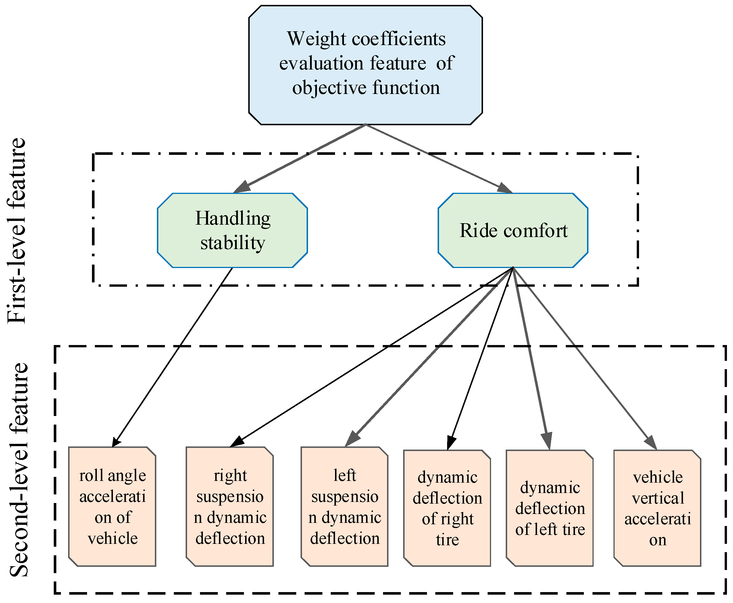
AHP is used for multi-criteria decision making in which the factors are arranged in a hierarchical structure [33]. The weight coefficients evaluation process of the objective function based on AHP is shown in Figure 7.
1. Set up hierarchical analysis model
The hierarchical analysis model is displayed in Figure 8, where the first level evaluation feature is composed of ride comfort and handling stability during the vehicle driving. The second level evaluation feature includes vehicle vertical acceleration, dynamic deflection of left and right tire, left- and right-side suspension dynamic deflection, and roll angle acceleration of the vehicle. Therefore, the structure of the hierarchical analysis model is derived from the objective function to acquire the priority of the evaluation feature on each level.
2. Construct judgment matrix T
The judgment matrix T is applied to distinguish the relative emphasis of evaluation features per hierarchical layer. T is constructed by using a nominal scale from 0 to 9 with the value a i j , which is assigned to express the relative importance of evaluation element a i over a j . The matrix T = { a i j } is established by the importance comparison between evaluation features.
3. Calculate weight vector corresponding to T
The weight vector can be written as Λ = ( τ 1 , τ 2 , , τ r ) T , where r denotes numbers of evaluation features per level. Λ is gained through the normalization process for judgment matrix T.
4. Consistency check of judgment matrix
Generally, CI (consistency index) is used to check the consistency deviation of the judgment matrix, whose expression is shown as follows.
C I = η max m m 1
where m represents the order of judgment matrix T . η max indicates the root of maximum eigenvector value. At the same time, the formula of η max is displayed as follows.
η max = i = 1 r ( T τ ) i r τ i
In addition, in order to check the consistency more effectively, CR (ratio of consistency check) is introduced as shown in the following equation.
C R = C I R I
where RI is the reference criterion, and Table 3 shows the value of RI. If the value of CR is less than 0.10, it means that the consistency check is qualified.
5. Calculate the weight of evaluation features per level
If the judgment matrix satisfies the consistency, then the weight of the evaluated feature on each level is the eigenvector obtained; otherwise, the eigenvector needs to be calculated. The weights of evaluation features on two levels can be calculated by means of the four steps mentioned above. If τ f i r s t = { ρ i } , τ sec o n d = { q j } , then the weight of the lowest level feature is described as follows.
τ i j = ρ i q j γ i
where τ i j represents the weight of jth feature at the second-level relative to the weight of ith feature at the first level. γ i is the quantization scale factor.
Above all, the weight coefficients of the objective function of the SMC’ parameters optimization in Equation (24) are shown in Table 4. It can also be seen from Table 4 that the vehicle vertical acceleration and the roll angle acceleration of vehicle are the two main factors which can reflect the ride comfort and handling stability of the vehicle, respectively. As a result, the two objective functions for the optimization of the RCSMC and HDSMC are shown in Equation (29).

4.2. Optimal Tuning Process of SMC based on PACSA

4.2.1. Brief Introduction of PACSA

The natural biological immune system has greatly influenced the development of computational intelligence in recent years, and many scholars have proposed many intelligent computing technologies based on immune systems. The artificial immune algorithm is abstracted from the mechanism of the biological immune system. The biological principles like clone generation, proliferation, and maturation are mimicked and incorporated into an artificial immune-based algorithm termed as the clonal selection algorithm (CSA) [34]. Many concepts and operators in the algorithm have a corresponding relationship with the concepts and mechanisms in the immune system, which should be introduced.
Antigen is a substance that can stimulate the body to produce specific antibodies, such as to viruses or bacteria. Antibodies can bind to an antigen that invades from the outside and then help destroy these antigens to keep the body healthy. However, the extent of binding of different antibodies to antigens is different, and the higher the matching extend, the stronger the ability of antibodies to destroy such antigens. Antibody–antigen affinity is used to describe the matching extent between the antibody and the antigen. In the immune algorithm, the corresponding meanings of the antigen, antibody, and antibody–antigen affinity correspond respectively to: (1) the objective function and constraints of the optimization problem; (2) the optimal solution of the optimization problem; (3) the matching between the solution of the optimization problem and the objective function.
PACSA is proposed on the basis of ACSA. ‘P’ stands for the parallel computing, and the first letter ‘A’ represents the tune of the parameters is adaptive, which improves the running speed and convergence of the CSA, respectively. Parallel computing can greatly reduce the running time of optimization operations and improve the performance of CSA through sacrificing hardware resources [16,17]. ACSA enables the cloning operator to adjust the population evolution strategy dynamically based on the evolution of the population.
PACSA refers to random mapping of antibodies induced by antibody–antigen affinity, where the meaning of cloning corresponds to the generation of new antibodies based on genetic operators. The main idea of the PACSA could be described as follows: only the antibodies recognized by the antigen are cloned during the process of optimization; in other words, the antibody is selected according to the antibody–antigen affinity in each generation for the cloning operation in each generation to generate a new population. The core operation of PACSA is the cloning operator, which ensures the algorithm converges quickly in the direction of the global optimal solution based on the cloning operation and selection mechanism. The clonal selection operation not only expands the spatial range for the algorithm to search for the optimal solution, but also increases the diversity of antibodies through the mutation operation, helps prevent premature convergence, avoids plunging into a local optimum, and accelerates the convergence of the group through selection operations.
According to the principle of self-adjusting, the mutation rate of PACSA can be obtained from Equation (30) based on antibody–antigen affinity. It can be seen that the closer the number of iterations to the maximum set algebra, the smaller the mutation rate. As a consequence, the mutation rate is higher at the beginning of optimization, so that the antibody can jump out of the local extreme point and move to the global maximum point quickly. The mutation rate gradually decreases with the progress of iteration, making the antibody infinitely close to the global optimal solution, thereby enhancing the local search ability.
p r = { p r _ max x n ( p r _ max p r _ min x max ) , A > A a v g p r _ min , A A a v g
where A expresses the antibody–antigen affinity; A a v g is average value of A ; p r indicates the high frequency mutation rate of the antibody to be mutated; p r _ max and p r _ min are the maximum value and minimum value of the mutation rate, respectively; x n represents the current evolutional algebra; x max is the maximum evolutional algebra.
Based on antibody–antigen affinity, the clone scale of antibody is calculated as follows.
n = { n m A A min A a v g A min , A > A a v g 0 , A A a v g
where A min is the minimum value of antibody–antigen affinity; n m represents the base set value of the clone scale; n indicates the number of antibodies that need to be cloned. The symbol ‘ int [ ] ’ is the rounded-down function.
As can be seen from Formula (31), the number of clones of an antibody is proportional to its own affinity value. In other words, if the antibody–antigen affinity is less than the average value (the antibody is poor), the antibody will be inhibited. On the contrary, if the antibody is superior, then the antibody will be propagated, thus realizing the survival of the fittest of antibody evolution.
According to the antibody–antigen affinity and evolutionary algebra to adjust the number of updates per generation, the PACSA’s adaptive update number is calculated as follows.
λ = { λ max x n ( λ max λ min x max ) , A max A min < A a v g 2 λ max , A max A min A a v g 2
where λ is number of updates per generation; λ max and λ min are the set maximum value and minimum value of the updates respectively; A max and A min are the optimal and worst values of antibody–antigen affinity in the antibody population.
It can be seen from Equation (30) that the antibody–antigen affinity values have a great discrepancy in the initial stage of optimization, and the mean value is small that λ is larger and the probability of the antibody being updated is higher, which ensures the diversity of antibodies. With the evolution of antibodies, the optimal and worst antibody–antigen affinity are gradually approached, and the average value is gradually increased; hence, λ is smaller. As a result, the probability of the antibody being updated is lower in the last part of the iteration.

4.2.2. Optimization Process of PACSA

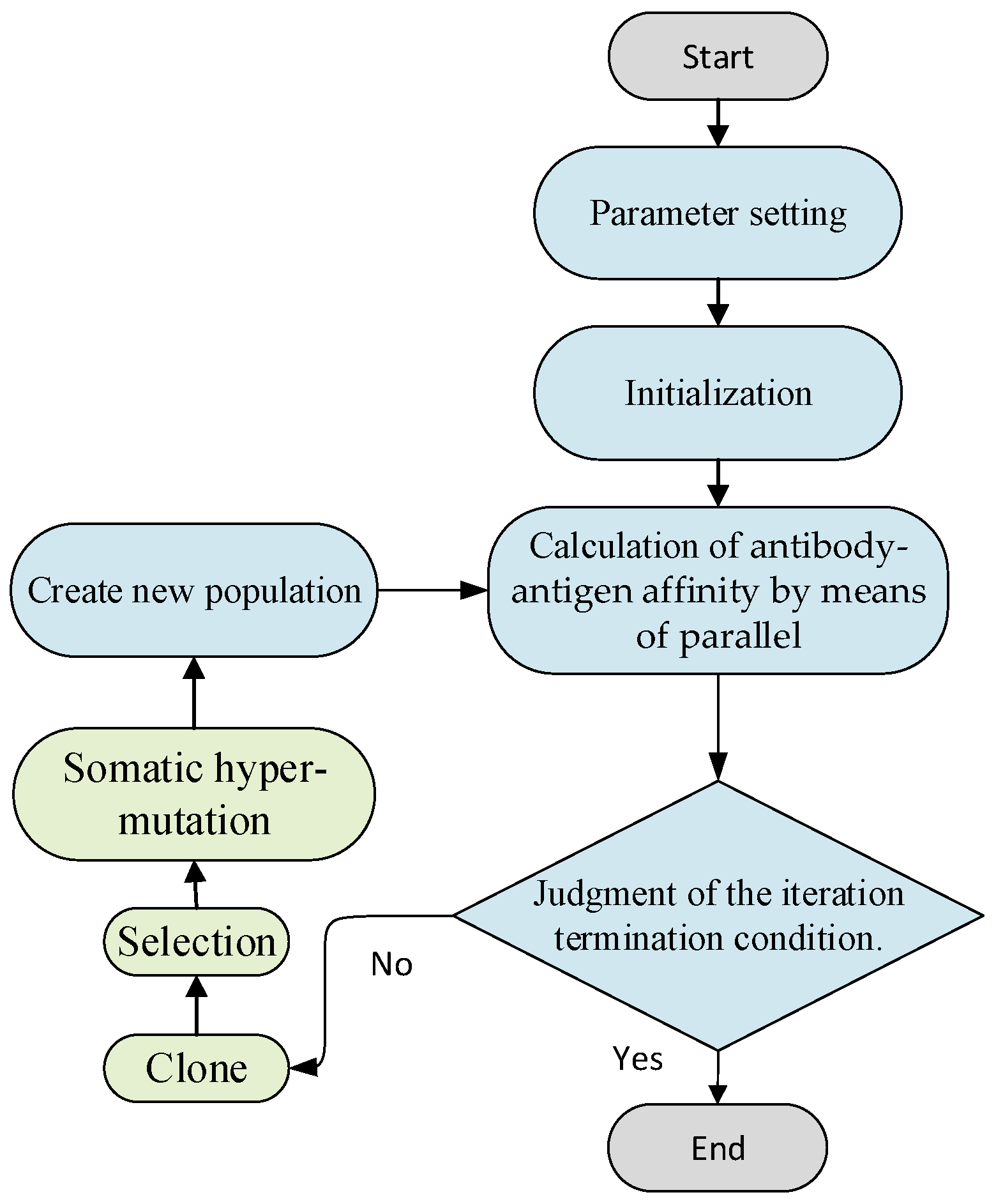
The procedure of PACSA for optimizing the SMC’s parameters is shown in Figure 9, and the steps are described in detail as follows.
Step 1. Parameter setting. Set the parameters of the PACSA, including the clone scale n m , the population number of per generation initial antibody population n p , the number of updates per generation λ , and the selection number of original antibody per generation n s .
Step 2. Initialization. The initial value of the objective function (which is the initial antibody population in this article) Y consists of Z , a binary-encoded antibody generated at random.
Step 3. Calculation of antibody–antigen affinity. In this paper, the antibody–antigen affinity is calculated according to the controller’s error integration criterion. The smaller the error integral value, the higher the antibody–antigen affinity. The error integral is calculated with the running of the simulation model. This process is the most computationally intensive part in the whole algorithm, and the error integral calculation for each simulation is independent from others. Therefore, the computing task is assigned to multiple threads of the computer for parallel computing.
Step 4. Clone. Cloning and proliferating the antibody in the antibody population Y to obtain an amplified antibody population R . Whether the antibody is cloned, as well as the number of clones, is determined by Equation (26).
Step 5. Somatic hyper-mutation. Somatic hyper-mutation of antibodies in the antibody population R to obtain R . The rate of somatic hyper-mutation is defined by Equation (25).
Step 6. Selection. Select λ high-affinity antibodies from the antibody population R to replace λ low-affinity antibodies in Y . The value of λ can be obtained from Equation (27).
Step 7. Judgment of the iteration termination condition. Whether the number of iterations meets the requirements, or whether the antibody–antigen affinity of the optimal antibody in the current population meets the requirements, and if it is satisfied, the procedure is terminated, and the result is the output. Otherwise, return to step (4).

5. Simulations Results and Analysis

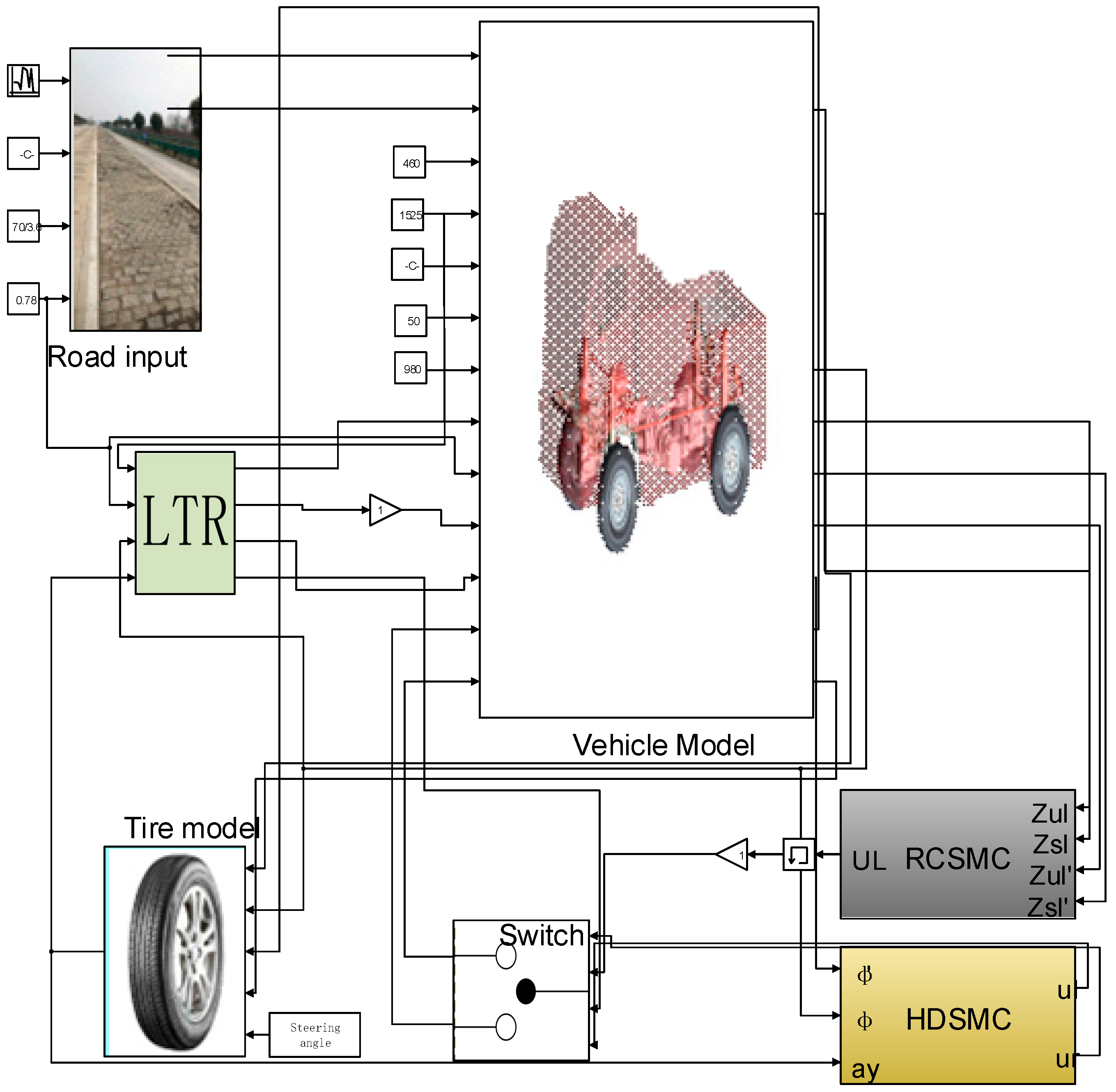
The simulation model including the 6-DOF model, the ride comfort controller, the handling stability controller, the switch strategy, and the road input models are built in MATLAB/Simulink, as shown in Figure 10. In order to verify the quality of the proposed switch control strategy, the simulations are performed under the J-turn maneuver and fishhook maneuver to evaluate the ride comfort and handling stability of the vehicle.

5.1. SMC Controller Tuning Results of PACSA

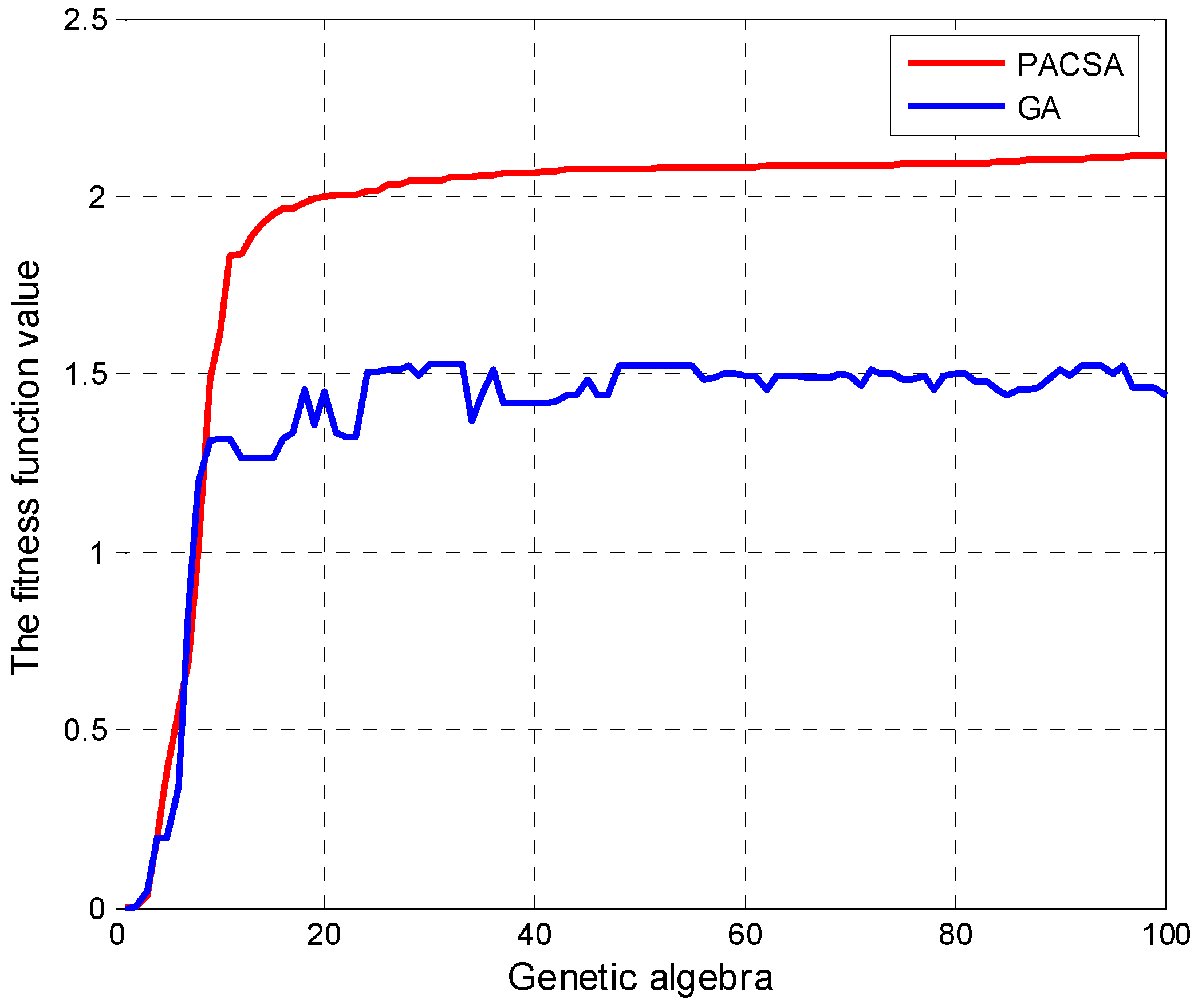
The GA-based SMC controller is designed to contrast the performance of the proposed SMC controller optimized by PACSA. The relationships between the fitness functions value and the genetic generation of GA and PACSA are shown in Figure 11.
Figure 10 displays the changes in the objective function of RCSMC and HDSMC during the PACSA tuning optimization. As can be seen from Figure 10, the changes in the objective function of RCSMC tuned by the PACSA are obvious in the first 40 generations and the corresponding convergence speed is fast. However, even until 100 generations, no convergence occurred during the GA tuning process. In addition, the whole tuning process of the GA lasted for 33 h, and the PACSA optimization procedure took only 6 h.
The optimized parameter results based on the GA and the PACSA are listed in the Table 5.
According to the optimized parameters in Table 5, the optimized RCSMC and HDSMC are obtained. Then the control of hydro-pneumatic suspension is simulated based on the two optimized controllers respectively, which reflects the optimizing ability for SMC of the PACSA and GA. The control results are obtained as follows.
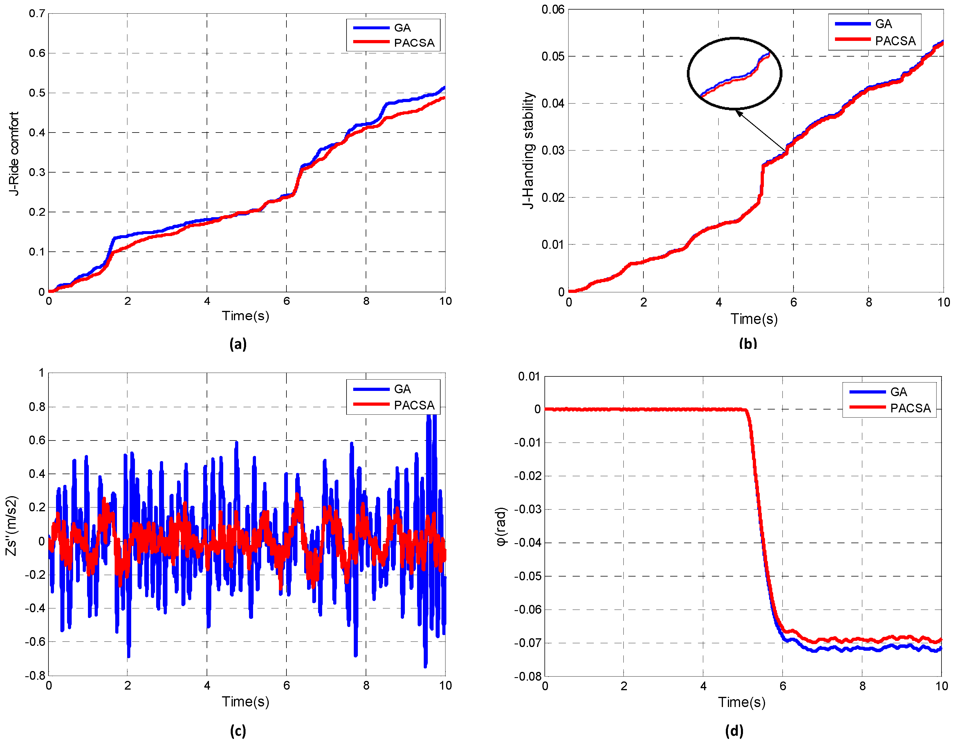
Figure 12a,b shows the dynamic responses of the objection values of the RCSMC and HDSMC. Figure 12c,d describes the dynamic responses of the vehicle vertical acceleration and the roll angle of the vehicle, respectively. Obviously, compared with the optimization results of GA, the values of the objective function, vehicle vertical acceleration, and roll angle optimized by PACSA perform better.
Above all, it can be concluded that the convergence rate, running time, and optimized results of the PACSA approach are better than the GA approach, which indicates that PACSA is more suitable for tuning the parameters of the SMC controller.

5.2. Results of Switch Control Strategy

According to the optimization results mentioned in Table 5, the RCSMC and the HDSMC are obtained. A comparison between the proposed switch control SMC (Switched SMC) and two conventional SMCs (HDSMC and RCSMC) is discussed, which can better assert that the proposed control is superior. In order to demonstrate the effectiveness of the proposed switch control strategy, different steering maneuvers including J-turn and Fishhook are tested. Furthermore, to better illustrate the adaptability of control strategy, two different typical road conditions including random road and bump road are built. The related parameters of the vehicle driving state and the corresponding road input are listed in Table 6.

5.2.1. J-Turn Maneuver

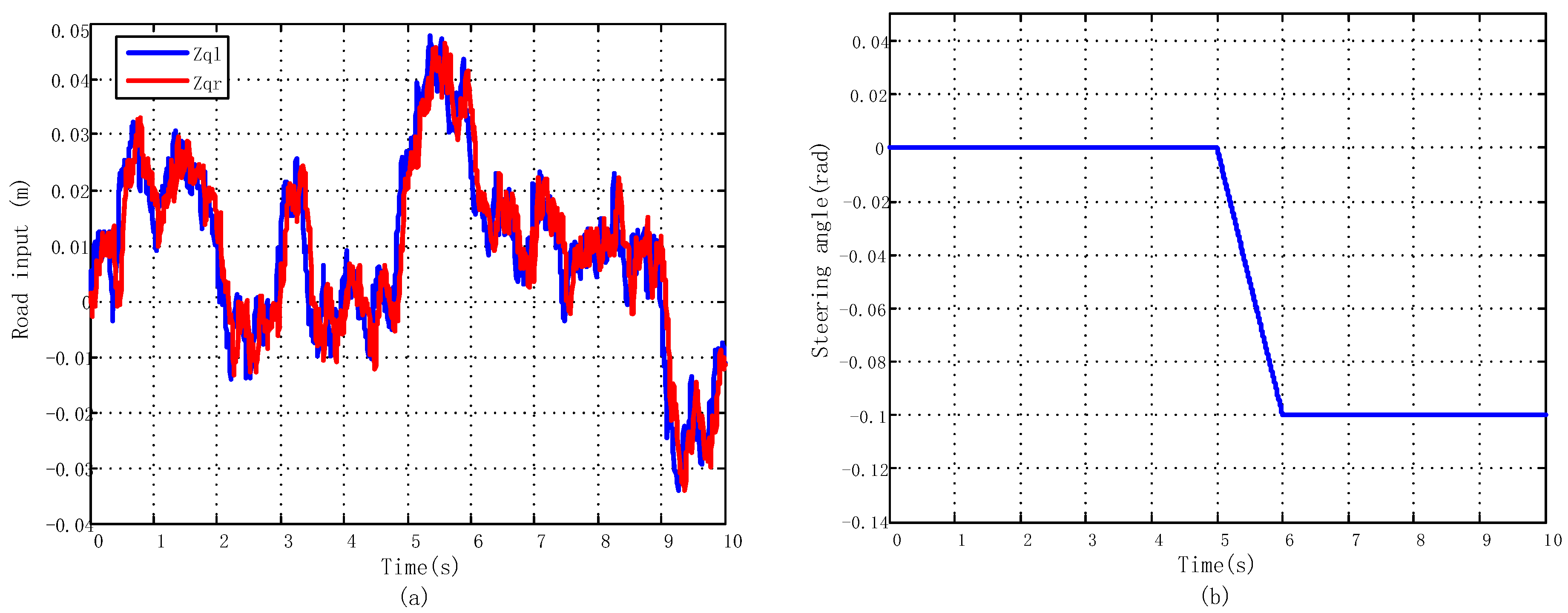
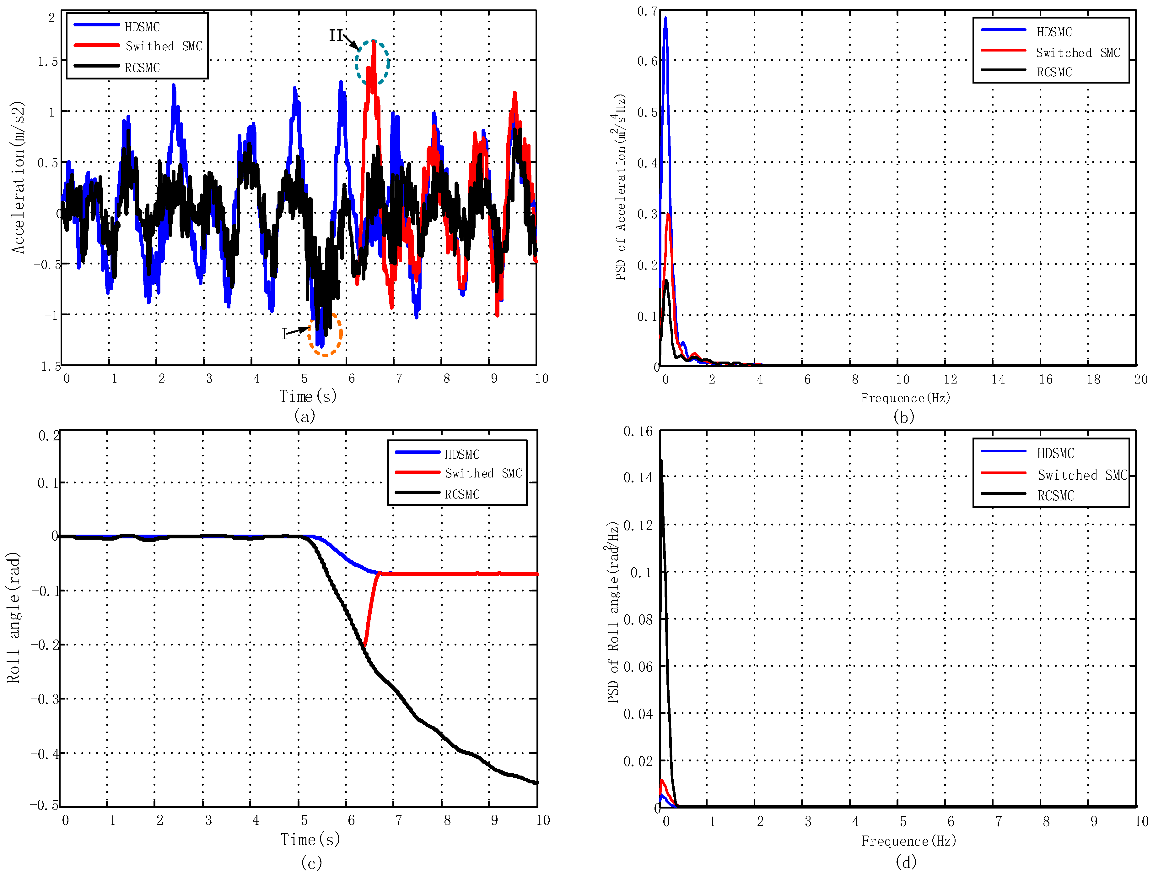
The random road input is shown in Figure 13a, and the vehicle steering angle of J-turn maneuver is displayed in Figure 13b. The dynamic responses of the HDSMC-controlled vehicle (blue lines), RCSMC-controlled vehicle (black lines), and the vehicle with the Switched SMC (red lines) are shown in Figure 14.
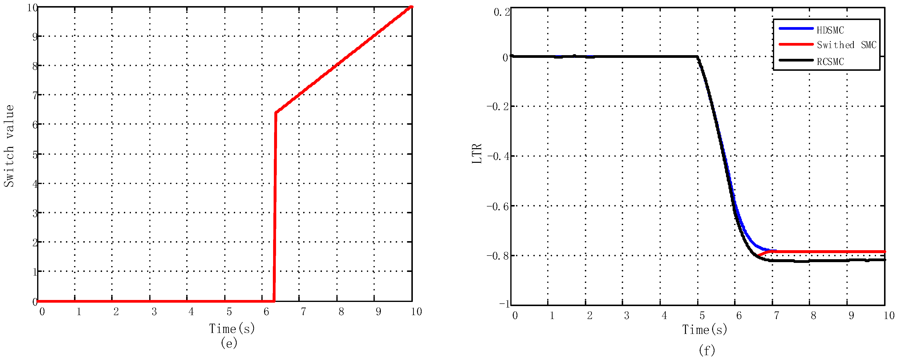
It can be seen from Figure 13b that the vehicle is going straight in the time range of [0, 5] s, and the LTR value is much smaller than the threshold. During this period, the main task for the Switched SMC is to pursue the ride comfort. Therefore, the vehicle’s vertical acceleration curves in Figure 14a during this period by the RCSMC and Switched SMC are basically identical, and the ride comfort of HDSMC is noticeably worse than that of the other two controllers. Moreover, the roll angle of the vehicle is small with different controllers during the time of [0, 5] s. The J-turn begins at the 5th second; then the vehicle roll angle and the LTR increases rapidly. The sudden steering has an impact on the ride comfort of the vehicle (point I), which is can be seen in Figure 14a. As a result, the switch of Switched SMC is not active until the LTR reaches the threshold at the 6.6th s; then the main purpose of the Switched SMC changes from the ride comfort of the vehicle to the handling stability of the vehicle. As shown in Figure 14b–f, during [6.6, 10], the values of the roll angle are reduced significantly and the LTR is dragged towards to the set value with the control of the Switched SMC. However, the LTR of the vehicle with the RCSMC is increasing with the steering of the vehicle, which is likely to cause unsafe driving conditions that lead to accidents and delays. In addition, the switch action also can be confirmed by the switch value in Figure 14e. When the switch value changes from 0 to positive, then the switch occurs. In addition, the switch action of the Switched SMC causes to a certain extent an impact on the ride comfort of the vehicle, which is point II shown in Figure 14a. The frequency domain response of the body acceleration and roll angle are shown in Figure 14c,d, which provide further obvious vindication of the Switched SMC. On the one hand, the curve in Figure 14c indicates that the Switched SMC performs better than the HDSMC with respect to ride comfort. On the other hand, curves in Figure 14d validate the superior stability of the vehicle with Switched SMC than the RCSMC. In other words, Switched SMC can take care of both sides of ride comfort and handling stability rather than one aspect.
In order to validate the robustness of the suspension system, simulations considering the uncertainty of system parameters and external disturbances were performed. In this paper, road disturbance was used as the external uncertain disturbance factor. The spring mass, vehicle speed, and suspension damping were used as the internal uncertain disturbance of the system.
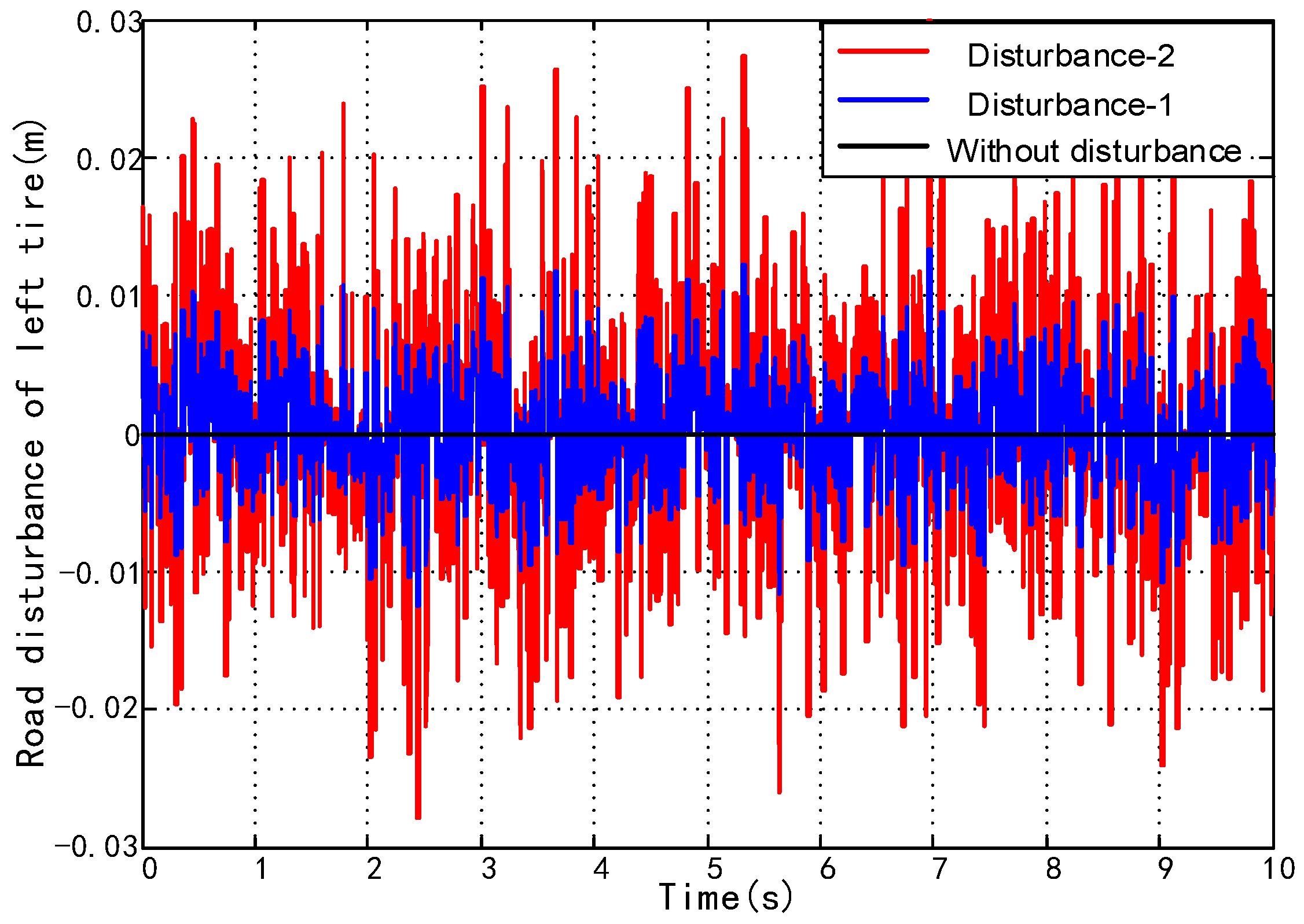
Taking the working conditions in Figure 13 as the initial conditions without disturbance, and the road disturbance signal is shown in Figure 15, which is imposed on the left tire.
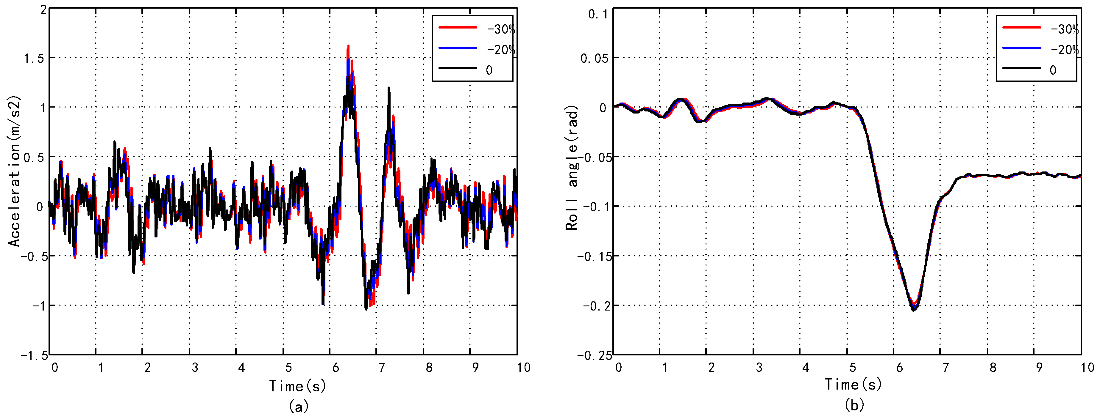
It can be seen from Figure 15, two road disturbances are imposed on the system respectively, and disturbance-2 is more serve than disturbance-1. On the one hand, the acceleration curves of the three conditions are roughly similar in the aspects of amplitude and trend in Figure 16a. On the other hand, the roll angle curves in Figure 16b show almost no difference compared with the initial system without disturbance. In other words, the ride comfort and the stability are stable, and the suspension system has excellent immunity to external disturbances.
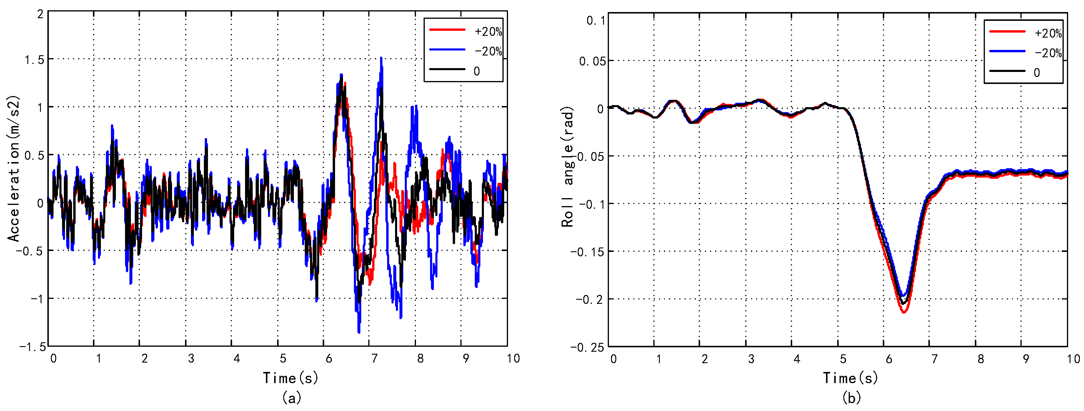
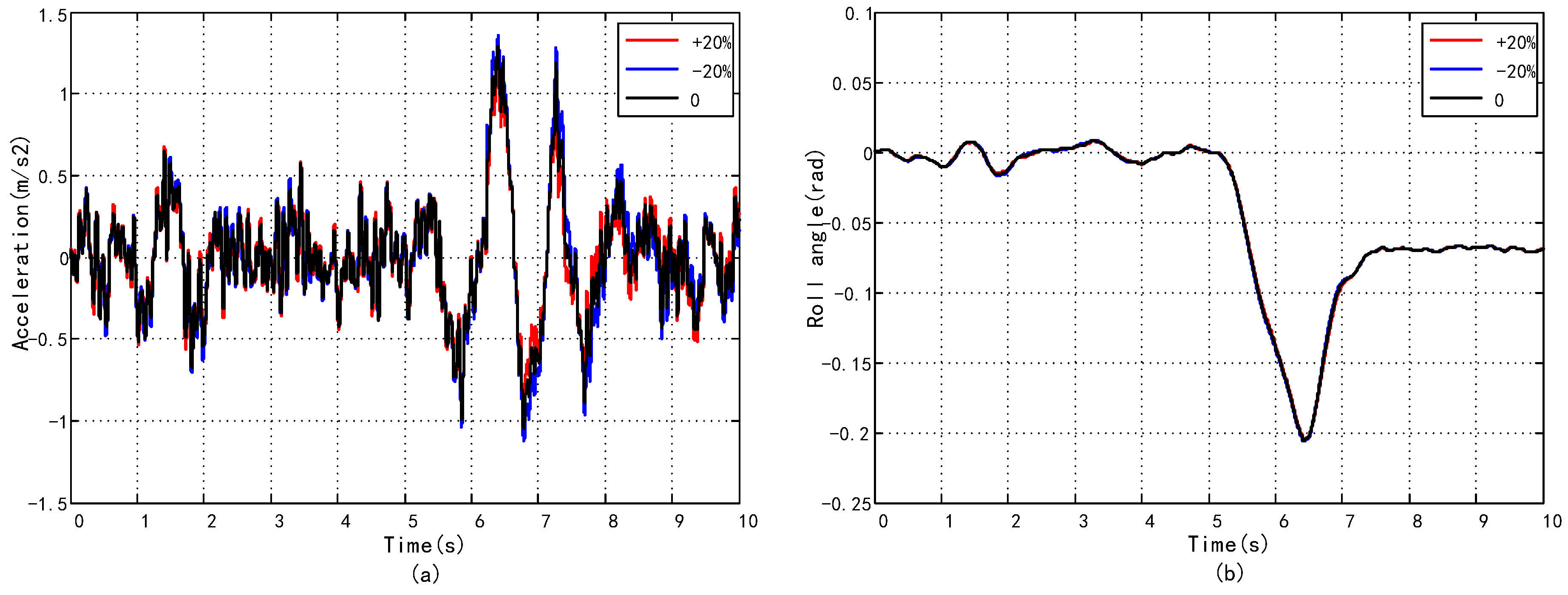
Taking into account the typical non-linear characteristics of the suspension system, the following three parameters of the suspension system, unspring mass, damping, and vehicle speed, are used as internal uncertainties to validate the system robustness. The corresponding simulation results are shown from Figure 17, Figure 18 and Figure 19.
The systems with three different unspring masses are compared in Figure 17. The black curve represents the initial condition with a sprung mass of 1525 kg, and the red and blue curves represent an increase and decrease of 20% of the sprung mass on the basis of the initial condition, respectively. As shown in Figure 16a, the differences between the three curves are small both in terms of trend and amplitude. The roll angle curves in Figure 17b show that the trends of the three conditions are basically the same, and the amplitude is slightly different.
As shown in Figure 18, the red and blue curves represent an increase and decrease of 20% of the damping comparing to the black curve of the initial condition, respectively. Obviously, changes in suspension damping in this range have almost no effect on the acceleration and roll angle of the vehicle system. As a result, the suspension system in this paper has a good anti-interference ability to the parameter uncertainty of suspension damping.
Figure 19 shows the impact of vehicle speed changes on the suspension system. The vehicle speed under the initial condition is 70 km/h, which is the maximum speed of the rescue vehicle in this paper. Therefore, reducing vehicle speed by 20% and 30%, respectively, was used to verify the interference caused by the uncertainties of vehicle speed on the system. As can be seen from the two diagrams in Figure 19, the system has a strong anti-interference ability to vehicle speed uncertainty.
As a result, it can be seen from the above simulation results and analysis that the suspension system has strong ability to resist the disturbances, which were caused by both the external uncertainty and parametric uncertainty. In other words, the suspension system of the rescue vehicle built in this paper has good stability and robustness.
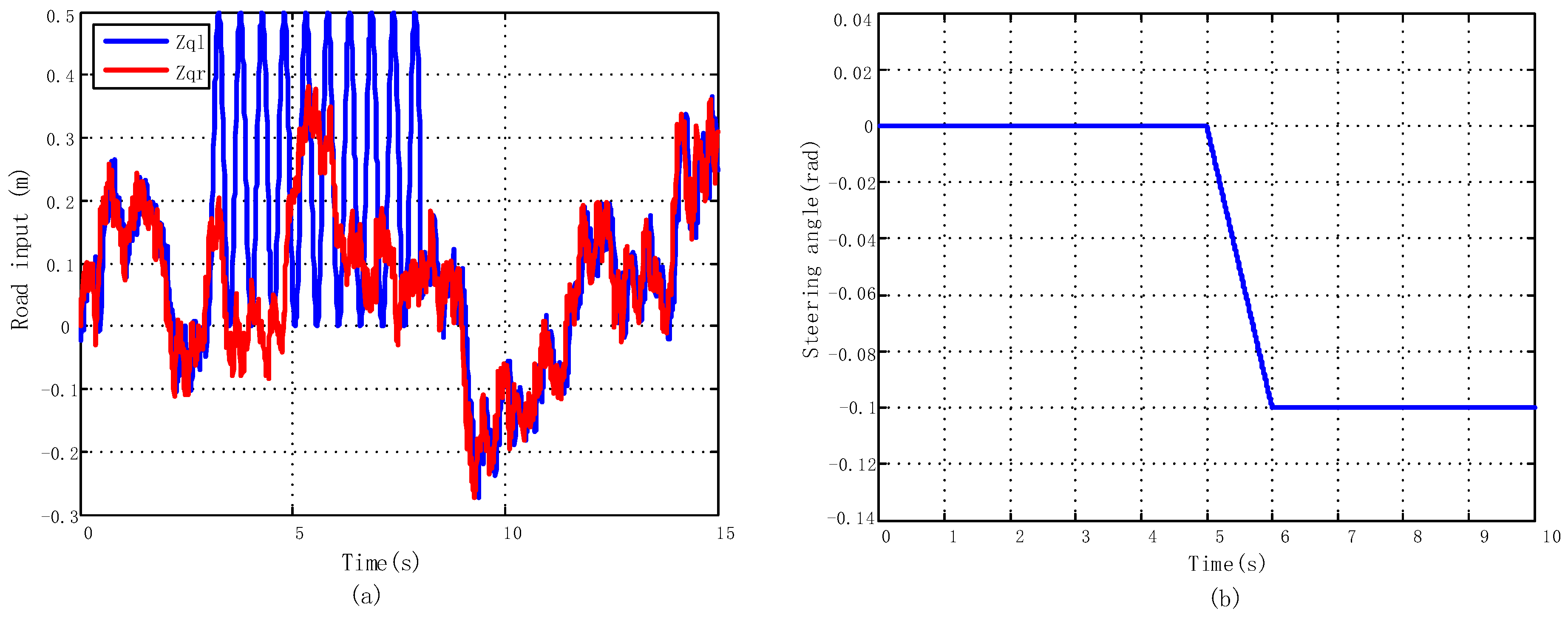
In addition, in order to better illustrate the adaptability of the proposed switch control strategy, a bumpy road was used as the road input, which is shown in Figure 20a, and the vehicle steering angle of the J-turn maneuver is displayed in Figure 20b. The dynamic responses of the HDSMC-controlled vehicle (blue lines), RCSMC-controlled vehicle (black lines), and the vehicle with the Switched SMC (red lines) are shown in Figure 21.
The results for the bump road in Figure 21 are similar to those of Figure 14. In the time range of [0, 3] s, the vehicle vertical acceleration of the suspension system with RCSMC is significantly smaller than HDSMC and Switched SMC. The vehicle vertical acceleration and roll angle become bigger after 3 s because of the input of bump road; however, the vertical acceleration of the suspension system with RCSMC is still smaller than the vehicles with the other two controllers during the time of [3, 6.5] s. One can notice that at time 6.5 s, when the Switched SMC is switched, the performance of roll angle and LTR is better than the RCSMC-controlled vehicle. Consequently, the value of LTR is stabilized to its set value with the control of Switched SMC, whereas the value changes in an unsafe range with RCSMC. Similarly, there are also shocks that are induced by the switch action of the vehicle, which are not obvious as in Figure 14a because of the worse road condition. The frequency domain response of the body acceleration and roll angle are shown in Figure 21c,d, which provide further obvious vindication of the Switched SMC. It can also be seen that the Switched SMC can take care of both sides of ride comfort and handling stability rather than one aspect.

5.2.2. Fishhook Maneuver

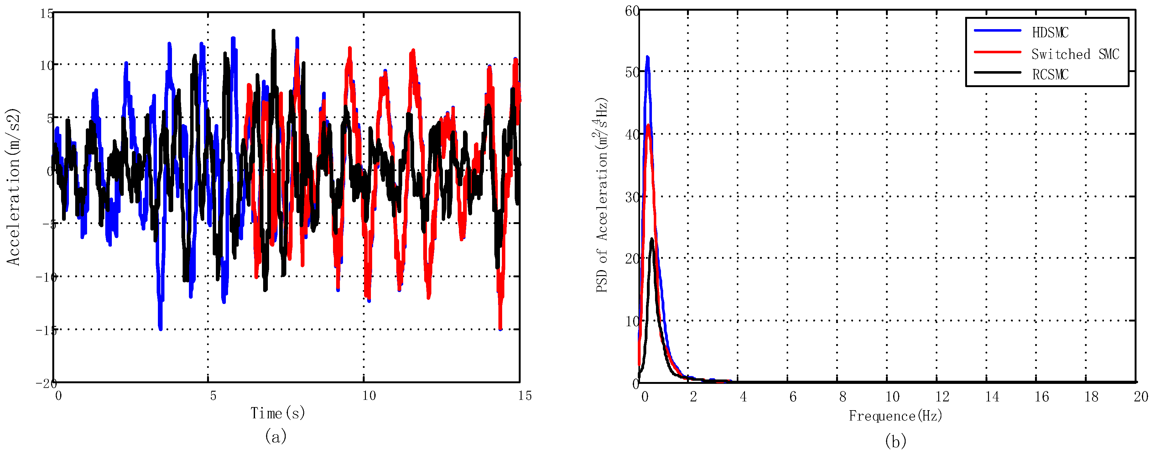
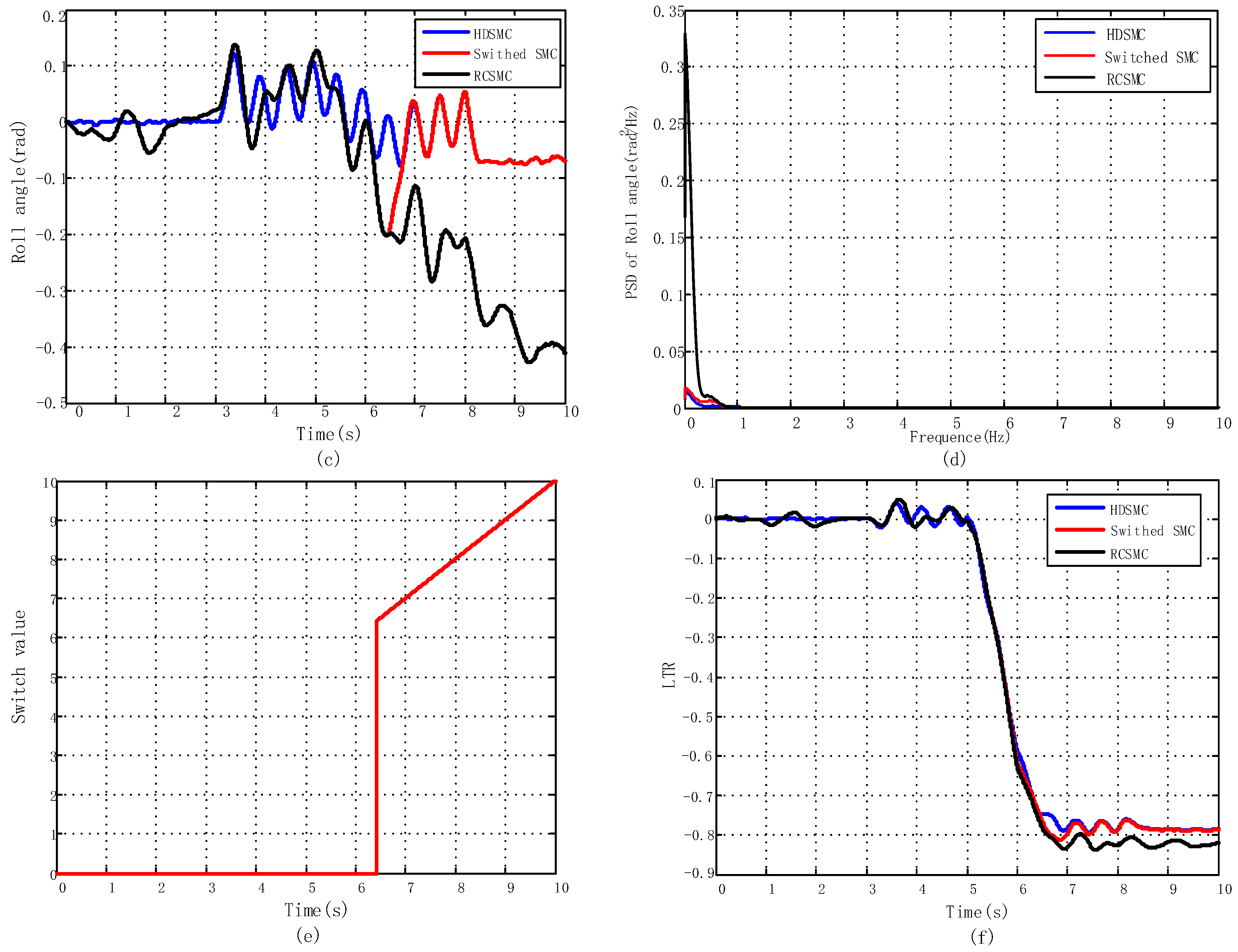
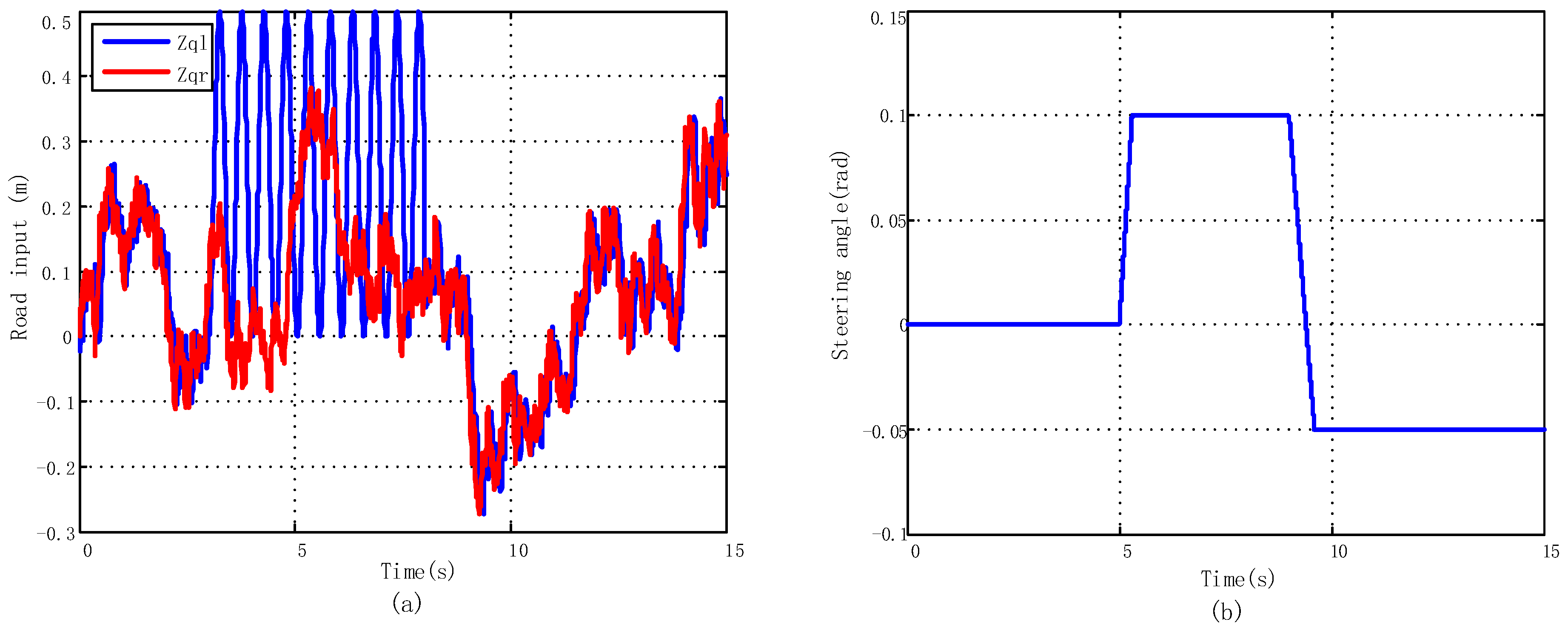
The fishhook maneuver is applied to demonstrate the proposed switch control strategy of the hydro-pneumatic suspension, and the vehicle steering angle under the fishhook maneuver is shown in Figure 22b. The random road shown in Figure 21a and the bump road displayed in Figure 23a are used as the road input of simulation, respectively.
The dynamic responses of the HDSMC-controlled vehicle (blue lines), RCSMC-controlled vehicle (black lines), and the vehicle with the Switched SMC (red lines) are shown in Figure 23.
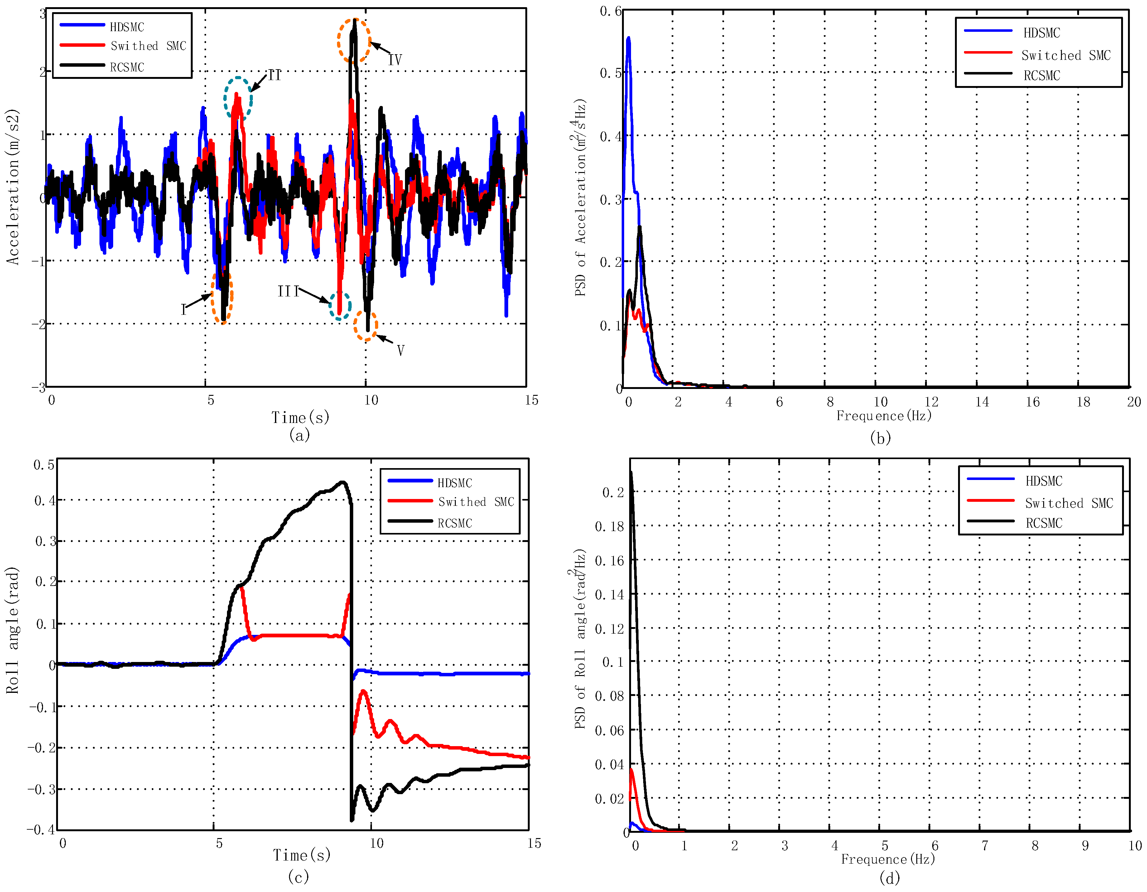
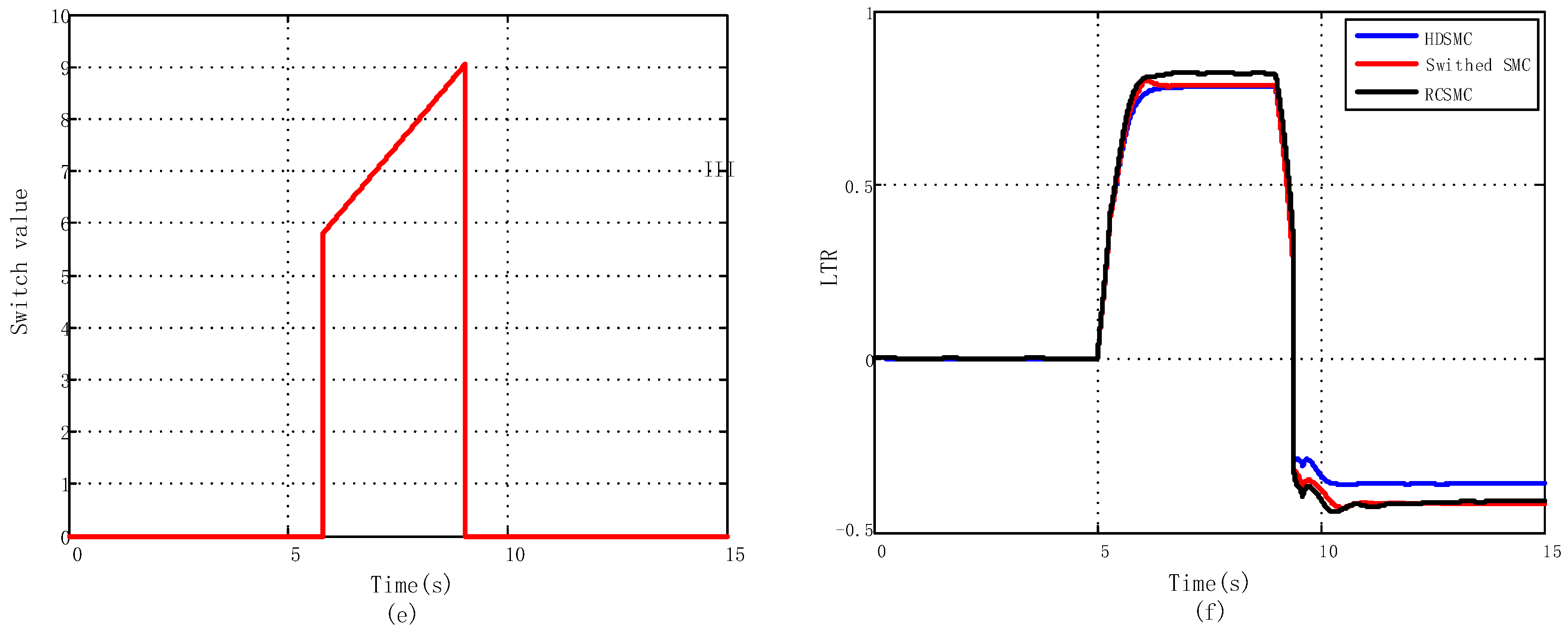
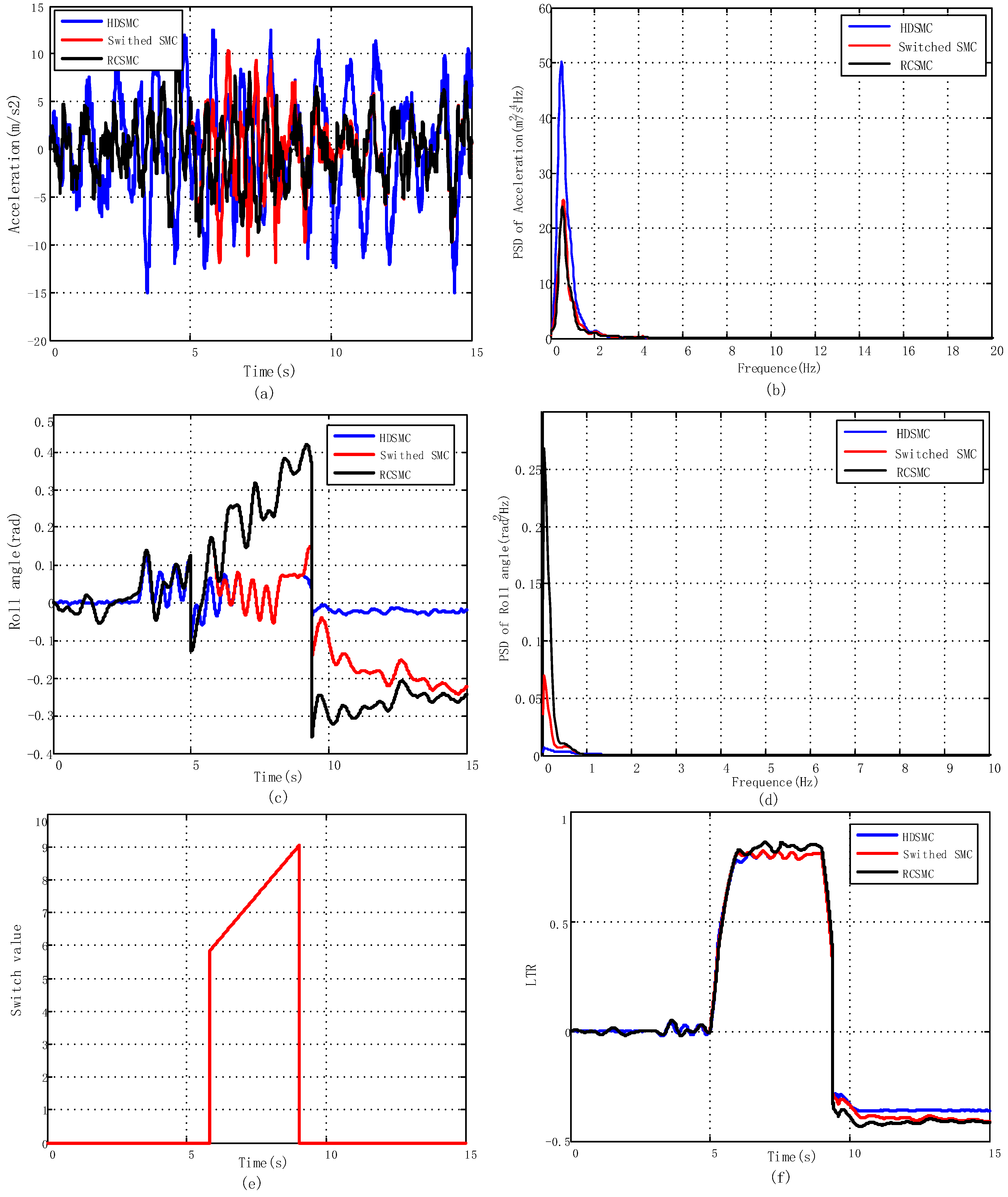
Once the fishhook steering maneuver is exerted at the 5th second in Figure 22b, the value of LTR goes up rapidly and reaches 0.8 at the 5.8th s, and then the controller is switched to drag the LTR to the set value. Until the 9th s, the value of LTR is reduced to less than the set value. Then the controller is switched to pursue the ride comfort of the vehicle. The switch actions are obvious, which can be observed and proved in Figure 23e. The steering angle changes rapidly in the opposite direction in the time rage of [9 9.4] s, but the value of LTR does not rise to the set value, and the control mode does not switch. It is easy to see that the roll angle and the LTR of the vehicle with the Switched SMC become bad and move toward the value of the RCSMC-controlled vehicle, because the Switched SMC has been pursuing the ride comfort when the vehicle is not in danger from the 9th s. The mutation points II and III in Figure 23a are caused by the switch action, and the mutation points I, IV, and V are induced by the steering actions. From the frequency domain response of curves shown in Figure 23c,d, the same conclusion can be reached that the Switched SMC can simultaneously improve the ride comfort and handling stability under this condition compared with the conventional SMC controlled suspension.
The rescue vehicle dynamic responses based on the switch strategy under the bump road and the fishhook maneuver (Figure 24) are shown in Figure 25. Similarly, the analysis results are the same as those in Figure 23, and the switch actions of the Switched SMC come true according to LTR value.
Based on the analysis of simulation results mentioned above, it is concluded that (1) the PACSA performs better than GA in terms of the parameters optimization of the SMC; (2) the switch strategy proposed in this paper is all effective under different vehicle speeds, road inputs, and the steering modes.

6. Conclusions

This paper presents a sliding mode switch control strategy for both the ride comfort and handling stability of the adjustable hydro-pneumatic suspension system of a rescue vehicle. The switch index of the Switched SMC is defined according to the value of LTR. Three different SMC controllers are designed respectively and tested through the simulations of the half-car model based on MATLAB/Simulink. AHP is applied to calculate the weight coefficients of the objective functions, and the parameters of the controller are tuned by PACSA, the optimization ability of which proved better than that of GA. The performance of the switch strategy is proved through simulations with different road input (random road and bump road), different vehicle speeds, and different steering maneuvers (J-turn steering and Fishhook steering).
Compared with the conventional SMC controlled hydro-pneumatic suspension system, the simulation results show that the proposed switch control strategy has the following advantages:
(1)
The PACSA performs better than a genetic algorithm in terms of parameter optimization of the SMC.
(2)
The proposed switch control strategy can simultaneously address concerns on both ride comfort and handling stability under different road surfaces and driving conditions through switch actions.
In the future work, on the one hand, it is essential to reduce the shocks induced by the switch action, which will make the switch control strategy work better. On the other hand, we will apply the proposed control strategy based on related algorithms to a real fire rescue prototype to validate the proposed strategy when the prototype is completed in the future.

Author Contributions

conceptualization, C.Z. and X.L.; methodology, F.X., C.Z. and W.C.; software, C.Z.; validation, F.X., C.Z. and W.C.; writing—original draft preparation, C.Z.; writing—review and editing, C.Z. and F.X.; visualization, C.Z.; supervision, W.C.; project administration, C.Z. and X.L.; funding acquisition, X.L. All authors have read and agreed to the published version of the manuscript.

Funding

This research was funded by The National Key Research and Development Program of China under Grant No. 2016YFC0802900.

Data Availability Statement

The data used to support the findings of this study are available from the corresponding author upon request.

Conflicts of Interest

The authors declare no conflict of interest.

References

  1. Hongbin, R.; Lin, Y. Sliding mode control based on improved virtual reference model for damping adjustable hydro-pneumatic suspension systems. J. Vibroeng. 2015, 17, 3196–3210. [Google Scholar]
  2. Chen, Z.; Liu, X. Optimal Sliding Mode Control for an Active Suspension System Based on a Genetic Algorithm. Algorithms 2018, 11, 205. [Google Scholar]
  3. Riofrio, A.; Sanz, S.; Boada, M.J.L. A LQR-Based Controller with Estimation of Road Bank for Improving Vehicle Lateral and Rollover Stability via Active Suspension. Sensors 2017, 17, 2318. [Google Scholar] [CrossRef] [PubMed] [Green Version]
  4. Wang, S.; Lu, Z.; Liu, X. Active control of hydro pneumatic suspension parameters of wheel loaders based on road condition identification. Int. J. Adv. Robot. Syst. 2018, 15. [Google Scholar] [CrossRef]
  5. Awad, M.N.; Sokar, M.I. Hydro-Pneumatic Energy Harvesting Suspension System Using a PSO Based PID Controller. SAE Int. J. Commer. Veh. 2018, 11, 1–11. [Google Scholar] [CrossRef]
  6. Pradhan, S.; Singh, B. A Composite Sliding Mode Controller for Wind Power Extraction in Remotely Located Solar PV-Wind Hybrid System. IEEE Trans. Ind. Electron. 2019, 66, 5321–5331. [Google Scholar] [CrossRef]
  7. Biricik, S.; Komurcugil, H. Protection of Sensitive Loads Using Sliding Mode Controlled Three-Phase DVR with Adaptive Notch Filter. IEEE Trans. Ind. Electron. 2019, 66, 5465–5475. [Google Scholar] [CrossRef]
  8. Farahmandrad, M.; Ganjefar, S. Fuzzy Sliding Mode Controller Design for a Cooperative Robotic System with Uncertainty for Handling an Object. J. Dyn. Syst. Meas. Control Trans. ASME 2019, 141. [Google Scholar] [CrossRef]
  9. Abtahi, S.M. Suppression of chaotic vibrations in suspension system of vehicle dynamics using chattering-free optimal sliding mode control. J. Braz. Soc. Mech. Sci. Eng. 2019, 41, 210. [Google Scholar] [CrossRef]
  10. Soltanpour, M.R.; Khooban, M.H. A particle swarm optimization approach for fuzzy sliding mode control for tracking the robot manipulator. Nonlinear Dyn. 2013, 74, 467–478. [Google Scholar] [CrossRef]
  11. Long, Y.; Du, Z.-j. Robust Sliding Mode Control Based on GA Optimization and CMAC Compensation for Lower Limb Exoskeleton. Appl. Bionics Biomech. 2016, 2016, 5017381. [Google Scholar] [CrossRef] [PubMed] [Green Version]
  12. Li, Z.; Xia, Y.; Sahli, H. CSA-DE/EDA: A Clonal Selection Algorithm Using Differential Evolution and Estimation of Distribution Algorithm. In Proceedings of the Advances in Brain Inspired Cognitive Systems, 9th International Conference, Xi’an, China, 7–8 July 2018. [Google Scholar]
  13. Hashemipour, M.S.; Soleimani, S.A. Artificial immune system based on adaptive clonal selection for feature selection and parameters optimization of support vector machines. Connect. Sci. 2016, 28, 47–62. [Google Scholar] [CrossRef]
  14. Liang, H.; Kang, F. Adaptive chaos parallel clonal selection algorithm for objective optimization in WTA application. OPTIK 2016, 127, 3459–3465. [Google Scholar]
  15. Srinivasa Rao, B.; Vaisakh, K. Multi-objective adaptive Clonal selection algorithm for solving environmental/economic dispatch and OPF problems with load uncertainty. Int. J. Electr. Power Energy Syst. 2013, 53, 390–408. [Google Scholar] [CrossRef]
  16. Tan, D.; Wang, H. Fully Homomorphic Encryption Based On the Parallel Computing. Ksii Trans. Internet Inf. Syst. 2018, 12, 497–522. [Google Scholar]
  17. Liang, B.; Zheng, S. The attribute reduction algorithm based on parallel computing. J. Intell. Fuzzy Syst. 2017, 32, 1867–1875. [Google Scholar] [CrossRef]
  18. Yuan, Z. Research on the Steady-State Model of Tire; Jilin University: Changchun, China, 2006. [Google Scholar]
  19. Kasprzak, E.M. Extension of the Nondimensional Tire Theory to General Operating Conditions; State University of New York at Buffalo: Buffalo, NY, USA, 2007. [Google Scholar]
  20. Wei, Y.; Feng, X.; Zhang, F.Q. State of the art for tire dynamical model research. J. Automot. Saf. Energy 2014, 5, 311–323. [Google Scholar]
  21. Yasheen, B. Large Tyre Testing and Modelling for Handling; University of Pretoria: Pretoria, South Africa, 2015. [Google Scholar]
  22. Iraj, D.; Ali, A.R. Identification of tire forces using Dual Unscented Kalman Filter algorithm. Nonlinear Dyn. 2014, 78, 1907–1919. [Google Scholar]
  23. Zhang, L. Analysis and Control of Non-stationary Ride Comfort of Vehicles with Random Excitation; Northeastern University: ShenYang, China, 2012. [Google Scholar]
  24. Cheng, L.; Wei, L. Neutral network-PID control algorithm for semi-active suspensions with magneto-rheological damper. IEEE Sens. J. 2015, 18, 4432–4444. [Google Scholar]
  25. Li, H.; Zhao, Y. Design of an improved predictive LTR for rollover warning systems. J. Braz. Soc. Mech. Sci. Eng. 2017, 39, 3779–3791. [Google Scholar] [CrossRef]
  26. Huangfu, Y.; Zhuo, S. Robust Voltage Control of Floating Interleaved Boost Converter for Fuel Cell Systems. IEEE Trans. Ind. Appl. 2018, 54, 665–674. [Google Scholar] [CrossRef]
  27. Nagarkar, M.P.; Patil, G.; Vikhe, J. Optimization of nonlinear quarter car suspension-seat-driver model. J. Adv. Res. 2016, 7, 991–1007. [Google Scholar] [CrossRef] [PubMed] [Green Version]
  28. Liu, J. Simulation of Sliding Mode Control Based on MATLAB; Tsinghua University press: Beijing, China, 2015; pp. 4–25. [Google Scholar]
  29. Susatio, Y.; Oktaviana, L. Design of half-car active suspension system for passenger riding comfort. J. Phys. Conf. Ser. 2018, 1075, 012030. [Google Scholar] [CrossRef]
  30. Faried, H.; Waleed, F.F. Ride comfort performance of a vehicle using active suspension system with active disturbance rejection control. Int. J. Veh. Noise Vib. 2015, 11, 78–101. [Google Scholar]
  31. Zhang, L.; Li, L. Rollover prevention control for a four in-wheel motors drive electric vehicle on an uneven road. Sci. China Technol. Sci. 2018, 61, 934–948. [Google Scholar] [CrossRef]
  32. Liao, C.; Wu, X. Semi-active Suspension Anti Rollover Control for Bus Using Fuzzy Sliding Mode Theory. J. Xiamen Univ. 2014, 3, 373–377. [Google Scholar]
  33. Dnyandeo, D.S.; Ramjee, P. Application of AHP for Ranking of Total Productive Maintenance Pillars. Wirel. Pers. Commun. 2018, 100, 449–462. [Google Scholar]
  34. De Castro, L.N.; Von Zuben, F.J. Learning and optimization using the clonal selection principle. Ieee Trans. Evol. Comput. 2002, 6, 239–251. [Google Scholar] [CrossRef]
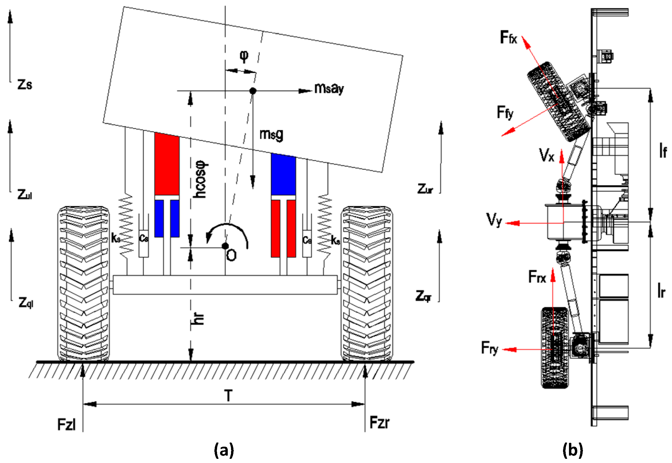
Figure 1. Schematic of a six-degrees-of-freedom (6-DOF) rescue vehicle model: (a) the 4-DOF roll motion model; (b) the 2-DOF steer-yaw model.
Applsci 10 01852 g001
Figure 2. Steering angle of tires in the Pacejka tire simulation.
Applsci 10 01852 g002
Figure 3. Simulation results of Pacejka tires: (a) Slide slip angle; (b) Yaw velocity; (c) Lateral acceleration; (d) Lateral force.
Applsci 10 01852 g003
Figure 4. Simulated displacement curves of the left and right tires.
Applsci 10 01852 g004
Figure 5. Sliding mode switch control strategy of adjustable hydro-pneumatic suspension.
Applsci 10 01852 g005
Figure 6. Dynamic switch control block diagram of the hydro-pneumatic suspension system.
Applsci 10 01852 g006
Figure 7. Weight coefficients evaluation process based on analytic hierarchy process (AHP).
Applsci 10 01852 g007
Figure 8. Hierarchical analysis model of AHP.
Applsci 10 01852 g008
Figure 9. Process of the parallel adaptive clonal selection algorithm (PACSA).
Applsci 10 01852 g009
Figure 10. Vehicle model in MATLAB/Simulink.
Applsci 10 01852 g010
Figure 11. The relationships between the fitness functions value and the genetic generation of GAand PACSA.
Applsci 10 01852 g011
Figure 12. SMC control comparison optimized by PACSA and GA: (a) the objective function of ride comfort; (b) the objective function of handling stability; (c) the body vertical acceleration; (d) the roll angle.
Applsci 10 01852 g012
Figure 13. The input signals of vehicle: (a) the random road; (b) the steering angle under J-turn maneuver.
Applsci 10 01852 g013
Figure 14. The rescue vehicle dynamic response based on the switch strategy under the random road and the J-turn maneuver: (a) the vehicle body vertical acceleration in time domain; (b) the roll angle acceleration in time domain; (c) the vehicle body vertical acceleration in time domain and in frequency domain; (d) the roll angle acceleration in frequency domain; (e) the switch value; (f) the load transfer ratio (LTR).
Applsci 10 01852 g014aApplsci 10 01852 g014b
Figure 15. The road disturbance imposed on the system.
Applsci 10 01852 g015
Figure 16. The robustness simulation curves with the road disturbance: (a) the vehicle body vertical acceleration in time domain; (b) the roll angle acceleration in time domain.
Applsci 10 01852 g016
Figure 17. The robustness simulation curves with uncertainty of unspring mass: (a) the vehicle body vertical acceleration in time domain; (b) the roll angle acceleration in time domain.
Applsci 10 01852 g017
Figure 18. The robustness simulation curves with the uncertainty of suspension damping: (a) the vehicle body vertical acceleration in time domain; (b) the roll angle acceleration in time domain.
Applsci 10 01852 g018
Figure 19. The robustness simulation curves with the uncertainty of vehicle speed: (a) the vehicle body vertical acceleration in time domain; (b) the roll angle acceleration in time domain.
Applsci 10 01852 g019
Figure 20. The input signals of vehicle: (a) the bump road; (b) the steering angle under J-turn maneuver.
Applsci 10 01852 g020
Figure 21. The rescue vehicle dynamic response based on the switch strategy under the bump road condition and the J-turn maneuver: (a) the vehicle body vertical acceleration in time domain; (b) the roll angle acceleration in time domain; (c) the vehicle body vertical acceleration in time domain in frequency domain; (d) the roll angle acceleration in frequency domain; (e) the switch value; (f) the LTR.
Applsci 10 01852 g021aApplsci 10 01852 g021b
Figure 22. The input signals of vehicle: (a) the random road; (b) the steering angle under the fishhook maneuver.
Applsci 10 01852 g022
Figure 23. The rescue vehicle dynamic response based on the switch strategy under the bump road and the fishhook maneuver: (a) the vehicle body vertical acceleration in time domain; (b) the roll angle acceleration in time domain; (c) the vehicle body vertical acceleration in time domain in frequency domain; (d) the roll angle acceleration in frequency domain; (e) the switch value; (f) the LTR.
Applsci 10 01852 g023aApplsci 10 01852 g023b
Figure 24. The input signals of vehicle: (a) the bump road; (b) the steering angle under the fishhook maneuver.
Applsci 10 01852 g024
Figure 25. The rescue vehicle dynamic response based on the switch strategy under the bump road and the fishhook maneuver: (a) the vehicle body vertical acceleration in time domain; (b) the roll angle acceleration in time domain; (c) the vehicle body vertical acceleration in time domain in frequency domain; (d) the roll angle acceleration in frequency domain; (e) the switch value; (f) the LTR.
Applsci 10 01852 g025
Table 1. The parameters of the rescue vehicle’s suspension system.
Parameters SymbolValueUnit
Spring mass m s 1525 kg
Unspring mass m u 50 kg
Tread T 1.56 m
Suspension spring fitting stiffness k s 35,000 N m / rad
Suspension spring fitting damping C s 980 N m s / rad
Tire vertical elastic stiffness k t 190,000 N m / rad
Yaw moment of inertia I r 2500 kg · m 2
Roll moment of inertia I x 460 kg · m 2
Distance from the center of gravity to the center of the roll h 0.45 m
Distance from the center of gravity to the ground h r 0.5 m
Distance between the center of gravity and the front axle l f 1.27 m
Distance between the center of gravity and the rear axle l r 1.94 m
Table 2. Quantized scale factor values table.
RMS σ z ¨ s
0.92
σ φ ¨
1.18
σ z s l z u l
0.032
σ z s r z u r
0.0008
σ z u l z q l
0.00214
σ z u r z q r
0.0096
Quantized ScaleFactor γ 1
1
γ 2
0.6
γ 3
826.56
γ 4
13,225
γ 5
184,819.64
γ 6
9184.03
Table 3. Reference criterion (RI) values.
r12345678
RI000.580.91.121.241.321.41
Table 4. Weight coefficients of the controllers.
Weight Coefficients τ 1 τ 2 τ 3 τ 4 τ 5 τ 6
Handling Stability Control0.0530.86230.23620.17642.1421.661
Ride Comfort Control0.480.06131.32100009777485.8
Table 5. Optimized parameters of the PACSA and GA.
RCSMCHDSMC
PACSAGA PACSAGA
n 1 −0.575−2.55 ρ 54.73
n 2 0.65599.7 μ 32.99
n 3 0−0.063 η 2524.92
η 1114.939 κ 1 0.00120.73
μ 0.00050.15 κ 2 0.00140.0025
ζ 0.4440.39
Table 6. The related parameter settings of different conditions.
J-turn/Fishhook
Road ConditionRandom RoadBump Road
Vehicle speed70 km/h60 km/h
Road level (ISO/DIS8608)CF
G q ( n 0 ) 256 × 10 6 m 3 16,380 × 10 6 m 3
Steering angle 0 . 1 rad / ± 0 . 1 rad 0 . 1 rad / ± 0 . 1 rad
φ max 0 . 2 rad 0 . 2 rad
κ 1 0.10.1
κ 2 0.10.1