Monitoring of Namibian Encroacher Bush Using Computer Vision

Abstract

In Namibia, the encroachment by a native, but invasive bush on Savannah land leads to both environmental and economic loss. This invasive bush is, however, suitable for harvesting as a source of biomass for local industry. Harvesting biomass from the invasive bush has been shown to restore biodiversity, improve water conservation efforts, and restore grazing lands. Beyond the environmental benefits of removing the invasive bush, the raw biomass harvested is amenable to simple value-added production. Although some efforts are underway to make use of harvested biomass, current harvesting practices are not selective enough to meet governmental requirements intended to protect several species of local fauna and flora. Limitations, such as a lack of knowledge, during the harvesting process, can be overcome to a significant degree through the introduction of a smart application. This can integrate geographical context with computer vision to provide a ground-level tool for the identification of areas suitable for harvesting. This study shows that this tool can identify indigenous taxonomies with an accuracy of 76%.

1. Introduction

Namibia is an arid and water-scarce region subject to the undesired aggressive growth of invasive bush species. This research identifies the economic and environmental benefits of harvesting encroacher bush and the technological readiness level of a proposed method for providing ground-level resources for identification of suitable areas to harvest, based on currently available computer vision and Machine learning (ML) resources. Computer vision is used in this context as employees lack the ability to distinguish between bush and tree species. A techno-economic analysis is conducted, which further identifies the need for computer vision in the Namibian agricultural environment. Computer vision is comprised of the identification of image patterns. This is accomplished with the use of ML. Inevitably, data need to be collected and a suitable ML algorithm trained, such that a digital monitoring tool can be created. The central goal of this tool is to answer the question: Can the Namibian encroacher bush be monitored with established technologies, to both benefit the economic and ecological environment?

There are various plant identification projects focusing on leaves [1] and fruit [2]. During the literature study, no research was identified that utilized encroacher bush and full plant images as the identification database. This describes the novelty of this research.

A literature review of the technological state of plant identification algorithms, using computer vision, was given by [3]. The aim of these projects was classifying plants through close-up images of leaves, flowers, or bark. These photographs were low-noise photos, as they only displayed the object of interest within a uniform background. In the work conducted by [3], only one team competing in the ImageCLEFcampaign used the entire plant for classification, namely the team of Pl@ntNet. ImageCLEF’s aim is “to support the advancement of the field of visual media analysis, indexing, classification, and retrieval, by developing the necessary infrastructure for the evaluation of visual information retrieval systems operating in both monolingual, cross–language and language-independent contexts” [4]. Pl@ntNet has also developed an application and website, where users can upload their photos of various plant organs, such as bark, leaves, flower, and fruit, or the entire plant [5]. Their algorithm classifies the input images according to the established database. Key findings are that there is also a lack of data, and a large number of images still have to be collected to cover all 220,000 plant species. Usually, these studies are conducted with images containing neutral and homogeneous backgrounds, to simplify the problem. Furthermore, the study concludes that plant identification is usually based on leaves or single plant organs. For feature extraction from the images, the organ shapes are the most prevalent features used. However, identification accuracy was increased in studies where multiple features were used.

Similar challenges, as experienced during the bush monitoring process, were described by [6]. Firstly, the problems associated with existing datasets are described. The relevant problems in the context of the project include that databases suffer from mislabeled pictures because it is difficult for non-botanists to distinguish the inter-species differences. Furthermore, databases contain only a few images of a wide variety of species, making it difficult or even impossible to train ML algorithms. Finally, images contain noise, which occurs either as other plants in the background of the image or as random objects. The second part of the interest in this article describes how the features are extracted from the photos. By combining various algorithms, which can recognize areas of different grayscale and color, flowers can be successfully identified.

2. Materials and Methods

2.1. Study Site

Namibian encroacher bush species are native, and their expanding growth is a result of multiple and complex interactions between various woody vegetation drivers. Internationally, such as in North America [7,8], Australia [9], and Sub-Saharan Africa [10], these factors are driven by climate, increased livestock production, and changes in fire patterns. The same factors remain true for Southern Africa such as Botswana [11], Namibia, and South Africa [10]; however, in these countries, the growth is additionally increased by a loss of browsing herbivores, wildlife and livestock pandemics, rainfall, and soil types [12,13].

Governmental requirements recommend a method of bush thinning, which stipulates that the bush still serves as food and shelter for wildlife. Furthermore, these stipulations acknowledge the fact that the bushes are indigenous and belong in the Namibian savannah, but due to their invasive nature, they should be harvested. Bushes with diameters greater than 18 cm and heights of greater than 4 m must be excluded from harvesting [14,15]. If bush harvesting occurs according to the methods as stipulated by the Forest Stewardship Council (FSC) and the forestry guidelines as described above, it is found that biodiversity across flora and fauna could increase [16]. Current manual, mechanical, and chemical methods of de-bushing cannot successfully meet these requirements.

In the Namibian agricultural sector, three areas could benefit from de-bushing: land use, livestock feed, and charcoal production. Bush invasion results in an imbalance in the bush-to-grass ratio, as well as a decrease in biodiversity and livestock carrying capacity and is associated with economic loss [12]. It is estimated that the area occupied by encroacher bush in Namibia is between 26 and 30 million hectares [17]. Financially discounted over 25 years, de-bushing encroacher bush potentially has a net present value of 48 billion Namibian Dollars. This value takes into account financial gains driven by ecosystem benefits, such as groundwater restoring, charcoal production, electricity generation, and firewood collection. Restoration of groundwater levels means that this resource becomes accessible and can be used for agricultural purposes such as irrigation of crops. Charcoal from encroacher bush can be exported to other countries and thus create profits [14]. It often occurs that employees use protected tree species instead of bushes, as tree stems are thicker, with a higher energy-density and mass. Due to these properties, trees result in higher charcoal yields. The use of trees is however prohibited by law, and a farmer might loose the FSC certification if continuous tree harvesting is detected. In this sector, a computer vision tool is desirable for two parties: the farmer can not only identify high yield areas with this tool, but can also ensure that employees harvest according to the law and certification guidelines. Furthermore, the government could use such a tool for controlling purposes. Especially for FSC, computer vision identification could be of interest, as the officials currently only originate from Europe. If certification controls have to be conducted, these employees first have to gain the necessary botanical skills to be able to distinguish between protected and harvestable species. The tool could overcome this step, and controls could be conducted without training. Electricity generated nationally from encroacher bush replaces electricity and coal imports, which in turn saves money. Financial losses in this model are incurred during the de-bushing process, as this requires capital investment and additional livestock emissions, which negatively impact the climate [18]. This net present value is 16 % of the country’s annual gross domestic product (GDP) [19].

From an environmental perspective, it is seen that the bush has a wide root network and leaf canopy, which suppresses the growth of grass and other plants within its proximity, as shown in Figure 1. This results in a reduction of biodiversity and the degradation of the savannah land. Not only is potential grazing space eliminated, but the penetration of water into groundwater wells is also prohibited. It is estimated that a power plant, fired with encroacher bush, with an installed capacity of 20 $\mathrm{M}$$\mathrm{W}$ could save up to $11.7\times {10}^6$ $\mathrm{m}$${}^3$ of water over its lifespan [14]. These encroacher bushes are however not alien plants and are indigenous to the country. However, due to improved conditions, rapid growth by these species has been supported. The overall aim is not to eradicate these bushes, but to re-claim rangelands [15]. To ensure that the thinning method is achieved, as described by the governmental institution, a bush identification program might be useful. It could help farmers to harvest within these set boundaries and thus provide a profit for the economy and ensure environmental stability.

To minimize population migration, computer vision could be utilized, which would limit the quantity of workers needed. Figure 2a,b compares the Namibian population distribution and the extent of bush encroachment. From this figure, it can be noted that the main workforce of the country resides in the north. However, encroacher bush is distributed throughout the country. With the current harvesting methods, this would result in a large portion of the population having to migrate to other parts of Namibia, as the harvesting of encroacher bush delivers temporary work opportunities for the northern population. This would ensure that de-bushing would be conducted to achieve the greatest economic and environmental potential. Migration, however, could potentially result in cultural tension, as 13 different ethnicities reside in the country [21]. Furthermore, this would also result in additional cost, as new infrastructure would have to be established. Due to the low population density of the country, which is estimated at 3 people/$\mathrm{k}$$\mathrm{m}$${}^2$, all major cities are spread across the country, limiting available infrastructure.

Another aspect, which favors the desirability for a plant identification tool, lies in the versatility and distribution of encroacher bush throughout the country. From Figure 3a–g, it becomes evident that there are multiple encroacher bush species. These however have adapted to grow in different areas throughout the country, such that not all species are growing in the same location. Such a distribution and the multiplicity of species require harvesters to have botanical knowledge. They first need to be educated, regarding the selection of harvestable species, such that the correct taxonomy is used for the appropriate application. Computer vision would eliminate the educational need, as only a limited number of people would have to be able to identify the plants correctly. This knowledge would then be used to develop an accurate database from which ML-algorithms can learn.

Despite the opportunity to benefit from the removal of invasive bush, the environmental regulations need to be observed by either the government or FSC officials, and this process is currently lacking the required knowledge of identifying various plant species in order to apply government regulation. Identification of bush becomes important, as unskilled personnel might be incapable of identifying the correct bush type, e.g., for charcoal purposes. Furthermore, to make it easier for the producers to comply with governmental guidelines or FSC regulations, a method for accurate bush identification is needed. With the addition of Global Positioning System (GPS) tagging, areas with a high amount of biomass can be detected and tagged, to identify areas with a high economic impact and to protect trees at the same time. The scope of this project is set to cover two tree species (Boscia foetida and Vachellia erioloba) and multiple bush taxonomies. The aim is to classify plant families and not subspecies, i.e., classify a bush and a tree class. This should suffice as a proof of concept that current computer vision technologies are suitable for such datasets.

2.2. Data Gathering and Materials

A primary database captured two classes. The first class with two protected tree types, namely Camelthorn tree (Vachellia erioloba) and Stinky Shepherd’s tree (Boscia foetida), was captured using an eight mega pixel mobile phone camera. The bush class was captured using an action camera with the same resolution as the previous camera. However, this camera was mounted on a car, and video frames were extracted as .jpg image files. Two-thousand images were captured per class and used for training. An additional testing set was captured with the size of 400 images, which was 10% of the original training dataset.

To build the computer vision program in the Python programming language, the following libraries were used:

• OpenCV
• Python Image Library
• Scikitimage
• Augmentor
• Scikitlearn
• NumPy

2.3. Method

The aim of the computer vision program was to identify foliage and wood segments within images. This would then form a tool for bush monitoring. The program consisted of a training part, a search section, and a final boundary output. For this tool, a video stream taken from a car, driving through the Namibian savannah, served as the input. From the stream, frames were extracted and analyzed by the tool. The output from the developed application showed a bar chart, indicating the occurrence of foliage and wood classes. Foliage represented bush prevalence, and wood indicated tree occurrence. Together with the GPS coordinates of the vehicle, a complete monitoring tool could be established.

The flowchart of the algorithm is displayed in Figure 4. At first, an ML classifier called random forest (RF), developed by [23], needed to be trained. Random forest classification makes use of multiple decision trees, where a decision tree is a stratification technique. Here, the predictor space was subdivided into a tree-like shape, and classes were identified according to the tree structure. For successful training, a large quantity of data was necessary. Due to the tedious process of capturing images of the desired taxonomies, it was decided to augment the photographic database and thus gain more training data. For this, operations such as tilt, zoom, and vertical axis flip were performed to increase the database by 200 %. These operations were taken from the Augmentor library [24]. In the diagram below, this step is indicated by augmentation. The next step is to loop over the class labels, as indicated by label. These labels are “foliage”, indicating biomass yield areas, and “wood”, showing the occurrence of protected species.

In the images, noise in the form of grass, sand, and sky was present. This had to be filtered out, indicated by the Filter operation. During the operation, first, the RGB channels were split. On each channel, dilation and a median blur were applied. During experimental exploration, it was found that a square dilation kernel matrix of size 600 (600 × 600) and a median blur square kernel matrix of size 21 (21 × 21) eliminated shadows satisfactorily over the widest range of images. Thereafter, the absolute difference between the current channel and the blurred channel representation was computed. This result was then subtracted from 255 (the maximum luminance value used in digital images). The final step was to merge all three channels back into one image, thereby removing all regions with unfavorable contrast. This image was then converted into a Hue Saturation and Value (HSV) representation, in which the desired color range ((0, 0, 100)–(255, 255, 255)), representing sky shades, was clipped, resulting in a perfect filter. After filtering, only the desired flora was left in the images. These filtering methods were standard image manipulation steps and widely used in the field of computer vision [25,26,27]. The kernel sizes were tuned until the noise was visibly removed in 75% of all training images. The test results supported that the RF sufficiently learned the features from the desired taxonomies and that the kernel sizes were adequately chosen. 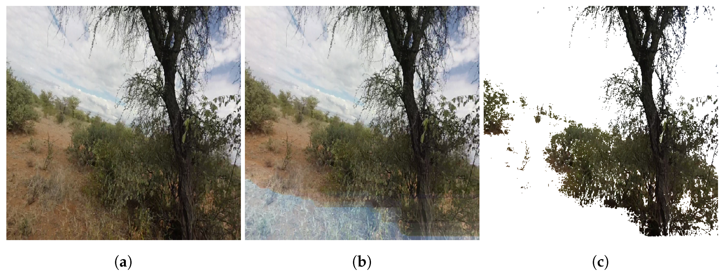Figure 5a shows a noisy image in which the contrast was non-ideal. In Figure 5b, the removal of undesired contrast regions is demonstrated, and finally, in Figure 5c, the color segmented result is displayed, where all grass, sand, and sky are removed.

From the filtered images, information now needed to be extracted, such that the RF could be trained to predict the labels of classes. It was found that the histogram feature extractor worked exceptionally well on the dataset. This step is indicated by “Extraction” in Figure 4. In computer vision, a histogram represents the pixel intensity distribution of an image. 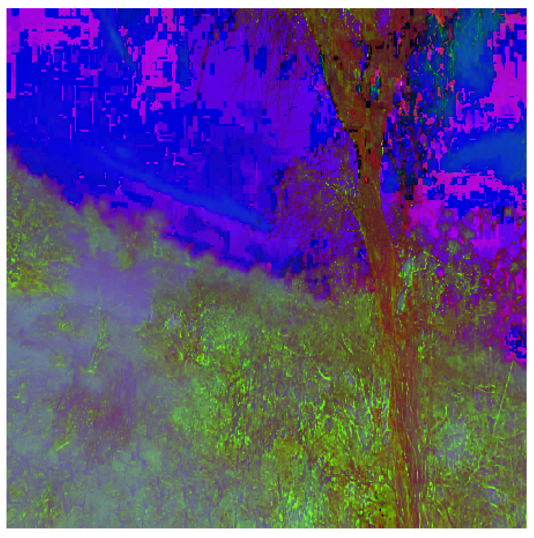If the histogram’s bins are chosen to collect every possible intensity occurrence, a histogram would range from 0–255 [28]. This information was used to gain knowledge about the contrast, intensity distribution (tonal range), and brightness. It was found that extraction from filtered HSV images worked well, as bushes were represented in bright green color and wood/trees in dark red. Such an unfiltered representation can be seen in Figure 6. Furthermore, histogram bin sizes of 3, 4, and 8 were shown to extract data suitable from which the RF could learn. In short, training was done by filtering the images twice, first to remove undesirable contrast areas and a second filter serving to remove sand, grass, and sky patches in the images. With a histogram feature extractor, a feature vector was gained, which could then be used to train an RF classifier.

Scaling and encoding showed that the extracted features were scaled between zero and one. Scaling was necessary, as the ML algorithm could optimally recognize patterns if the features were within a set range. The labels were encoded from alphabetical names to numerical values, such that they were usable by the ML algorithm. All these values were then stored during the Save Features operation under the .h5 format, suitable for large matrices. The operation RSCV means Randomized Search Cross-Validation, which was a hyperparameter-tuning method for the ML. Here, the hyperparameter space was randomly searched for the best cross-validation score. The hyperparameters tuned were “number of estimators”, “minimum samples to split”, “maximum forest depth”, a binary decision for “bootstrapping”, and a classification minimization “criterion”. The details of the hyperparameters were described by [23].

After tuning the ML hyperparameters, the plant identification operation started. Here, eighty new testing images were extracted from video streams and were used to test the classifier. The video camera was mounted to a car to prove the concept of the monitoring tool, and images were extracted from the video sequence at every 10^th frame. At a car speed of approximately 25 $\mathrm{k}$$\mathrm{m}$/$\mathrm{h}$ and a frame rate of 30 frames/s, each image covered $2.31$ $\mathrm{m}$. A filter was again applied to these images, which removed all the noise. During the search, a sliding window was applied to the image. The area in the window was converted to the HSV color space before the histogram feature extractor was applied. In summary, the search method consisted of first tuning the hyperparameters of the RF with the training data. The test images had to be filtered in a similar fashion as in the training section so that comparable results could be obtained. Searching then commenced after filtering using a sliding window technique on the filtered images, but in the HSV color space, as the taxonomies showed distinct features in this color space. Search results were stored and conditioned for the Output stage.

With this information, the RF could predict the class. RF was chosen as the ML algorithm, after testing a total of six algorithms. Testing was conducted on a small dataset comprised of unfiltered images with only the two tree classes. This was done to pre-select an ML-algorithm, which best performed on a similar dataset. The preconditioning and preprocessing of the entire dataset would then only focus on a single algorithm and not on an entire range, which saved time. Algorithm pre-selection was done according to a fivefold training set cross-validation score, conducted on 1000 images, 500 images per class. All classifiers tested during this stage and their cross-validation score are listed below, where the cross-validation score is indicated in brackets. As is evident from this list, RF was at this stage already the best performing algorithm, such that all other classifiers were rejected.

• Logistic regression (0.962).
• Gaussian naive Bayes (0.729).
• Linear discriminant analysis (0.968).
• K-Nearest neighbor (0.968).
• Support vector classifier (0.959).
• Random forest (0.970).

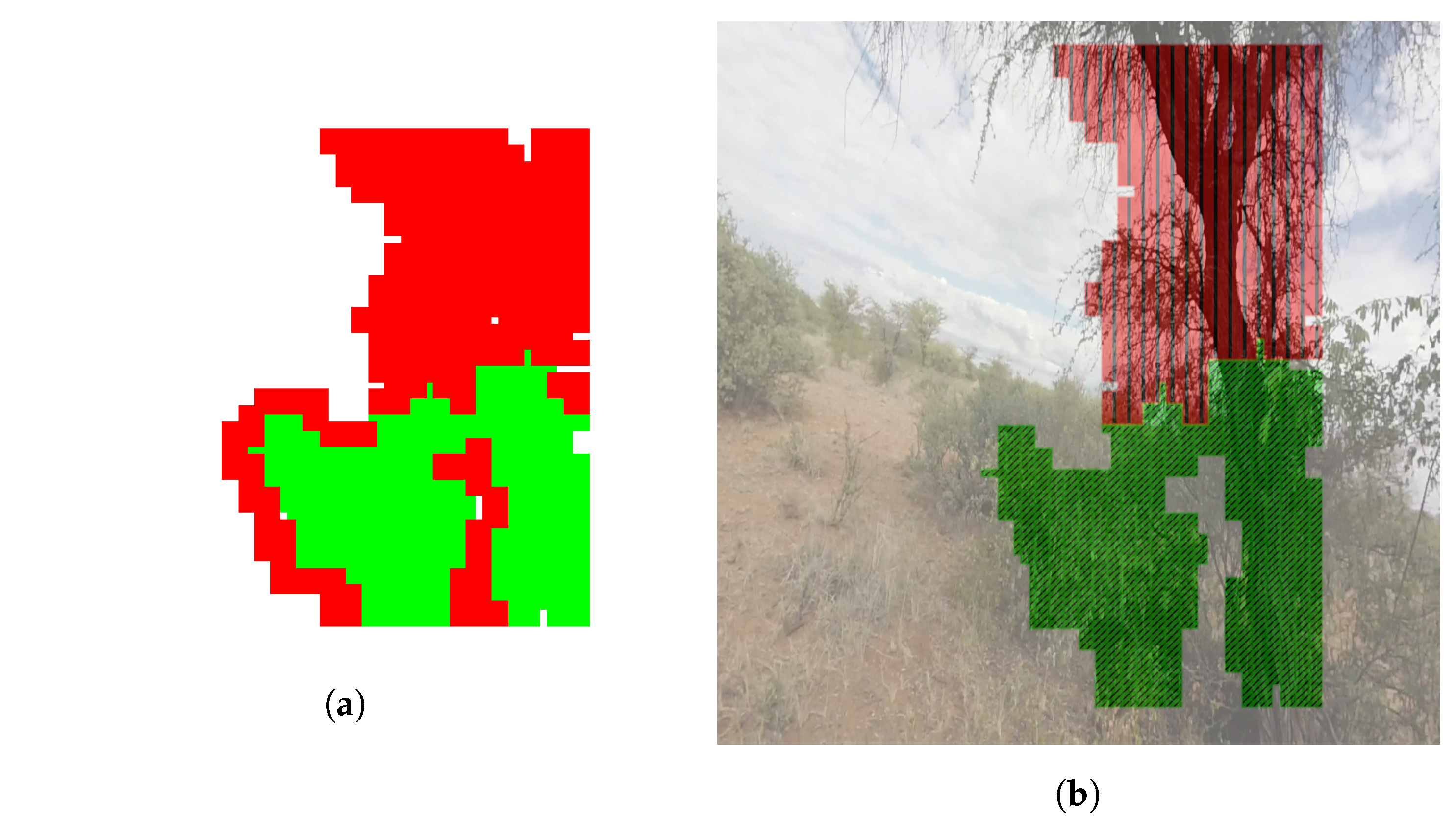
If one of the two classes was found, the coordinates and the width and length of the sliding window were saved during the Search Results operation as a .txt file. After all images were analyzed, the stored data from the .txt files were used to map out regions, where the instances found were mapped onto empty images. The output from this technique was a mixture of regions, where foliage and tree classes were identified. For example, if there was a tree in the center of an image, the program would identify the leaves as foliage and the branches and stems as wood. To obtain a uniform output, the Simple Linear Iterative Clustering (SLIC) [29] algorithm was used. SLIC is a method where similar pixels are clustered into superpixels so that image regions that contain similar information are grouped. This simplified the image representation and reduced the runtime during the identification procedures, as the image as effectively reduced from eight mega pixels to only a few superpixels. This resulted in a homogeneous region of interest, summarizing the most prevalent class. The final region of interest can be viewed in Figure 7, where red, vertically hatched areas indicate that the wood/tree class was found and green, diagonally hatched regions show that the foliage/bush classes were identified.

The output from this program was an area output. This was a bar chart that indicated on its ordinate the fraction of image area covered by each class. The abscissa showed the distance covered by the vehicle, calculated with the assumption that the car was traveling at 25 $\mathrm{k}$$\mathrm{m}$/$\mathrm{h}$. The bar chart output of a video-stream analysis can be viewed in Figure 8. This successfully indicated areas where a large quantity of foliage was present (green with diagonal hatching). This meant that these areas had a high biomass yield potential. Furthermore, the red carets show that there were images where wood was present, which indicated that there were trees in these images, and therefore, caution was advised when harvesting. This program sufficiently proved the concept that a monitoring tool could be created that could identify foliage and woody areas. Above the image, sample images from the sequence are shown, which corresponded to the abscissa indices, i.e., the first image was taken at 0 m distance covered, and the second image corresponded to 32 m covered. All codes were published and are publicly available under [30]. In conclusion, the Output stage finalized the label of the found regions of interest. For this, the SLIC algorithm was used as it pre-determined similar regions. Predominant regions were then colored with their corresponding labels, as determined by SLIC. The user then received an output chart, indicating biomass yield areas and areas with a high probability of protected species occurrence.

The developed program worked with sufficient accuracy within its environment. For the performance measure, the program decision boundaries were compared to ground truth boundaries. For this, ground truth boundaries were manually drawn on the test sequence, and the number of correlating program decision boundaries’ pixels was recorded in confusion matrices for each image. Correlating pixels were found using the accuracy score as displayed in Equations (1) and (2) [31,32]:

$$\mathrm{accuracy}=\frac{\mathrm{number}\mathrm{of}\mathrm{correct}\mathrm{predictions}}{\mathrm{number}\mathrm{of}\mathrm{predictions}},\mathrm{or}$$

(1)

$$\mathrm{accuracy}=\frac{\mathrm{TP}+\mathrm{TN}}{\mathrm{TP}+\mathrm{TN}+\mathrm{FP}+\mathrm{FN}}$$

(2)

In the above equation, TP, TN, FP, and FN are True Positive, True Negative, False Positive, and False Negative, respectively. The computation of this metric was simple and fast and allowed for a rapid evaluation of the model’s accuracy. A final confusion matrix was computed by taking the sum of all individual matrices. Each image contained $1\times {10}^6$ pixels, so that the entire validation sequence of 40 images contained $40\times {10}^6$ pixels. In these images, a total of $13.3\times {10}^6$ pixels represented the class, where $6.18\times {10}^6$ pixels represented the foliage class and $7.14\times {10}^6$ pixels represented the wood class. All remaining pixels formed areas where noise existed. Taking the total of all class-representing pixels as the basis of a confusion matrix, the following fractions could be determined:

• correct classification: the ground truth correlated with the prediction.
• incorrect classification: the ground truth differed from the prediction.

3. Results and Discussion

The confusion matrix is displayed in

Table 1. Confusion matrix evaluating the classification program.

		Ground Truth
		Foliage	Wood	Total
Predicted	Foliage	4,333,009	1,320,033	5,653,042
	Wood	1,845,435	5,819,893	7,665,328
	Total	6,178,444	7,139,926	13.3 × 106

, below. The values within the matrix display the actual number of pixels for correct classification, indicated in blue, and misclassification, indicated in black.

When computing the sum of all blue entries and dividing this result by the total number of pixels, the probability of the program classifying correctly could be determined. This probability was found to be 76%. Similarly, the probability of misclassification was determined to be 24%. The user’s accuracy for the foliage class was determined to be 77%, and for the wood class, this accuracy value was 76%. Furthermore, the producer’s accuracy for the foliage and wood class was 70% and 82%, respectively. Comparing these results with the results obtained by [6] for the classification, where the entire plant was used, the developed tool worked well. The accuracy reached in their study was 60%. This evaluation indicated that the concept was proven, such that the Namibian encroacher bush could be monitored using established computer vision technologies.

Misclassification occurred due to the chosen feature extraction technique. Tree canopies were classified as foliage because they appeared in green color tones as opposed to the red stems. If a canopy was large, then the superpixel algorithm clustered the entire canopy as a bush. Other reasons could include that there were still not enough data available in the dataset. These problems could possibly be overcome with the use of a neural network. Here, the algorithm automatically identified features within the images so that there was no error made by changing the color spaces and retrieving information by a histogram.

This method was limited to its dataset. The set was taken during the winter period, where the background was relatively homogeneous, as compared to the summer months. During summer, flowers would appear in the images, which would add to the background noise. Furthermore, all images were taken on days where there were cloudy skies present. The algorithm would probably not work as good on images with clear skies. These problems would be overcome by extending the dataset with images taken throughout the year.

The fact proven by this project, that computer vision could be used in bush and tree identification, implied that this concept could also be used in autonomous harvesting. Here, a robot would be used to harvest the encroacher bush, instead of a human. This could improve the process efficiency and reduce harvesting costs. Future improvements of the method would incorporate the use of image pyramids. This would improve classification accuracy and eliminate the current aspect problem, i.e., the actual size of the plant and the distance of the camera from the plant [33].

Bush encroachment in Namibia has lead to severe economic and biodiversity loss, as well as land degradation. It was shown that through harvesting this biomass, within the legislative framework of the Namibian government, sustainable products were created; either electricity or charcoal. However, the current harvesting methods were not selective enough to comply with the government recommendation. Computer vision could bridge the gap between economic and sustainable harvesting, as it could be used to distinguish taxonomies so that no protected species are harvested. The concept of the monitoring tool was successfully proven, which indicated that with simple computer vision libraries, a correct classification accuracy of 76% could be achieved. Software was developed that could comply with the regulations. The developed concept proved that the Namibian encroacher bush could be monitored with established technologies, to both benefit the economy and the environment.