A Hybrid Predictive Approach for Chromium Layer Thickness in the Hard Chromium Plating Process Based on the Differential Evolution/Gradient Boosted Regression Tree Methodology

Abstract

The purpose of the industrial process of chromium plating is the creation of a hard and wear-resistant layer of chromium over a metallic surface. One of the main properties of chromium plating is its resistance to both wear and corrosion. This research presents an innovative nonparametric machine learning approach that makes use of a hybrid gradient boosted regression tree (GBRT) methodology for hard chromium layer thickness prediction. GBRT is a non-parametric statistical learning technique that produces a prediction model in the form of an ensemble of weak prediction models. The motivation for boosting is a procedure that combines the output of many weak classifiers to produce a powerful committee. In this study, the GBRT hyperparameters were optimized with the help of differential evolution (DE). DE is an optimization technique within evolutionary computing. The results found that this model was able to predict the thickness of the chromium layer formed in this industrial process with a determination coefficient equal to 0.9842 and a root-mean-square error value of 0.01590. The two most important variables of the model were the time of the hard-chromium process and the thickness of the layer removed by electropolishing. Thus, these results provide a foundation for an accurate predictive model of hard chromium layer thickness. The derived model also allowed the ranking of the importance of the independent input variables that were examined. Finally, the high performance and simplicity of the model make the DE/GBRT method attractive compared to conventional forecasting techniques.

1. Introduction

Hard chromium plating consists of the electroplating of existing chromium into a solution containing chromic acid and a catalytic anion in the appropriate proportion. The deposited metal forms a layer of extreme hardness and corrosion resistance. Commercial hard chromium plating originated in patent 1,581,188 of the United States Patent Office, registered by Colin Fink on April 20, 1926 [1]. The main differences of hard chromium plating and decorative chromium plating are as follows [2]:

• Hard chrome deposits are mainly used to increase the service life of functional parts, as they increase resistance to wear as well as abrasion, heat and corrosion. These deposits are also applied to the parts to recover their dimensions when they are under nominal measurement.
• Hard chromium is deposited in thicknesses ranging from 2.5 to 500 μm and, in certain cases, with greater thicknesses, while decorative chromium plating seldom exceeds 1.5 μm.
• Hard chromium plating is normally applied directly to the base metal while decorative chromium plating is deposited over precoatings of nickel or copper-nickel alloys.

The conventional chrome plating bath contains chromic acid and sulphuric acid in a proportion of 100 to 1, respectively. The chromic acid is broken down electrolytically to form a chromium film on the part to be treated. Approximately 20% of the current passing through the bath is used to produce chromium. The remainder is used in the deionization of the water. The chromic acid found in the bath is formed from chromium trioxide and water by the reaction [3]:

CrO₃+H₂ O ⇔H₂ CrO₄.

The role of the two acids inside the bath can be represented by the following balance:

100 H₂ CrO₄ + H₂ SO₄ ⇔ 100 Cr + 100 H₂O + 150 O₂ + H₂SO₄.

These elementary reactions take place in both senses. It should be noted that the hard chrome plating bath is operated with an anode which is insoluble and therefore does not need to be replaced.

The sulphuric acid remaining in the bath is the catalyst and is essential for the coating to take place [3]. It must be present within very specific limits to control the characteristics of the electroplating. In all chrome plating baths the metal comes from chromic acid, but the chromic acid solution does not deposit chromium unless there is a certain amount of catalyst [4]. If the catalyst concentration is too high or too low the chromium will not deposit. Acid anions have been shown to serve as catalysts [4]. Sulphate was the first to be used. The replacement of part of the sulphate with fluoride ions, present in the complex acid radicals, improves the chromium plating operations [5]. Taking into account these two types of catalysts [6], chromium plating baths can be classified into conventional (sulphate) and catalyst (fluoride).

The composition of conventional sulphate baths may vary considerably, but the weight ratio of chromic acid to sulphate radical must be between 75 to 1 and 120 to 1 [7]. The deposition power or the current distribution of the deposit is optimal for ratios between 75 to 1 and 110 to 1. However, in the area between 75 to 1 and 90 to 1, brighter deposits are obtained and higher current densities may be used without the risk that an excess current applied may result in point burning on the surface of the part.

Although solutions with very low concentrations of chromic acid (50 g/L) have been used, these are impractical as they have several disadvantages [2]:

• The thicknesses obtained are very limited.
• These solutions are very sensitive to contamination.
• Higher voltages are needed.

The low concentration bath is widely used because it is not only able to chrome faster than high-concentration baths but also reduces drag-out losses [2]. These are called losses due to the amount of fluid that comes out of the bath adhered either to the processed parts or to the frame. This amount of fluid is directly proportional to the surface tension of the solution.

The high-concentration bath has the advantage of being less sensitive to the contamination inherent to use in an industrial installation [8], is easier to control and has greater deposition power. Furthermore, having higher concentration is more conductive, so it can work at lower voltages and is heated less during operation.

If the available rectifier does not exceed 6 V, it may be preferable to work at higher concentrations of chromic acid (300 to 400 g/L), although the efficiency will be lower than with less concentrated solutions [2]. Lower efficiency is compensated by increased current density as a result of better conductivity. Normally, the best values to operate are between 200 and 300 g/L of chromic acid [2], bearing in mind that, within this range, solutions with 200 g/L have a higher (current) efficiency, while solutions with 300 g/L have better conductivity.

The conductivity of catalyst solutions is similar to that of conventional sulphate baths, but they produce harder deposits and have better efficiency [9] for identical working conditions (it also has better efficiency for higher concentrations). This type of bath can increase the production between 40 and 60% with respect to conventional baths, as they have greater efficiency and can operate at higher current densities without danger to the tank [9]. In addition, coarse deposits can be obtained without the formation of areas where the chromium plating thickness reaches values that lead to the appearance of spheroidal chromium grains on the surface of the part [2]. A limitation of baths of this type is that they can attack non-chrome surfaces in areas with low current density. This attack can be avoided by masking the areas that are not going to be chromium plated.

The main applications of hard chromium plating are related to those situations in which a high resistance to wear is required or in the cases in which the recovery is sought of parts that, due to wear and tear, have remained low in size [10].

There are numerous data [5,10] on the effectiveness of chromium plating in reducing segment wear (automotive) by combating friction wear, lack of lubricant and abrasion. The average life of a chromium-plated segment is about five times longer than that of a non-chromium-plated segment made of the same base metal [10]. The segments of most engines are chrome-plated with a thickness of 100 to 175 μm on the wear face, although it can reach 250 μm for some large engines.

In the automotive industry, hard chromium plating is also used for shock absorbers and suspension components, increasing their resistance to wear and corrosion. In the case of Western countries, despite the financial crisis suffered during the past decade, the automotive industry continues to have an important influence on wider industrial practices [11]. Valve rods are treated with a chromium layer of 0.25 μm to reduce wear and tear.

There are different reasons for recommending the chrome plating of tools [12]:

• Reduce wear and tear.
• Avoid seizures.
• Reduce friction.
• Prevent or reduce corrosion.

In the case of cutting tools, their life can be increased by hard chromium plating, with thicknesses ranging from 2.5 to 13 μm [12]. Hard chromium plating is sometimes used for the recovery of poorly machined parts or for parts subject to wear, such as the worn surfaces of large diesel engine shafts and compressors, due to its excellent wear-resistance properties and low coefficient of friction. In these cases, the thickness of the tank varies from about 125 to 1250 μm. Chromium deposition is usually avoided in threaded areas and in agreed radii to prevent fatigue breakage.

The decision to use hard chromium on a part must be based on the following considerations [5]:

• The hardness and wear resistance of hard chromium plating.
• The necessary chromium thickness.
• The shape, size and construction of the part to be chromed, as well as the kind of material from which it is constructed.
• The masking requirements for parts that are not fully chrome plated.
• Dimensional requirements (if further machining is required and if it can be carried out according to the indicated tolerances).

The hardness of chromium electrodeposits depends on the conditions under which the chromium plating is carried out. In general, chromium plating in the bright range is harder [8]. Bright chrome deposits obtained in conventional baths have Vickers hardness from 900 to 1000, while those obtained in catalyzed baths have hardness from 1000 to 1100 or even higher [12].

It is common for large pieces to be covered by parts, or by rotating them in such a way that at a given moment only a part of the piece remains submerged. This has been used for shafts up to 4 m in diameter and 18 m in length [5]. When this technique is used, the whole area of the part that is to be chromed and remains exposed to the atmosphere must be wet with the chroming solution.

Today, there is significant industry experience in the use of hard chromium plating as a roller coating in rolling mills. This experience shows that the average life of the rollers coated in this way is higher than that of those without the treatment [3]. From a mechanical point of view, the properties of electrodeposited chromium are similar to those of metal chromium [5]. The most important of these are its great hardness, low coefficient of friction, good corrosion resistance, low coefficient of thermal expansion and high conductivity.

There are a number of basic requirements that must be met in order for hard chrome plating to achieve its maximum effectiveness [5]:

• The base material on which the coating is applied must be such that it can withstand the external forces applied with minimal deformation. That is, the properties of the base material must be similar to those of the applied chromium layer.
• The thickness of the chromium layer should be reduced to a minimum in those areas of the part that are expected to have a high deformation. If this is not done, the chromium layer should be reduced to a minimum in those areas of the part that are expected to have a high deformation. If this is not done, this will favor the chromium layer to be chromium.

Finally, it is also necessary before choosing hard chrome plating as a coating method for a part to consider whether there is another industrial process that provides the same result in a less polluting way. For example, the hard chromium plating traditionally used to restore the shafts of aeronautical turbines to their original diameter is beginning to be replaced by other processes, such as so-called HVOF (high-velocity oxy-fuel), which is less harmful to the environment [13].

The aim pursued in this research is to assess the suitability of the gradient boosted regression tree (GBRT) model [14,15,16,17,18,19] to predict chromium layer thickness considering several variables from the industrial process. The goals of the model developed in this research are to overcome several problems currently found in industry and to enhance the in-depth knowledge of the industrial process as a whole.

GBRT models are a kind of machine learning model that has demonstrated effective performance for both regression and classification [15,16,17,18,19]. The GBRT models of the present research were trained to estimate the thickness of the chromium plating layer. GBRT models have proved to be successful in other disciplines, such as the prediction of biological parameters in environmental problems, solar power generation prediction [20] and waste estimation in the short-term [21].

Differential evolution (DE) is a metaheuristic evolutionary global method able to solve multidimensional optimization problems that makes use of continuous variables. It is a bio-inspired algorithm that makes use of operations such as mutation, recombination and selection [22,23,24,25].

So-called hard chromium plating consists of electrolytic deposits of relatively large thicknesses (0.1 mm) that are deposited on parts that must withstand great stresses of wear. This type of deposit is used particularly in valve seats, bearings, crankshafts, shafts of hydraulic pistons and, in general, in pieces where a high level of precision is required. Hard chrome plating is especially used in the grinding of internal combustion engines. Crankshafts and other fundamental parts of internal combustion engines suffer wear, causing looseness in their bearings which can compromise their operation. In order to avoid a serious break, lost metal parts are replaced by electrolytic chromium.

The set-up of any industrial process is mainly driven by the experience of the manufacturer. This is also the case of hard chromium plating. One of the most challenging tasks is the attainment of a chromium layer with the required thickness inside tolerance. There are three main methodologies to measure the thickness of the hard chromium layer. One consists of measuring the part before and after the plating; a second method is a destructive test, which requires cutting some pieces and measuring the thickness of the chromium layer with the help of an electronic microscope; and the third is the measurement of the thickness with the help of a device based on eddy currents [26,27] or in any ultrasonic non-destructive test [28]. Usually, during the process set-up, variables like current, voltage and process time are fixed according to piece geometry and the thickness of the layer required. During the process operation, those parameters, together with others [29] such as bath temperature, bath volume, and solution density, are controlled. The purpose of the use of a machine learning-based methodology in order to predict chromium layer thickness in the hard chromium plating process is two-fold: such an approach makes it easier, first, to set up a new industrial process and, second, to control how the thickness of the chromium layer changes according to the variations in the operation variables that are monitored. In other words, the aim of the proposed method is not to completely replace the measurement of the hard chrome layer by classical methods, but to also speed up the set-up process and reduce the required inspection frequency.

Although previous studies have dealt with the hard-chromium process from different points of view [7,12,13], with some even taking into account monitoring of real-time variables [29], as far as is known by the authors, few studies have made use of machine learning methodologies in this field [30,31] and none have employed the new DE/GBRT methodology.

In summary, the main objective of the present study was to develop a hybrid algorithm with DE optimization of GBRT parameters (DE/GBRT-based model) to predict the thickness of the hard chromium layer from the seven physical-chemical input parameters of the hard chromium plating process. The results obtained showed that the GBRT technique in combination with DE optimization can be used to build models with high performance for the estimation of the thickness of the hard chromium layer. Therefore, this methodology has demonstrated its usefulness for both the set-up and control of production lines.

2. Materials and Methods

2.1. Equipment and Experimental Dataset

There are some differences between chromium plating and other electroplating processes. In the case of chromium plating, the chromium deposition is achieved in different stages that consist mainly of the reduction of hexavalent chromic acid. The hard chromium plating process relies on four main stages: vapor degreasing, manual cleaning, electropolishing and the hard chrome process. Figure 1 shows a flowchart with the main stages of the industrial hard chromium plating process. These stages can be described as follows:

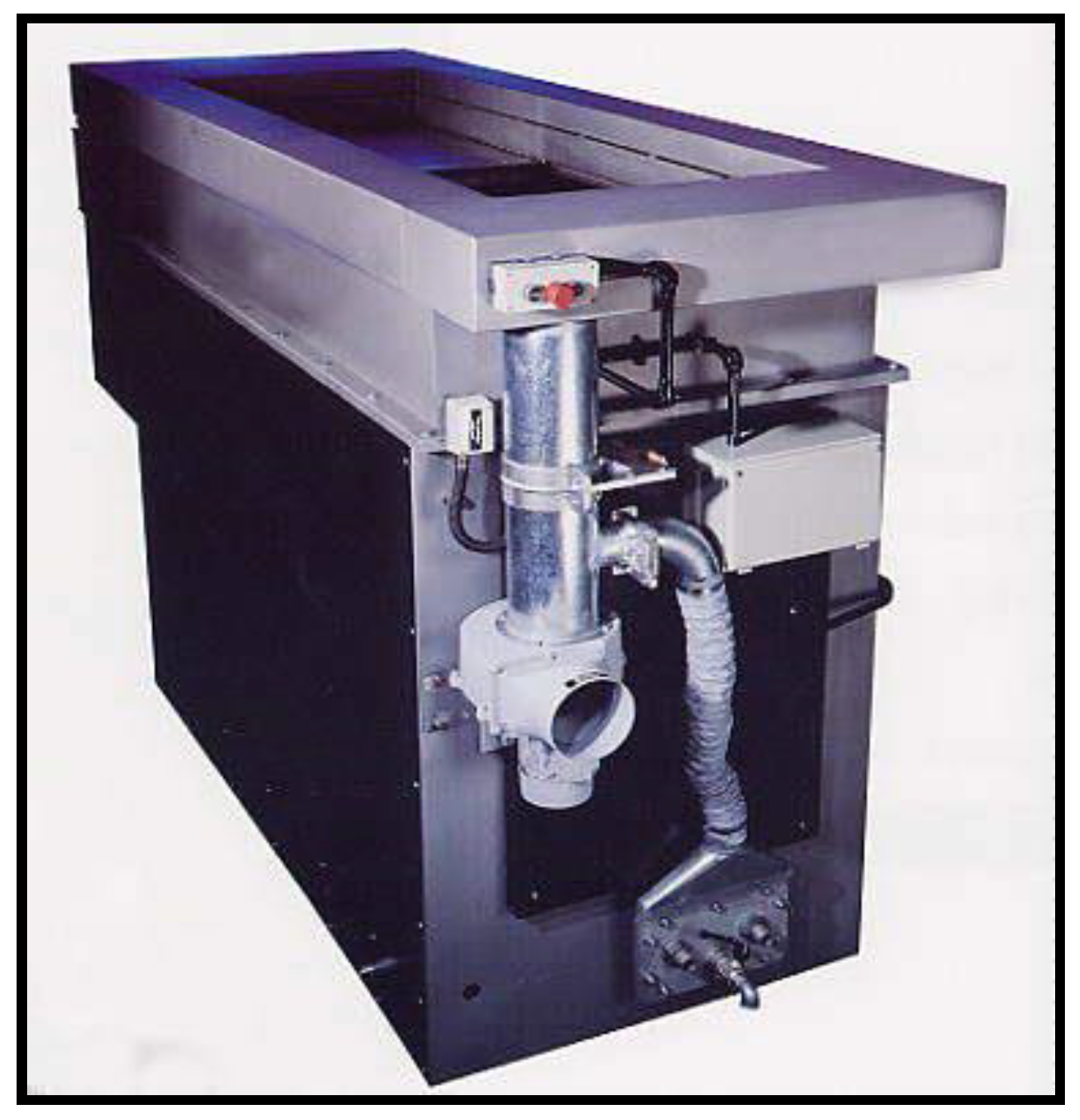
• Degreasing in the vapor phase: Degreasing in the vapor phase is carried out in a tank built of stainless steel (see Figure 2). The pipes to be degreased are fastened in special frames made of corrosion resistant materials and are slowly introduced into the interior of the tank. These pieces must be free of water and moisture prior to degreasing. The immersion time is 10 min, which is sufficient time for the pieces to reach the temperature of the steam. It can be verified that this temperature has been reached because the steam does not condense on the lower surfaces of the pieces.
• Manual cleaning: During this stage, all residual traces of dirt and surface impurities are cleaned by hand.
• Electropolishing: The electropolishing operation consists of the following phases: Cleaning with acetone and dry wick (phase 1): cleaning with acetone consists of the introduction inside the piece of a wet wick soaked with acetone twice. To complete the cleaning, a dry wick is subsequently also inserted twice. Load (phase 2): the pieces are placed in the frames provided with a feeder and the anodic rod that passes through it. Then, the connector tool is placed on the piece while the anodic rod is fixed with a screw and tensioned by operating the upper cam. Finally, the tool is electrically connected by means of a cable. Electropolishing (phase 3): for each electropolished load, the system records the minimum, maximum and average temperature values. Normally, the electropolishing time varies depending on the material to be removed. Recycled wash (phase 4): recycled washing means washing with watertight water. This water is changed once every 6 months. The pieces are washed during an immersion time between 0.5 and 2 min. Washing with recirculation (phase 5): in order to achieve complete degreasing, the washed pieces are now washed in a bath of demineralized water at room temperature for a time between 1 and 3 min. Removal of the support (phase 6): after washing in demineralized water, the pieces of the frame are disassembled. To do this, an operator removes them one by one, proceeding subsequently to clean them. Visual inspection (phase 7): the electropolished pieces are inspected visually, verifying the absence of dirt and pollution for all of them.
• Hard chromium process: the hard chrome operation consists of the following phases: Cleaning the chromed pieces (phase 1): Immediately before the chrome operation, the pieces are cleaned with a pressurized water gun. Next, each piece is blown with pressurized air to remove the remains of water. Load (phase 2): The pieces to be chromed are placed in the corresponding frame provided with the feeder. Hard chrome process (phase 3): The chroming of the pieces is carried out by immersion in a bath operating under the following conditions: (a) working temperature between 53 and 56 °C; (b) concentration between 238 and 278 g/L; and (c) agitation of the bath by means of air through a coil. Recycled washing (phase 4): this phase involves washing with watertight water at room temperature for a time between 1 and 3 min. Washing in demineralized water (phase 5): the pieces are washed by immersion in a bath of demineralized water at room temperature for a time between 1 and 3 min. Immersion in tank with sodium hydroxide (phase 6): Once the pieces are removed from the frame, they are washed with water and introduced into an alkaline bath. The minimum time in this bath is three minutes. After this time, they are extracted from the bath and washed by hand with water.

In this study, eight process variables were collected from the hard chrome plating process, including the dependent variable (thickness of the hard chrome layer). The seven input variables are briefly described in

Table 1. Set of operation physical input variables used in this study and their names, with their mean and standard deviation.

Input Variables	Name of the Variable	Mean	Standard Deviation
Iron content of the electropolishing bath (mg/L)	iron_ep	0.1218	0.0942
Electropolishing time (minutes)	ep_time	4.5064	0.9066
Electropolishing bath temperature (°C)	ep_temp	53.595	4.6207
Layer thickness removed by electropolishing (μm)	thick_electropol	305.95	34.464
Chromic acid content (g/L)	chrom_acid	240.68	8.7120
Hard chromium process time (minutes)	hard_chrom_time	30.761	3.3272
Hard chrome bath temperature (°C)	hard_chrom_temp	53.962	0.4696
Chrome thickness (mm)	Thickness_chrom	6.5920	0.2069

. The total number of datapoints used in this study was 37,360. The output variable (or dependent variable) considered in this study was the hard chromium plating thickness (in microns).

The aim of this study was to determine the relationship between the thickness of the hard chromium layer (dependent variable) in microns and the operation physical-chemical input variables (independent variables); these operation input variables are described below:

• Iron content of the electropolishing bath (mg/L): iron content in the electropolishing bath expressed in mg/L.
• Electropolishing time (minutes): this variable represents the amount of time, expressed in minutes, that the part is submerged in the electropolishing bath.
• Electropolishing bath temperature (°C): this variable expresses the electropolishing bath temperature in degrees Celsius. Due to the electropolishing process, the bath temperature increases. A high bath temperature reduces the performance of the electropolishing process.
• Layer thickness removed by electropolishing (μm): the electropolishing process causes the removal of a certain amount of material. This variable measures the amount of material removed.
• Chromic acid content (g/L): chromic acid content in the hard chromium bath expressed in g/L.
• Hard chrome plating time (minutes): after the electropolishing operation, the part is submerged in the hard chromium plating bath. This variable measures the time of immersion.
• Hard chrome plating temperature (°C): this variable expresses the chrome plating bath temperature in degrees Celsius. As for electropolishing, in this case due to the electrolytical process, the bath temperature increases. The bath temperature influences the operation performance.

Figure 3 shows an overview of the eight sample variables over time.

2.2. Computational Procedure

The first stage of the analysis consists of a correlation matrix of all the variables. The graphical results are presented in Figure 4. The correlation matrix shows almost no correlation between independent variables, and some correlation of the dependent variable thickness of the hard chrome layer (thickness_chrom) with input variables layer thickness removed by electropolishing (thick_electropol) and hard chromium process time (hard_chrom_time). This result highlights the difficulty with obtaining predictive models using linear regression methods. Therefore, it is necessary to tackle this complex problem with more advanced nonlinear techniques relying on statistical machine learning, such as the evolutionary gradient boosted regression tree (DE/GBRT-based model) method used in this study.

2.2.1. Gradient Boosted Regression Tree (GBRT)

Gradient boosting (GB) is a statistical machine learning method originally designed for classification problems and later effectively extended to regression problems. The main motivation behind this technique is the possibility of combining many weak models (or learners) to derive a powerful ensemble (or committee). This technique constructs the model in stages, characteristic of the boosting methods, so that a unique and powerful ensemble model is obtained by optimizing a suitable differentiable loss function [14,15,16,17,18,19,32,33].

For example, we can consider the least-squares error as a loss function, for which the purpose is to educate an F model to estimate the true values y from the training subset as the foretold values $\widehat{y}=F\left(x\right)$, in such a way as to minimize the error ${\left(\widehat{y}-y\right)}^2$.

The key idea is as follows: Assume that we have a weak model $F_m$ to forecast the mean y of the training subset in each stage m of gradient boosting (with m ranging from 1 to M). Next, the GB algorithm ameliorates $F_m$ by creating a novel model $F_{m+1}$, adding an estimator to ameliorate the earlier model $F_{m+1}\left(x\right)=F_m\left(x\right)+h\left(x\right)$. In this way, to derive a perfect h, the gradient boosting algorithm is subject to [17,18,19,34]:

$$F_{m+1}\left(x\right)=F_m\left(x\right)+h\left(x\right)=y$$

(1)

or, equivalently:

$$h\left(x\right)=y-F_m\left(x\right).$$

(2)

Then, the GB method carries out the fitting of h to the residual $y-F_m\left(x\right)$. Therefore, the model $F_{m+1}$ corresponding to the following stage, is obtained by improving its predecessor $F_m$. It is possible to generalize this technique to other loss functions other than the least-squares error $\frac{1}{2}{\left(y-F\left(x\right)\right)}^2$, keeping in mind that residuals $y-F\left(x\right)$ are the negative gradients of this previous loss function.

With this background, the pseudocode of the gradient boosting algorithm is given as follows [19,32,33,34]:

➢

Input requirements: the training set ${\left\{\left(x_i,y_i\right)\right\}}_{i=1}^n$, maximum iteration number M (as the algorithm stopping criterion) and a differentiable loss function $L\left(y,F\left(x\right)\right)$.

➢

Steps of GB algorithm:

• Begin the model with a constant value:

  $$F_0\left(x\right)=\underset{\gamma }{\arg \min }{\displaystyle \sum _{i=1}^{n}L\left(y_i,\gamma \right)}$$
• A loop from $m=1\mathrm{to}M$:
  • Calculate the pseudo-residuals with the negative gradient:

    $$r_{im}=-{\left[\frac{\partial L\left(y_i,F\left(x_i\right)\right)}{\partial F\left(x_i\right)}\right]}_{F\left(x\right)=F_{m-1}\left(x\right)}\mathrm{for}i=1,\dots ,n$$
  • Fitting phase: a weak learner $h_m\left(x\right)$ is fitting to the pseudo-residuals using the training set ${\left\{\left(x_i,r_{im}\right)\right\}}_{i=1}^n$.
  • Computation of the multiplier ${\gamma }_m$ by solving the following one-dimensional optimization problem:

    $${\gamma }_m=\underset{\gamma }{\arg \min }{\displaystyle \sum _{i=1}^{n}L\left(y_i,F_{m-1}\left(x_i\right)+\gamma h_m\left(x_i\right)\right)}$$
  • Upgrade the model:

    $$F_m\left(x\right)=F_{m-1}\left(x\right)+{\gamma }_m{h}_m\left(x\right)$$

    (3)
• End: obtain $F_M\left(x\right)$.

Most commonly, the gradient boosting technique uses regression trees (RTs) with a given size as weak learners [19,34,35,36]. Indeed, in each GB algorithm iteration, a RT is fitted to the present residuals. If a sufficient number of regression trees is taken into account in the final model, then an arbitrarily small training error results; that is, the overfitting of the training set can cause a bad prediction ability of the model. To avoid overfitting, it is appropriate to apply a simple regularization strategy resizing the weight of each RT by a quantity $\eta$:

$$F_m\left(x\right)=F_{m-1}\left(x\right)+\eta \cdot h_m\left(x\right)\hspace{1em}\mathrm{with}\hspace{1em}\eta \in \left[0,1\right].$$

(4)

The parameter $\eta$ in Equations (3) is also termed the learning rate because it shrinks the contribution of each new weak learner (or base model) that is added in the series. Therefore, $\eta$ is greatly related to the maximum number of boosting iterations M. Empirical evidence implies that better testing errors are obtained from low M values. Hastie et al. 2009 [19] advises fixing the learning rate at a small constant and choosing M to stop before this value.

Furthermore, typical hyperparameters of the GBRT technique can be outlined as [37,38]:

• Nrounds (M): Maximum number of iterations of the GB algorithm.
• Learning rate $\eta$: This algorithm resizes the weight of each RT by a factor $\eta$ when it is added to the present approximation. This factor avoids overfitting since the GB algorithm becomes more resistant to change. It is well known that a smaller value of $\eta$ requires a greater Nrounds value.
• $\gamma$: Minimum loss drop necessary to carry out another partition on a RT leaf node. Note that if this parameter grows, the algorithm is more resistant to change.
• Minimum child weight: Minimum sum of weight (Hessian) necessary for a child.
• Maximum $\Delta$ step: Limit value in the contribution of each tree.
• Subsample ratio: The relative proportion between the training and testing samples.

Hence, it is suitable to employ mathematical methods that determine these hyperparameters accurately. In this study, the differential evolution (DE) optimization approach explained below was utilized [22,25] with a satisfactory outcome.

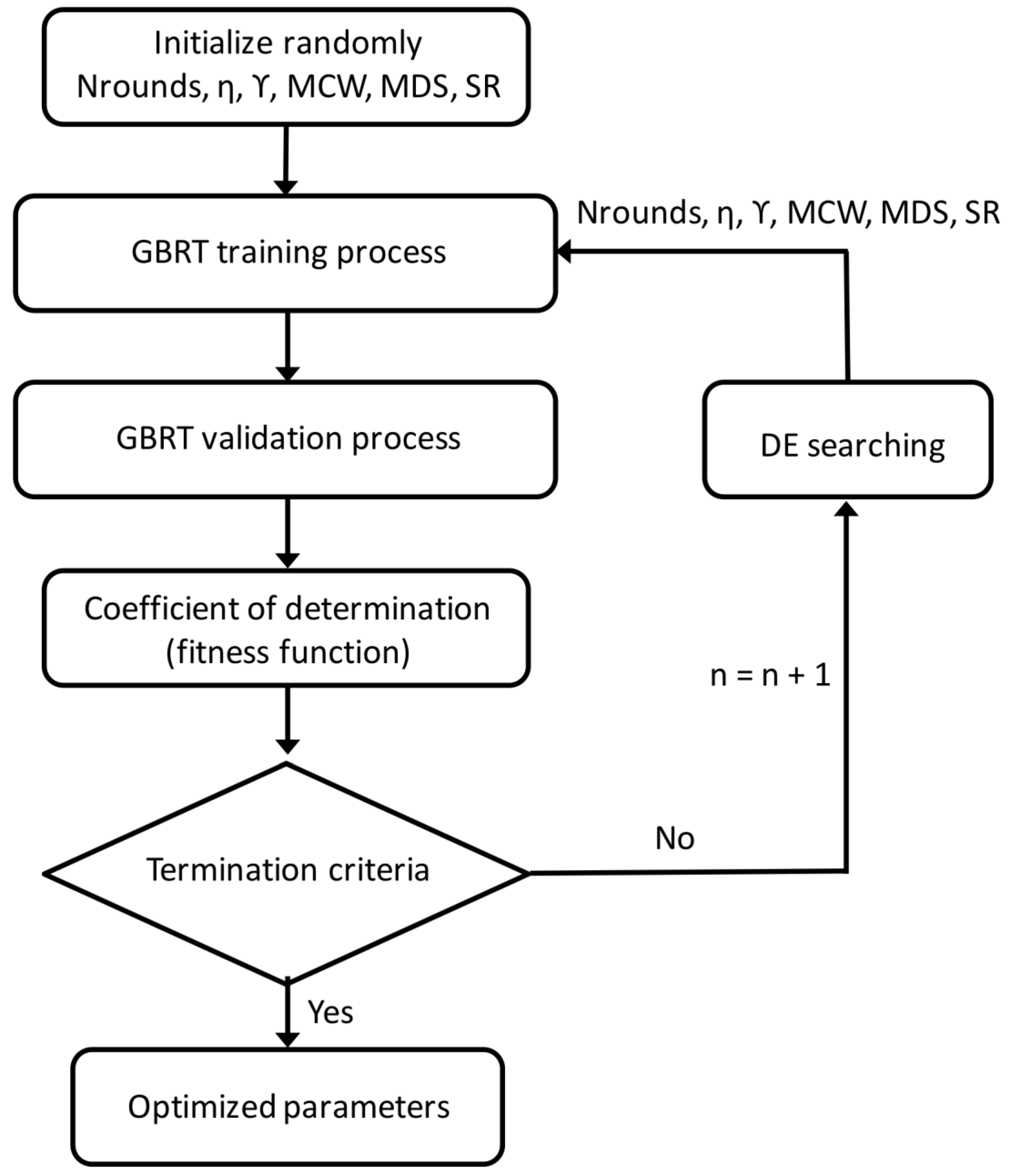
2.2.2. Differential Evolution (DE) Algorithm

Differential evolution (DE) is an optimization method within evolutionary computing, applied in solving complex problems. Like other algorithms in this category, DE maintains a population of candidate solutions, which are recombined and mutated to produce new individuals that will be chosen according to the value of their performance function [22]. DE is characterized by the use of test vectors, which compete with individuals in the current population in order to survive. The first research work on the DE technique was developed by Storn and Price [22,23]. Originally, the method was focused on solving Chebyshev’s polynomial fitness problem using a variant of the method called Genetic Annealing (GA), which had been developed by Price the previous year [22,23,24,25].

The DE algorithm assumes that the variables of the problem to be optimized are encoded as a vector of real numbers. The length n of these vectors is equal to the number of problem variables and the population is composed of NP (number of parents) vectors. A vector $x_p^g$ is defined, where p is the index of the individual in the population $\left(p=1,\dots ,NP\right)$ and g is the corresponding generation. In turn, each vector is composed of the variables of the problem $x_{p,m}^g$, where m is the index of the variable in the individual $\left(m=1,\dots ,n\right)$. It is assumed that the domain of the problem variables is restricted between minimum and maximum values $x_m^{\min }$ and $x_m^{\max }$, respectively.

The DE algorithm is basically composed of 4 steps [22,23,24,25,39,40]:

• Initialization: this stage is performed at the beginning of the search run. Indeed, the population is initialized (first generation) randomly, considering the minimum and maximum values of each variable:

  $$x_{p,m}^1=x_m^{\min }+\mathrm{rand}\left(0,1\right)\cdot \left(x_m^{\max }-x_m^{\min }\right)\mathrm{for}p=1,\dots ,NP\mathrm{and}m=1,\dots ,n$$

  (5)

  where $\mathrm{rand}\left(0,1\right)$ is a random number in the range [0, 1].

Next, the mutation–recombination–selection steps are repeated, until a term condition is satisfied (number of generations, elapsed time, or quality of solution reached, among others).

• Mutation: this stage consists of the construction of NP noisy random vectors, which are created from three randomly chosen individuals $x_a$, $x_b$ and $x_c$, termed target vectors. Noisy random vectors $n_p^t$ are obtained as follows:

  $$n_p^g=x_c+F\cdot \left(x_a-x_b\right)\mathrm{for}p=1,\dots ,NP$$

  (6)

  in which p, a, b and c different from each other. Furthermore, F is a parameter that controls the mutation rate and is in the range [0, 2].
• Recombination: once the NP noisy random vectors are obtained, recombination is carried out randomly, by comparing them with the original vectors $x_{p,m}^g$, obtaining the trial vectors as follows:

  $$t_{p,m}^g=\left\{\begin{array}{ccc}{n}_{p,m}^g& \mathrm{if}& \mathrm{rand}\left(0,1\right)<GR\\ x_{p,m}^g& & \mathrm{otherwise}\end{array}\right\}\mathrm{for}p=1,\dots ,NP\mathrm{and}m=1,\dots ,n.$$

  (7)

  GR is a parameter that controls the recombination rate. Note that the comparison is made variable by variable, so that the trial vector will be a mixture of the noisy random vectors and original vector.
• Selection: Finally, the selection stage is carried out simply by comparing the trial vectors with the original vectors, so that the next generation vector will be that with the best performance fitness value fit:

  $$x_p^{g+1}=\left\{\begin{array}{ccc}{t}_p^g& \mathrm{if}& fit\left(t_p^g\right)>fit\left(x_p^g\right)\\ x_p^g& & \mathrm{otherwise}\end{array}\right\}\hspace{1em}.$$

  (8)

The Xgboots package of the statistical software R [37,38,41], in conjunction with the DE technique in the DEoptim package [25,40,42], were used to construct the final regression model. An iMac with a 3.2 GHz Intel Core i5 processor and 8 GB of RAM was used in the computations. Approximately 32 h were needed to complete the hyperparameter tuning selection using a population of 60 individuals with a stopping condition of 30 steps without improvement and a maximum number of 200 iterations. The solution was reached after 95 iterations.

2.3. The Goodness-of-Fit of This Approach

In the present research, a DE/GBRT-based model was used to estimate the thickness of the hard chrome layer applying a regularized method [17,18,19,34,35]. The goodness of fit of a regression model is a measure of the quality of the model that takes into account the discrepancies between the real and forecasted values. The main goodness-of-fit parameter used in this work was the coefficient of determination R² [19,43]. If the observed values are $t_i$, the corresponding modelled values are $y_i$ and $\overline{t}$ is the mean of the n observed samples:

$$\overline{t}=\frac{1}{n}{\displaystyle \sum _{i=1}^n{t}_i}.$$

(9)

The coefficient of determination is given by Equation (9):

$$R^2\equiv 1-\frac{{\displaystyle \sum _{i=1}^n{\left(t_i-y_i\right)}^2}}{{\displaystyle \sum _{i=1}^n{\left(t_i-\overline{t}\right)}^2}}.$$

(10)

If the coefficient of determination has a value of 1.0 it means that there is no difference between the predicted and observed data.

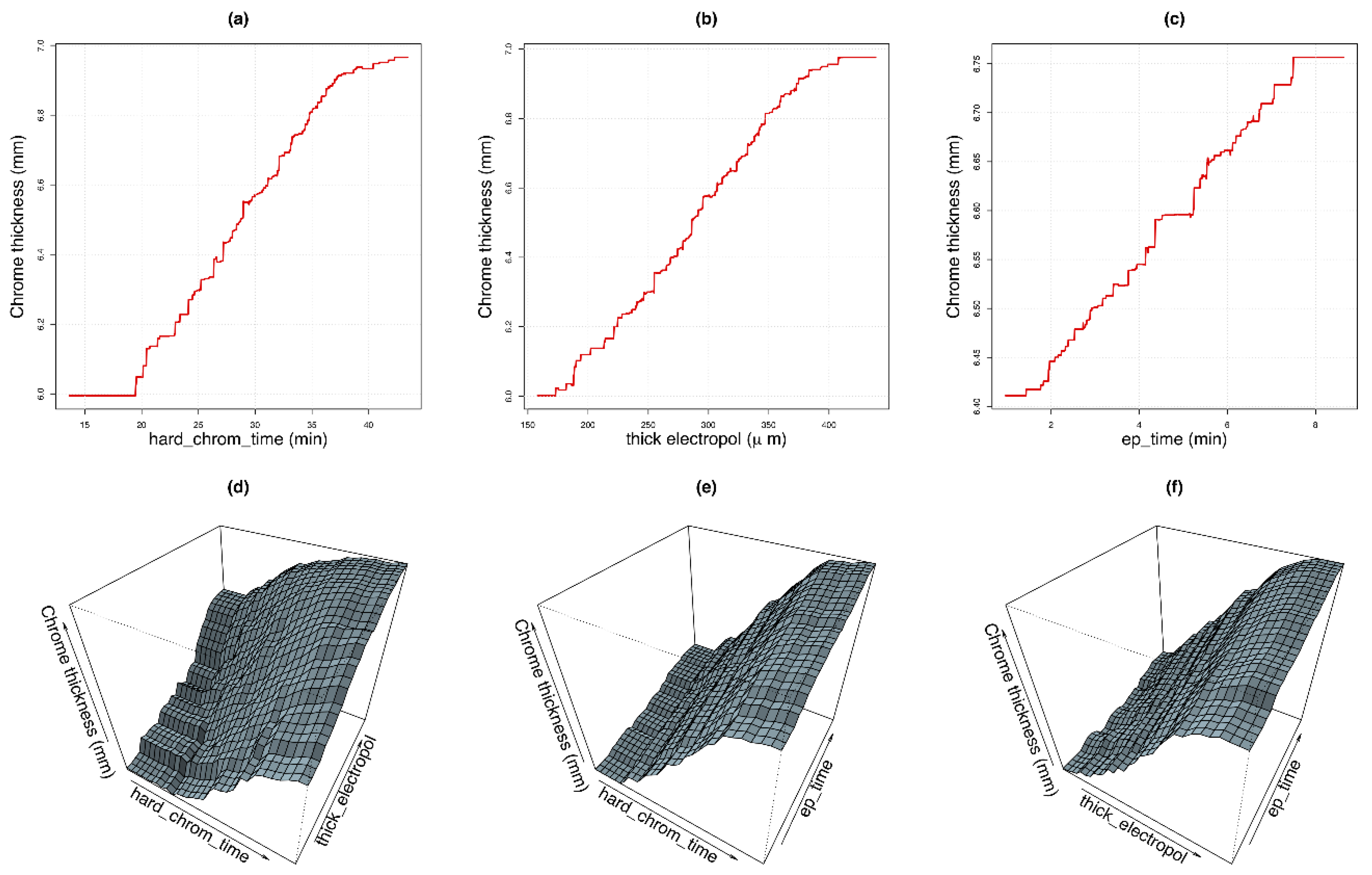
3. Results and Discussion

The derived hybrid model employed seven different input operator parameters as input variables. These were presented earlier in Table 1.

The hard chrome layer thickness was used as the output variable of the proposed novel hybrid DE/GBRT-based model. The prediction performed from the independent variables [14,15,16,17,18,19,33,35] was satisfactory. As previously stated, the GBRT technique is influenced by the selection of the GBRT hyperparameters, such as the learning rate, the maximum number of hyperparameters allowed, the amount of loss reduction, the minimum child weight, the maximum step, the and subsample ratio.

Parameter optimization was performed with the help of the differential evolution (DE) metaheuristic technique [22,23,24,25], which showed a good performance.

In this way, we constructed a hybrid model, namely the DE/GBRT-based model, which employs as the dependent variable the thickness of the hard chrome layer in the hard chromium plating process [10].

In order to study the effect of variables, the coefficient of determination was calculated. The flow chart of the model implemented in the present research is shown in Figure 5. The derivation of optimized hyperparameters follows an iterative process, where the model is created with a set of parameters and, then, its performance is obtained using the validation sets within the cross-validation process. According to the results obtained with previous sets, different sets of parameters are proposed by the DE algorithm and once the stopping condition is reached, the iteration ends.

Figure 6 shows those terms that are part of the best-fitted DE/GBRT-based model for the thickness of the hard chrome layer.

The graphical representation illustrates the importance of the variables involved in the model. As can be observed in the figure, the first line chart (see Figure 6a) corresponds to the thickness of the hard chrome layer (Y-axis) as a function of input variable hard chromium process time (X-axis). It can be observed that the built model shows that the chrome thickness increases with the processing time and electropolishing time, and grows with the material removed, which is in line with the actual process.

Figure 6d shows the variation of the thickness of the hard chrome layer as a function of hard chromium process time and the thickness of the layer removed by electropolishing, holding the remaining input variables constant. Here, it can be observed that the relative importance of the first two independent variables in the process is similar, as the chrome thickness grows at a similar rate with these two variables. Figure 6e,f show that electropolishing time has less influence over the process than the two previous independent variables, as chrome thickness remains relatively constant when this variable increases compared with the increment when the two other variables increase. This is consistent with the results shown in Figure 7, which show the relative importance of the variables within the model. The first two variables have similar importance while the third variable is less relevant.

The dataset was split into two sets: 70% of the data for the training set and the remainder of the data, 30%, for the testing set. R² was optimized with the help of the K–fold cross-validating methodology of [44] over the training set. The mean of the R² values obtained was considered to be the cross-validating R².

Table 2. Search space for each of the GBRT parameters in the DE tuning process and optimal hyperparameters of the best fitted GBRT model found with the DE technique.

GBRT Hyperparameters	Lower Limit	Upper Limit	Optimal Values
Rounds	1	100	99
$\eta$	0.1	1	0.12
$\gamma$	0	30	0.00004
Minimum child weight (MCW)	1	30	8.1
Maximum $\Delta$ step (MDS)	0	30	12
Subsample ratio	0.5	1	0.54

shows the intervals of the space of solutions used for the DE technique.

Therefore, the DE module was used to optimize the GBRT parameters using the comparison of the cross-validation error in each interaction. The search space has six dimensions and the points in Table 2 indicate the optimal hyperparameters of the best fitted DE/GBRT-based model found with the DE optimization technique.

Moreover,

Table 3. RMSE, coefficient of determination (R²) and correlation coefficient (r) for the hybrid DE/GBRT-based model fitted in this study for the thickness of the hard chrome layer using the testing data.

Model	RMSE	Coef. of Determination (R2)/Correlation Coef. (r)
DE/GBRT	0.01590	0.9842/0.9920

shows the RMSE, and the determination and correlation coefficients for the hybrid DE/GBRT-based model fitted for the thickness of the hard chromium layer in this manuscript.

Taking into account the results achieved, the GBRT technique in combination with DE optimization is suitable for building models with high performance for the estimation of the thickness of the hard chromium layer. The R² of the fitted GBRT model was 0.9842, with a correlation coefficient of 0.9920 and a RMSE of 0.01590.

The relevance measures are arguable and the sum of all the values for each criterion is equivalent to one. These criteria are:

• Gain: calculated by taking into account each variable contribution to each tree that makes up the model.
• Cover: defined as the relative number of the variable observations in the model.
• Frequency: the relative number of times that an independent variable materializes in the trees of the obtained model.

The most meaningful criterion is Frequency; therefore, it was utilized to contruct the chart of the relative relevance of the variables. According to the previous methodology, hard chromium process time is the most influential variable in the thickness of hard chromium layer prediction. This is consistent with the actual process, where the processing time is the main parameter of the operation. It is followed by the input variable layer thickness removed by electropolishing. Moreover, both the iron content of the electropolishing bath and electropolishing time are the third and fourth most influential variables in the thickness of hard chromium layer prediction, respectively. The fifth position in the influence ranking is held by the chromic acid content and the final positions are taken by electropolishing bath temperature and hard chrome bath temperature (see

Table 4. Significance ranking of the variables involved in the best fitted DE–GBRT-based model for the thickness of the hard chrome layer forecasting according to the criteria Gain, Cover and Frequency.

Input Variable	Gain	Cover	Frequency
hard_chrom_time	0.443652641	0.23208073	0.20448598
thick_electropol	0.424232729	0.26216224	0.22018692
iron_ep	0.047510359	0.09838727	0.14186916
ep_time	0.034522612	0.11615156	0.12953271
chrom_acid	0.031742450	0.10495429	0.12355140
ep_temp	0.009358148	0.09349104	0.09252336
hard_chrom_temp	0.008981060	0.09277288	0.08785047

and Figure 7).

Moreover, the model illustrated its capacity to predict the thickness of the hard chrome layer. Figure 8 indicates the comparison between the observed and predicted values of the thickness of the hard chrome layer using this hybrid DE/GBRT-based model. Thus, a suitable approach to tackle the issues associated with the nonlinearities of the problem is the utilization of a DE/GBRT–based model.

GBRT is able to process bigger datasets that other machine learning methods, such as SVR (support vector regression), MLPs (multilayer perceptrons) or ANNs (artificial neural networks), and provides more accurate results than methods such as MARS (multi-adaptative regression splines) or linear regression. Furthermore, DE needs fewer evaluations of the function than similar methods, such as PSO (particle swarm optimization) or ABC (artificial bee colony), which, in cases such as this, where many samples are processed, represent a bottleneck of the hyperparameter tuning process. Thus, the combination of DE and GBRT is an efficient procedure to predict the thickness of the hard chrome layer.

In summary, this study has permitted the estimation of the thickness of the hard chrome layer in concordance with real experimental values utilizing the DE/GBRT-based model with excellent precision and success. Hence, this work provides a convenient utilization of a GBRT model with a DE-based optimization method for the purpose of accomplishing the best effective approximation in the examined regression problem. Based on the ‘goodness of fit’ criteria (R² and RMSE), the results clearly show that the DE–GBRT-based model provides an excellent fit to actual data.

4. Conclusions

From the numerical and experimental results, the principal findings of this study are given as follows:

• A DE/GBRT-based model is an accurate tool for the purpose of estimating the thickness of the hard chrome layer.
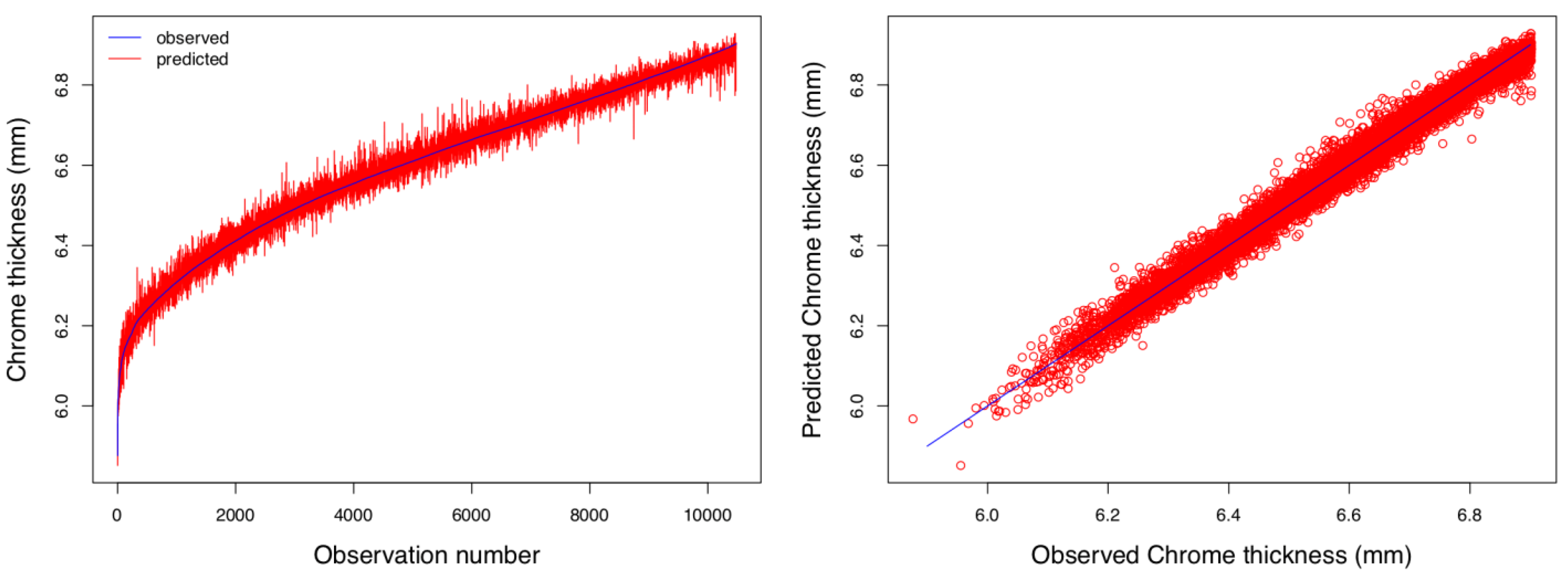
• In this research, we were able to predict the thickness of a hard-chrome layer from the measured independent variables. This kind of model is useful for industry in order to reduce the set-up costs of new industrial processes. This prediction was made with a RMSE of 0.01590.
• The modelled values were in concordance with the observed data; by applying the derived DE/GBRT model, a coefficient of determination equal to 0.9882 was achieved.
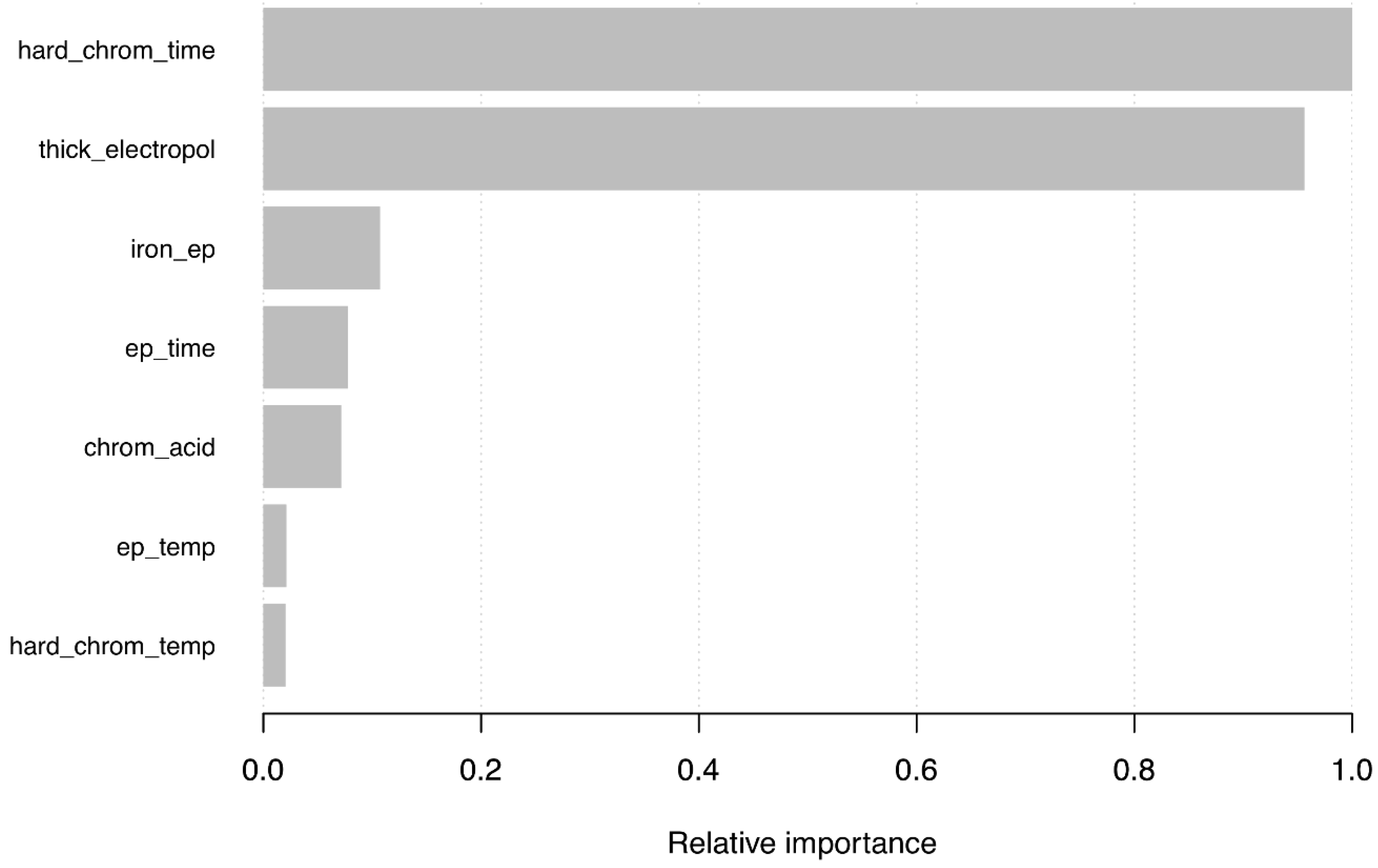
• Assessment of the importance of individual variables used in the process is possible. The order of importance of variables in the model for the determination of the thickness of the chromium layer was as follows: time of the hard chromium plating process measured in minutes, thickness of the layer removed by electropolishing in microns, iron content of the electropolishing bath in mg/L, electropolishing time in minutes, chromic acid content in g/L, electropolishing time in minutes and temperature of the hard chrome bath in degrees Celsius.
• The DE/GBRT-based model used the XGBoost algorithm [35,36,39] in combination with the DE optimization technique [23,39,40,41,42,43,44,45]. XGBoost is also termed the regularized boosting technique as its implementation involves regularization and, thus, is helpful in order to reduce overfitting.
• According to the results obtained, the DE/GBRT-based model was found to ameliorate the generalization ability by utilizing only the standard gradient boosted (GBM) regressor.

As a summary of the present study, it can be stated that this novel method can be applied to any similar plating process. In our opinion, this DE/GBRT-based model is an effective practical solution to the problem of the determination of the thickness of the hard chrome layer obtained by an industrial hard-chromium plating process.

References

1. Fink, C.G. Process of Electrodepositing Chromium and of Preparing Baths Therefor. U.S. Patent 1,581,188, 20 April 1926. [Google Scholar]
2. Dennis, J.K.; Such, T.E. The Nickel and Chromium Plating; Woodhead Publishing: New York, NY, USA, 1994. [Google Scholar]
3. Loffler, F. Methods to investigate mechanical properties of coatings. Thin Solid Films 1999, 339, 181–186. [Google Scholar] [CrossRef]
4. Yli-Pentti, A. Electroplating and Electroless Plating. Compr. Mater. Process. 2014, 13, 277–306. [Google Scholar]
5. Guffie, R.K. The Handbook of Chromium Plating; Gardner Publications Ltd.: New York, NY, USA, 1986. [Google Scholar]
6. Drozda, T.J.; Wick, C.; Mitchell, P.; Bakerjian, R.; Benedict, J.T.; Veilleux, R.F. Tool and Manufacturing Engineers Handbook: Materials Finishing and Coating; Society of Manufacturing Engineers: Dearborn, MI, USA, 1983. [Google Scholar]
7. Yin, K.-M.; Wang, C.M. A study on the deposit uniformity of hard chromium plating on the interior of small-diameter tubes. Surf. Coat. Technol. 1999, 144, 213–223. [Google Scholar] [CrossRef]
8. Khani, H.; Brennecke, J.F. Hard chromium composite electroplating on high-strength stainless steel from a Cr (III)-ionic liquid solution. Electrochem. Commun. 2019, 107, 106537. [Google Scholar] [CrossRef]
9. Davis, J.R. Surface Hardening of Steels: Understanding the Basics; ASM International: Columbus, OH, USA, 2002. [Google Scholar]
10. Lindsay, J.H. Decorative and hard chromium plating. Plat. Surf. Finish. 2003, 90, 22–24. [Google Scholar]
11. Iglesias García, C.; Sáiz Martinez, P.; García-Portilla González, M.P.; Bousoño García, M.; Jiménez Treviño, L.; Sánchez Lasheras, F.; Bobes, J. Effects of the economic crisis on demand due to mental disorders in Asturias: Data from the Asturias Cumulative Psychiatric Case Register. Actas Esp. Psiquiatr. 2014, 42, 108–115. [Google Scholar]
12. Schlesinger, M.; Paunovich, M. Modern Electroplating; Wiley-Interscience: New York, NY, USA, 2000. [Google Scholar]
13. Irving, B.; Knight, R.; Smith, R.W. The HVOF process—The hottest topic in the thermal spray industry. Weld. J. 1993, 72, 25–30. [Google Scholar]
14. Breiman, L.; Friedman, J.H.; Olshen, R.A.; Ston, C.J. Classification and Regression Trees; Wadsworth and Brooks/Cole: Monterey, CA, USA, 1984. [Google Scholar]
15. Vapnik, V. Statistical Learning Theory; Wiley-Interscience: New York, NY, USA, 1998. [Google Scholar]
16. Friedman, J.H. Stochastic gradient boosting. Comput. Stat. Data Anal. 2002, 38, 367–378. [Google Scholar] [CrossRef]
17. Schapire, R.E. The boosting approach to machine learning an overview. In Nonlinear Estimation and Classification; Denison, D.D., Hansen, M.H., Holmes, C.C., Mallick, B., Yu, B., Eds.; Lecture Notes in Statistics; Springer: Berlin, Germany, 2003; pp. 149–171. [Google Scholar]
18. Bühlmann, P.; Hothorn, T. Boosting algorithms: Regularization, prediction and model fitting. Stat. Sci. 2007, 22, 477–505. [Google Scholar] [CrossRef]
19. Hastie, T.; Tibshirani, R.; Friedman, J.H. The Elements of Statistical Learning; Springer-Verlag: New York, NY, USA, 2009. [Google Scholar]
20. Persson, C.; Bacher, P.; Shiga, T.; Madsen, H. Multi-site solar power forecasting using gradient boosted regression trees. Sol. Energy 2017, 150, 423–436. [Google Scholar] [CrossRef]
21. Johnson, N.E.; Ianiuk, O.; Cazap, D.; Liu, L.; Starobin, D.; Dobler, G.; Ghandehari, M. Patters of waste generation: A gradient boosting model for short-term waste prediction in New York City. Waste Manag. 2017, 62, 3–11. [Google Scholar] [CrossRef] [PubMed]
22. Storn, R.M.; Price, K. Differential evolution—A simple and efficient heuristic for global optimization over continuous spaces. J. Glob. Optim. 1997, 11, 341–359. [Google Scholar] [CrossRef]
23. Price, K.; Storn, R.M.; Lampinen, J.A. Differential Evolution: A Practical Approach to Global Optimization; Springer: Berlin, Germany, 2005. [Google Scholar]
24. Simon, D. Evolutionary Optimization Algorithms; Wiley: New York, NY, USA, 2013. [Google Scholar]
25. Yang, X.-S.; Cui, Z.; Xiao, R.; Gandomi, A.H.; Karamanoglu, M. Swarm Intelligence and Bio-inspired Computation: Theory and Applications; Elsevier: London, UK, 2013. [Google Scholar]
26. Uzal, E.; Moulder, J.C.; Rose, J.H. Experimental determination of the near-surface conductivity profiles of metal from electromagnetic induction (eddy current) measurement. Inverse Prob. 1994, 10, 753–764. [Google Scholar] [CrossRef]
27. Versaci, M. Fuzzy approach and Eddy currents NDT/NDE devices in industrial applications. Electron. Lett. 2016, 52, 943–945. [Google Scholar] [CrossRef]
28. Burrascano, P.; Callegari, S.; Montisci, A.; Ricci, M.; Versaci, M. (Eds.) Ultrasonic Nondestructive Evaluation Systems; Springer: Heidelberg, Germany, 2015. [Google Scholar]
29. Tanthadiloke, S.; Kittisupakorn, P.; Mujtaba, I.M. Modelling and Design a Controller for Improving the Plating Performance of a Hard Chromium Electroplating Process. In Proceedings of the 24th European Symposium on Computer Aided Process Engineering, Amsterdam, The Netherlands, 26 June 2018; Elsevier: Amsterdam, The Netherlands, 2014; pp. 805–810. [Google Scholar]
30. Sánchez Lasheras, F.; Vilán Vilán, J.A.; García Nieto, P.J.; del Coz Díaz, J.J. The use of design of experiments to improve a neural network model in order to predict the thickness of the chromium layer in a hard chromium plating process. Math. Comput. Model. 2014, 52, 1169–1176. [Google Scholar] [CrossRef]
31. Sánchez Lasheras, F.; García Nieto, P.J.; de Cos Juez, F.J.; Vilán Vilán, J.A. Evolutionary support vector regression algorithm applied to the prediction of the thickness of the chromium layer in a hard chromium plating process. Appl. Math. Comput. 2014, 227, 164–170. [Google Scholar] [CrossRef]
32. Friedman, J.H.; Hastie, T.; Tibshirani, R. Additive logistic regression: A statistical view of boosting. Ann. Stat. 2000, 28, 337–407. [Google Scholar] [CrossRef]
33. Friedman, J.H. Greedy function approximation: A gradient boosting machine. Ann. Stat. 2001, 29, 1189–1232. [Google Scholar] [CrossRef]
34. Taieb, S.B.; Hyndman, R.J. A gradient boosting approach to the kaggle load forecasting competition. Int. J. Forecast. 2014, 30, 382–394. [Google Scholar] [CrossRef] [Green Version]
35. Döpke, J.; Fritsche, U.; Pierdzioch, C. Predicting recessions with boosted regression trees. Int. J. Forecast. 2017, 33, 745–759. [Google Scholar] [CrossRef]
36. Ridgeway, G. Generalized Boosted Models: A Guide to the GBM. Available online: http://www.saedsayad.com/docs/gbm2.pdf (accessed on 3 August 2007).
37. Chen, T.; Guestrin, C. XGBoost: A Scalable Tree Boosting System. In Proceedings of the 22nd ACM SIGKDD International Conference on Knowledge Discovery and Data Mining, San Francisco, CA, USA, 13 August 2016; pp. 785–794. [Google Scholar]
38. Chen, T.; He, T.; Benesty, M.; Khotilovich, V.; Tang, Y. Xgboost: Extreme Gradient Boosting, R package, version 0.6-4; R Foundation for Statistical Computing: Vienna, Austria, 2017. Available online: https://CRAN.R-project.org/package=xgboost (accessed on 1 August 2019).
39. Feoktistov, V. Differential Evolution: In Search of Solutions; Springer: New York, NY, USA, 2006. [Google Scholar]
40. Rocca, P.; Oliveri, G.; Massa, A. Differential evolution as applied to electromagnetics. IEEE Trans. Antenn. Propag. 2011, 53, 38–49. [Google Scholar] [CrossRef]
41. Ridgeway, G. Gbm: Generalized Boosted Regression Models, R package, version 2.1.1; R Foundation for Statistical Computing: Vienna, Austria. Available online: http://CRAN.R-project.org/package=gbm (accessed on 21 March 2017).
42. Ardia, D.; Mullen, K.M.; Peterson, B.G.; Ulrich, J. DEoptim: Differential Evolution in R; R Package, Version 2.2-4; R Foundation for Statistical Computing: Vienna, Austria, 2016. [Google Scholar]
43. Freedman, D.; Pisani, R.; Purves, R. Statistics; WW Norton & Company: New York, NY, USA, 2007. [Google Scholar]
44. Picard, R.; Cook, D. Cross-validation of regression models. J. Am. Stat. Assoc. 1984, 79, 575–583. [Google Scholar] [CrossRef]
45. De Cos Juez, F.J.; Sánchez Lasheras, F.; García Nieto, P.J.; Álvarez-Arenal, A. Non-linear numerical analysis of a double-threaded titanium alloy dental implant by FEM. Appl. Math. Comput. 2008, 206, 952–967. [Google Scholar] [CrossRef]
Figure 1. Flowchart of the different stages of the industrial hard chromium plating process.
Mathematics 08 00959 g001
Figure 2. Tank for degreasing in the vapor phase.
Mathematics 08 00959 g002
Figure 3. Graphical overview of the process variables: variable value versus observation number.
Mathematics 08 00959 g003
Figure 4. Correlation matrix.
Mathematics 08 00959 g004
Figure 5. Flowchart of the new hybrid differential evolution/gradient boosted regression tree (DE/GBRT)-based model.
Mathematics 08 00959 g005
Figure 6. Graphical representation of the terms that constitute the hybrid DE/GBRT model for the thickness of the hard chromium layer: (a) hard chromium process time first-order term; (b) layer thickness removed by electropolishing first-order term; (c) electropolishing time first-order term; (d) hard chromium process time and layer thickness removed by electropolishing second-order term; (e) hard chromium process time and electropolishing time second-order term; and (f) layer thickness removed by electropolishing and electropolishing time.
Mathematics 08 00959 g006
Figure 7. Relative importance of the input operation variables to predict the thickness of the hard chromium layer.
Mathematics 08 00959 g007
Figure 8. Comparison between the chrome thickness values observed and predicted using the DE/GBRT-based model (RMSE = 0.0159 and R2 = 0.9842).
Mathematics 08 00959 g008