A Genetic Algorithm Optimized RNN-LSTM Model for Remaining Useful Life Prediction of Turbofan Engine

Abstract

Understanding the remaining useful life (RUL) of equipment is crucial for optimal predictive maintenance (PdM). This addresses the issues of equipment downtime and unnecessary maintenance checks in run-to-failure maintenance and preventive maintenance. Both feature extraction and prediction algorithm have played crucial roles on the performance of RUL prediction models. A benchmark dataset, namely Turbofan Engine Degradation Simulation Dataset, was selected for performance analysis and evaluation. The proposal of the combination of complete ensemble empirical mode decomposition and wavelet packet transform for feature extraction could reduce the average root-mean-square error (RMSE) by 5.14–27.15% compared with six approaches. When it comes to the prediction algorithm, the results of the RUL prediction model could be that the equipment needs to be repaired or replaced within a shorter or a longer period of time. Incorporating this characteristic could enhance the performance of the RUL prediction model. In this paper, we have proposed the RUL prediction algorithm in combination with recurrent neural network (RNN) and long short-term memory (LSTM). The former takes the advantages of short-term prediction whereas the latter manages better in long-term prediction. The weights to combine RNN and LSTM were designed by non-dominated sorting genetic algorithm II (NSGA-II). It achieved average RMSE of 17.2. It improved the RMSE by 6.07–14.72% compared with baseline models, stand-alone RNN, and stand-alone LSTM. Compared with existing works, the RMSE improvement by proposed work is 12.95–39.32%.

1. Introduction

Maintenance management has long been a core part of business management. It aims at maximizing functionality and minimizing breakdowns. Traditional run-to-failure maintenance and preventive maintenance become infeasible for meeting the smart maintenance perspective [1]. Run-to-failure maintenance schedules only when the equipment becomes malfunction. Preventive maintenance schedules regular maintenance to examine the status of equipment. With the advent of Internet of things (IoT) [2,3], sensors have been attached to equipment for continuous monitoring. Further data analytics via artificial intelligence (AI) techniques will provide valuable insights for better maintenance management. Using the solid foundation of IoT architecture, predictive maintenance (PdM) has started to replace traditional maintenance approaches. Different from traditional run-to-failure maintenance and preventive maintenance, predictive maintenance helps businesses to plan maintenance of equipment right before equipment failure. It is optimized between the preventive maintenance and run-to-failure. Predictive maintenance reduces the unnecessary maintenance check as in preventive maintenance. There are various successful stories in literature, summarized in the review articles [4,5].

The Airline Maintenance Cost Executive Commentary Edition 2019 reported the annual maintenance, repair, and overhaul cost was 9% ($69 billion) of the total operational cost [6]. In recent years, many remaining useful life (RUL) prediction algorithms [7,8,9,10,11,12,13,14,15,16] have been proposed to estimate the time of failure for turbofan engine. Thus, optimal PdM can be scheduled to reduce the maintenance cost and avoid equipment downtime.

In Section 1.1, the methodologies and performance of existing works of RUL prediction algorithms for turbofan engine are summarized. The limitations of existing works and motivations of our work are followed in Section 1.2. The research contributions of this paper are explained in Section 1.3.

1.1. Related Works

The RUL prediction algorithms can be categorized into shallow learning-based [7,8,9,10,11] and deep learning-based approaches [12,13,14,15,16]. Deep learning has become a preferred choice when performance of prediction model is outstanding compared with computational power. In the following, for fair and consistent comparison, all existing works are related to the RUL prediction of turbofan engine using identical benchmark dataset [17,18]. A brief summary on the methodology of related works [7,8,9,10,11,12,13,14,15,16] is presented. A detailed discussion and comparison between proposed work and related works will be shared in Section 3.4.

Shallow learning-based approaches are firstly summarized. In Mosallam et al. [7], a hybrid discrete Bayesian filter and k-nearest neighbors approach was proposed. It achieved average root-mean-square error (RMSE) of 27.57. Another work proposed a median distance to the k-nearest neighbors-based transfer learning approach for feature extraction [8]. It was then applied to random forest regression model. Results revealed that the average RMSE was 26. Zhao et al. [9] proposed a back propagation neural network as preliminary study of RUL prediction which yielded average RMSE of 42.6. An auto-regressive integrated moving average-based support vector regression was proposed in Ordóñez et al. [10]. Genetic algorithm (GA) was applied to fine-tune the parameters of the regression model. The performance had an average RMSE of 47.63. Apart from traditional machine learning algorithms, an innovative approach incorporated maximum Rao–Blackwellized particle filter, kernel two sample test, and maximum mean discrepancy was proposed by Cai et al. [11]. The average RMSE was 18.2.

Attention is drawn to deep learning-based approaches. It can be seen from the literature that a significant portion of articles adopted long short-term memory (LSTM). Researchers appreciated the effectiveness of LSTM in long-term prediction. A GA optimized restricted Boltzmann machine-based two layers LSTM model was proposed in Ellefsen et al. [12]. It obtained an average RMSE of 19.8. Adam adaptive learning rate optimization algorithm with single layer Vanilla LSTM model was applied and achieved average RMSE of 28.4 [13]. Likewise, Adam adaptive learning rate optimization algorithm was applied to optimize LSTM model in Wu et al. [14]. Evaluation showed that optimal performance (average RMSE of 19.1) was achieved for the setting of 5 layers and 100 neurons per layer. Other deep learning approaches were autoencoder gated recurrent unit [15] and deep convolution neural networks [16] which achieved average RMSE of 20.07 and 19.9, respectively.

In general, RUL prediction models using deep learning approaches outperform shallow learning-based approaches as the problem can be learnt more effectively via multiple layers architecture. It is agreed that shallow learning-based approaches offer low training time and light-weight models, however, computing power becomes a less important concern in today’s digital era. A reduction in average RMSE of prediction model outweighs the computing power. Particularly, the requirement of computing power in RUL prediction of turbofan engine is not exhaustive compared with image-based applications.

1.2. Research Gaps and Motivations

As mentioned before, both shallow learning-based [7,8,9,10,11] and deep learning-based algorithms [12,13,14,15,16] were applied for the RUL prediction of turbofan engine. Nevertheless, there is room for improvement in the following issues.

• Cross-validation was omitted in some studies [9,10,11,14,16] which may create a bias interpretation for the performance of model. For instance, certain training and testing datasets could be selected to produce smaller RMSE. In addition, some of the data may not be tested and thus lowering the generalization and robustness of model.
• There exist random failures over the life of the turbofan engine which existing algorithms [7,8,9,10,11,12,13,14,15,16] could not provide favorable performance for both short-term and long-term RUL prediction.
• Although deep learning-based approaches [12,13,14,15,16] achieved smaller RMSE compared with shallow learning-based approaches [7,8,9,10,11], there is room for improvement to further reduce the RMSE.

To address these limitations, we have the following point-to-point considerations.

• A 10-fold cross-validation is adopted for performance evaluation of RUL prediction model.
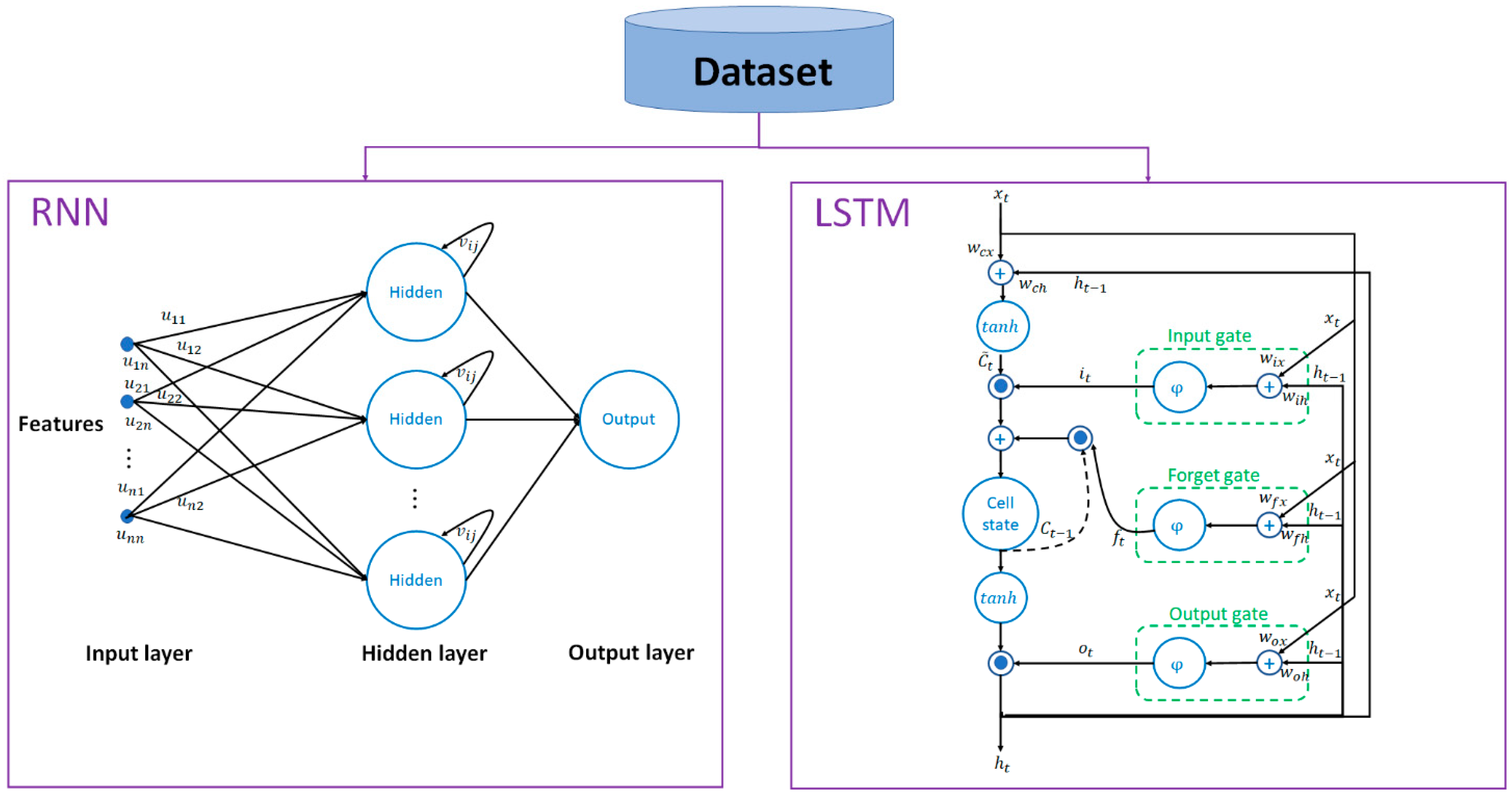
• We combine recurrent neural network (RNN) and LSTM which take the advantages in managing both short-term and long-term RUL predictions.
• NSGA-II is adopted to optimally design the RNN-LSTM model.

1.3. Research Contributions

The research contributions of this paper are summarized as follows.

• The combined model RNN-LSTM takes the advantages in RUL prediction of turbofan engine under short-term and long-term conditions. Results reveal that it reduces RMSE by 6.07–14.72% compared with stand-alone RNN and stand-alone LSTM.
• The combination of complete ensemble empirical mode decomposition (CEEMD) and wavelet packet transform (WPT) as two-step decomposition for feature extraction takes the advantages in capturing both time and frequency information. It reduces the RMSE by 5.14–27.15% compared with CEEMD, EEMD, EMD, WPT, EEMD-WPT, and EMD-WPT.
• Non-dominated sorting genetic algorithm II (NSGA-II) optimally designs the RNN-LSTM for optimal performance on short-term and long-term predictions.
• The proposed NSGA-II optimized RNN-LSTM model outperformed related works by 12.95–39.32% in terms of RMSE.

2. Methodology of Proposed NSGA-II Optimized RNN-LSTM Model

This section is organized as follows. Figure 1 shows the system overview of the proposed NSGA-II optimized RNN-LSTM model via CEEMD-WPT for feature extraction. The feature extraction is firstly discussed. This is followed by the NSGA-II optimized RNN-LSTM model.

2.1. Feature Extraction

Features are extracted based on the combination of complete ensemble empirical mode decomposition (CEEMD) and wavelet packet transform (WPT) namely CEEMD-WPT. The rationale behind the combination is as follows.

Compared with empirical mode decomposition (EMD) and ensemble empirical mode decomposition (EEMD), CEEMD reduces the residual noise and thus achieves smaller reconstruction error [19,20]. Furthermore, the requirement of computational power is lowered. In general, CEEMD decomposes the nonlinear turbofan engine signals into intrinsic mode functions (IMFs) and a residual. It captures the frequency and temporal resolutions of the signals. The next step is to further decompose the IMFs as detail and approximation coefficients using WPT. It is noted that WPT takes the advantages in retaining the localization properties, smoothness, and orthogonality [21,22]. Therefore, the proposal of hybrid CEEMD-WPT takes the advantage in capturing both time and frequency information. Particularly, this is two-step decomposition.

The mathematical formulations of merging traditional CEEMD and WPT as CEEMD-WPT are illustrated as follows.

Assume dataset $X=\left[x\left(1\right),\dots ,x\left(N\right)\right]\in R^N$ which is decomposed into IMFs and a residual using CEEMD. Assume the signal is merged with Gaussian noises $N\left(0,1\right)$ (realization $i=1,\dots ,L$) on each residual $r_j$. The first IMF ${\widetilde{IMF}}_1\left(t\right)$ and residual $r_1\left(t\right)$ can be obtained using Equations (1)–(4).

$${\overline{x}}^i\left(t\right)=x\left(t\right)+{\sigma }_0{w}^i\left(t\right),t\in 1,\dots ,N$$

(1)

$$IM{F}_1^i\left(t\right)=EM{D}_1\left({\overline{x}}^i\left(t\right)\right)$$

(2)

$${\widetilde{IMF}}_1\left(t\right)=\frac{1}{L}{\displaystyle \sum }_{i=1}^{L}IM{F}_1^i\left(t\right)$$

(3)

$$r_1\left(t\right)=x\left(t\right)-{\widetilde{IMF}}_1\left(t\right)$$

(4)

where ${\overline{x}}^i\left(t\right)$ is the temporary signal of original signal $x\left(t\right)$ masked by Gaussian noise $w^i\left(t\right)$ with noise standard deviation ${\sigma }_0$, and $EMD\left(·\right)$ denotes the fundamental EMD function.

Equations (5)–(7) are repeated until ${\overline{r}}_j\left(t\right)$ has only one extreme, which cannot be further decomposed.

$${\overline{r}}_j^i\left(t\right)=r_j\left(t\right)+{\sigma }_j{w}^i\left(t\right)$$

(5)

$${\widetilde{IMF}}_j\left(t\right)=\frac{1}{L}{\displaystyle \sum }_{i=1}^{L}EM{D}_1\left({\overline{r}}_{j-1}\left(t\right)\right)$$

(6)

$$r_j\left(t\right)=r_{j-1}\left(t\right)-{\widetilde{IMF}}_{j-1}\left(t\right)$$

(7)

The final residual can be calculated using:

$$r_{final}\left(t\right)=x\left(t\right)-{\displaystyle \sum }_{j=1}^J{\widetilde{IMF}}_j\left(t\right)$$

(8)

where $j=1,\dots ,J$. The original signal can be reconstructed by rearranging Equation (8):

$$x\left(t\right)={\displaystyle \sum }_{j=1}^J{\widetilde{IMF}}_j\left(t\right)+r_{final}\left(t\right)$$

(9)

WPT further decomposes each of the ${\widetilde{IMF}}_j\left(t\right)$ of length L into extended version ${\widetilde{IMF}}_j{\left(t\right)}_{ext}=\left[{\widetilde{IMF}}_{j,0},{\widetilde{IMF}}_{j,1},\dots ,{\widetilde{IMF}}_{j,L_x}\right]$ into mother wavelet. Denote L_x as the length of extended ${\widetilde{IMF}}_j\left(t\right)$, which is given by:

$$L_x=\{\begin{array}{c}L+2\left(M-2\right)+0\\ L+2\left(M-2\right)+1\end{array}\begin{array}{c}evenL\\ oddL\end{array}$$

(10)

where M is the number of low-pass filter coefficients with low-pass filter $h_{low}$ defined as:

$$h_{low}=\left[h_{low,0},h_{low,1},\dots ,h_{low,M-1}\right]$$

(11)

The approximation coefficients of WPT on ${\widetilde{IMF}}_j\left(t\right)$ with $h_{low}$ is given by:

$$\begin{array}{c}C{L}_{j,0}={\widetilde{IMF}}_{j,0}\times h_{low,0}+{\widetilde{IMF}}_{j,1}\times h_{low,1}+\cdots +{\widetilde{IMF}}_{j,M-1}\times h_{low,M-1}\\ C{L}_{j,1}={\widetilde{IMF}}_{j,2}\times h_{low,0}+{\widetilde{IMF}}_{j,3}\times h_{low,1}+\cdots +{\widetilde{IMF}}_{j,M+1}\times h_{low,M-1}\\ ⋮\\ C{L}_{j,\left(\left(L_x-M\right)/2\right)}={\widetilde{IMF}}_{j,L_x-M}\times h_{low,0}+{\widetilde{IMF}}_{j,L_x-M+1}\times h_{low,1}+\cdots +{\widetilde{IMF}}_{j,L_x-1}\times h_{low,M-1}\end{array}$$

(12)

For simplicity, we may rewrite Equation (12) as:

$$C{L}_{j,k}={{\displaystyle \sum }}_{l=0}^{M-1}{\widetilde{IMF}}_{j,2\ast k+l}\times h_{low,l}\forall k\left[0,\left(L_x-M\right)/2\right]$$

(13)

Define the high-pass filter $h_{high}$ of length M as follows:

$$h_{high}=\left[h_{high,0},h_{high,1},\dots ,h_{high,M-1}\right]$$

(14)

The approximation coefficients of WPT on ${\widetilde{IMF}}_j\left(t\right)$ with $h_{high}$ is given by:

$$\begin{array}{c}C{H}_{j,0}={\widetilde{IMF}}_{j,0}\times h_{high,0}+{\widetilde{IMF}}_{j,1}\times h_{high,1}+\cdots +{\widetilde{IMF}}_{j,M-1}\times h_{high,M-1}\\ C{H}_{j,1}={\widetilde{IMF}}_{j,2}\times h_{high,0}+{\widetilde{IMF}}_{j,3}\times h_{high,1}+\cdots +{\widetilde{IMF}}_{j,M+1}\times h_{high,M-1}\\ ⋮\\ C{H}_{j,\left(\left(L_x-M\right)/2\right)}={\widetilde{IMF}}_{j,L_x-M}\times h_{high,0}+{\widetilde{IMF}}_{j,L_x-M+1}\times h_{high,1}+\cdots +{\widetilde{IMF}}_{j,L_x-1}\times h_{high,M-1}\end{array}$$

(15)

For simplicity, we may rewrite Equation (15) as:

$$C{H}_{j,k}={{\displaystyle \sum }}_{l=0}^{M-1}{\widetilde{IMF}}_{j,2\ast k+l}\times h_{high,l}\forall k\left[0,\left(L_x-M\right)/2\right]$$

(16)

In this article, we have chosen various types of wavelet for analysis, including Haar wavelet, Daubechies wavelet (D2, D4, D6, D8, and D10), and Coiflet (C1, C2, C3, C4, C5).

Figure 2 shows an example of CEEMD-WPT which includes the plots for IMF 1–6 and residue, as output of CEEMD, as well as approximation coefficients and detail coefficients as output of WPT.

Inspired by Plaza et al. [23] of WPT for vibration signals, we computed the statistical features namely Shannon entropy, kurtosis, skewness, peak-to-peak amplitude, standard deviation, and mean of the coefficients for feature construction.

2.2. NSGA-II Optimized RNN-LSTM Model

The stand-alone RNN and stand-alone LSTM models are firstly trained independently. This is followed by optimally designing the RNN-LSTM model via the introduction of weighting factors which will be solved by NSGA-II.

Figure 3 shows the architectures of the proposed RNN and LSTM model which will be illustrated in Section 2.2.1 and Section 2.2.2, respectively. NSGA-II will be applied to optimally design RNN-LSTM model in Section 2.2.3.

2.2.1. Formulation of RNN

The architecture of RNN relies on previous information (t − 1) to generate output of information for current time (t). A standard three-layer Elman network is employed. The input is fed forward to the hidden layer with learning. There is connection to retain the previous information of the hidden unit in the context unit. The formulation is given by:

$$h_t={\phi }_h\left(U_{in}{x}_t+V_h{h}_{t-1}+b_h\right)$$

(17)

$$y_t={\phi }_y\left(W_{out}{h}_t+b_y\right)$$

(18)

where $h_{t-1}$ and $h_t$ is the vector for the hidden layer at previous time and current time, respectively; ${\phi }_h$ and ${\phi }_y$ are the activation functions for the hidden layer and the output layer, respectively; $U_{in}$ is the weight matrix between the input and hidden layer; $V_{in}$ is the weight matrix between the hidden layers; $b_h$ and $b_y$ are vectors for biases in the hidden layer and output layer; $W_{out}$ is the weight matrix between the hidden layer and the output layer.

Traditional activation functions like sigmoid, tanh, and rectified linear unit (ReLU) may suffer from slow convergence speed and thus other nonlinear functions, power-sigmoid and bipolar-sigmoid activation functions have been utilized for RNN implementation [24,25]. The formulations are defined as:

• Power-sigmoid activation function:

  $$\phi \left(x\right)=\{\begin{array}{c}\frac{\left(1-e^{-\epsilon x}\right)\left(1+e^{-\epsilon }\right)}{\left(1-e^{-\epsilon }\right)\left(1+e^{-\epsilon x}\right)}\\ x^a\end{array}\begin{array}{c}\left|x\right|<1\\ \left|x\right|\ge 1\end{array}$$

  (19)

  where $\epsilon >2$ and $a\ge 3$.
• Bipolar-sigmoid activation function:

  $$\phi \left(x\right)=\frac{1-e^{-\epsilon x}}{1+e^{-\epsilon x}}$$

  (20)

  where $\epsilon >2$.

2.2.2. Formulation of LSTM

The LSTM network takes the advantage to address time series data because of the ability to map between input and output sequences with contextual information. The workflows of the forget gate, the input gate, and the output gate of LSTM network have been summarized as follows. Define $W_f$, $W_{in}$, $W_{out}$, and $W_c$ as the weight matrices of the forget gate, the input gate, the output gate, and the memory cell, respectively. The corresponding bias vectors are $b_f$, $b_{in}$, $b_{out}$, and $b_c$, respectively.

• Forget gate:
  The forget gate $f_t$ takes the latest input $x_t$ and previous output of memory block $h_{t-1}$. The activation function ${\phi }_a$ of the forget gate is chosen to be logistic sigmoid as common practice, determines how much information is reserved the upper cell.

  $$f_t={\phi }_a\left(W_f\times \left[h_{t-1},x_t\right]+b_f\right)$$

  (21)
• Input gate:
  The information flowing into the cell is controlled by the input gate $i_t$.

  $$i_t={\phi }_a\left(W_{in}\times \left[h_{t-1},x_t\right]+b_{in}\right)$$

  (22)
• Output gate:
  The output of the memory cell is regulated by the output gate $o_t$.

  $$o_t={\phi }_a\left(W_{out}\times \left[h_{t-1},x_t\right]+b_{out}\right)$$

  (23)
• Memory cell:
  A tanh layer creates a vector of new candidate values ${\tilde{C}}_t$ that could be added to the state.

  $${\tilde{C}}_t=tanh\left(W_c\times \left[h_{t-1},x_t\right]+b_c\right)$$

  (24)

  $$h_t=o_t\ast \tanh \left(C_t\right)$$

  (25)

The state of the old memory cell $C_{t-1}$ is updated to new memory cell $C_t$.

$$C_t=f_t\ast C_{t-1}+i_t\ast {\tilde{C}}_t$$

(26)

2.2.3. Optimal Design of RNN-LSTM Using NSGA-II

Each RNN model and LSTM model produces predictions namely ${\widehat{y}}_{RNN}$ and ${\widehat{y}}_{LSTM}$, respectively. We optimally join the models as RNN-LSTM by introducing weighting factors ${\omega }_{RNN}$ and ${\omega }_{LSTM}$. The predictions of RNN-LSTM become:

$${\widehat{y}}_{RNN-LSTM}={\omega }_{RNN}{\widehat{y}}_{RNN}+{\omega }_{LSTM}{\widehat{y}}_{LSTM}$$

(27)

NSGA-II is adopted to optimally design ${\omega }_{RNN}$ and ${\omega }_{LSTM}$ by setting the objective functions F1 as minimization of the RMSE and F2 as the minimization of the mean absolute error (MAE). The objective functions are defined in multidimensional space, also named as objective space. Crossover is the operation to combine genetic material of two or more solutions. Most species have two parents except some have one parent. In GA, it can be extended to more than two parents. N-point crossover is famous for bit string representation. Two solutions at n positions are spitted up and alternately assembled to a new one. For instance, assume one-point crossover between 001110010 and 1111010111. It randomly selects a position (let us say 4), the offspring candidate solutions can be 0010-010111 and 1111-110010. For continuous representations, numerical operations are utilized for the orientation of crossover operators. Arithmetic crossover is one of the popular operations that computes the arithmetic mean of all parental solutions component-wise. For example, two parents (3,8,5) and (2,6,4) will generate an offspring of (2.5,7,4.5).

The second operation of GA is mutation. It is based on random changes from which the solution is disturbed. The strength of disturbance is quantified by mutation rate (bit string representation) and step size (continuous representation). There are three design principles for mutation operators. The first principle is reachability. The arbitrary point in the solution space must be reachable to each point in the solution space. Adding constraints to the optimization problem can reduce the reachability in which the solution space becomes a feasible subset. Secondly, the unbiasedness principle prohibits the induction of drift of the search to any direction in unconstrained solution spaces. In the case of constrained solution space, bias may be allowed as advantageous. Scalability is the third design principle. Each mutation operator is adaptable to offer the degree of freedom. The probability distribution is usually adopted for mutation operators. Let uss consider Gaussian mutation using Gaussian distribution, the standard deviation can scale the samples in the entire solution space.

The quality of the phenotype of the solution is governed by the fitness function. The design of fitness function is an essential component of the algorithm. When it comes to the multi-objective optimization problem, the values of the fitness function of each single objective are summed. The fitness values of the individuals are ranked based on the values of the objective functions. The rationale behind the minimization of both RMSE and MAE is minimizing RMSE is equivalent to the prediction of the mean whereas minimizing MAE is equivalent to the prediction of median [26]. It is a well-known optimization algorithm which improves NSGA by introducing elite strategy, crowding degree, and fast non-dominated sorting technique [27,28,29]. The best offspring solutions are selected as parents in the new parental population. This aims at converging the solution to optimal solutions. The selection process is based on the fitness value in the population. As we are handling minimization problem, low fitness values are preferred.

In general, the multi-objective optimization problem aims at obtaining trade-off optimal solutions. There exist many possible solutions of ${\omega }_{RNN}$ and ${\omega }_{LSTM}$ with corresponding predicted value ${\widehat{y}}_{RNN-LSTM}$. The design of the weightings determines how the RUL prediction model characterizes the advantages of RNN and LSTM for short-term and long-term RUL prediction. To obtain the output, i.e., the optimal set of ${\omega }_{RNN}$ and ${\omega }_{LSTM}$, it requires high computing power. Therefore, a tradeoff between the computing power and convergence of RUL prediction model is expected.

Within the objective space, Pareto optimal solution is defined as the optimal solution whereas the Pareto front is defined as the set of Pareto optimal solutions. Attributed to the errors of stochastic selection in finite population, a small group of the Pareto optimal solutions (but not all the optimal solutions) determine the convergence of the population.

The algorithm of NSGA-II can be found in Algorithm 1.

Algorithm 1$\mathrm{Training}({\left\{X\right\}}_{train})$
Input: Training datasets ${\left\{X\right\}}_{train}$
Output: RUL Prediction Model
	1:  Initialize NSGA-II parameters including population size and values of objec-tive functions; 2:  Allocate non-dominated ranks for the individuals; 3:  while generations g <= max_generation do 4:  Perform the operations including selections, crossover, and mutation; 5:  Merge population (initial population and offspring) and allocate non-dominated ranks for the individuals in the merged population; 6:  Follow truncation mechanism that retains non-dominated solutions with higher crowding distance and maximum number of solutions is equal to the population size; 7:  Allocate non-dominated ranks for the individuals; 8:  Extract Pareto-optimal front; 9:  Determine the optimal solution based on the values of objective functions; and 10:  g = g + 1; 11:  End while 12:  Model←Pareto optimal solutions

3. Results

The benchmark dataset is firstly presented for the performance evaluation of RUL prediction model. Analysis was conducted based on (i) comparison between stand-alone RNN, stand-alone LSTM, and proposed NSGA-II optimized RNN-LSTM; (ii) Comparison feature extractions approaches EMD, EEMD, CEEMD, EMD-WPT, EEMD-WPT, with proposed CEEMD-WPT; and (iii) comparison between proposed NSGA-II optimized RNN-LSTM and existing works.

3.1. Commercial Modular Aero-Propulsion System Simulation Turbonfan Degradation (C-MAPSS-TD) Dataset

In the field of RUL prediction of turbofan engine, Commercial Modular Aero-Propulsion System Simulation Turbofan Degradation (C-MAPSS-TD) dataset is a well-known and benchmark dataset [17,18].

Table 1. Summary of Commercial Modular Aero-Propulsion System Simulation Turbofan Degradation (C-MAPSS-TD) dataset.

	Subset
	FD001	FD002	FD003	FD004
Number of engine units (Total)	200	519	200	497
Number of engine units (Training)	180 in 1st–10th folds	468 in 1st–9th folds and 459 in 10th folds	180 in 1st–10th folds	450 in 1st–7th folds and 441 in 10th folds
Number of engine units (Testing)	20 in 1st–10th folds	51 in 1st–9th folds and 60 in 10th folds	20 in 1st–10th folds	47 in 1st–7th folds and 56 in 8th–10th folds
Number of operating conditions	1	6	1	6
Number of fault modes	1	1	2	2

summarizes the information of the C-MAPSS-TD dataset including the total number of engine units (vary from 200 to 519), the number of engine units (training), the number of engine units (testing), the number of operating conditions (either 1 or 6), and the number of fault modes (either 1 or 2).

It is worth noting that the total number of engine units in FD002 and FD004 are not divisible by 10, the settings of training and testing datasets may not be identical in all folds. Each datum contains 26 columns covering engine identity (ID), timestamp, 3 operational settings, and 21 sensor measurements.

We have analyzed the performance of RUL prediction models in existing works [7,8,9,10,11,12,13,14,15,16] and suggested the level of difficulty among FD001–FD004. The ranks are given by FD004 > FD002 > FD003 > FD001. The level of difficulty increases with the increase in the number of operating conditions and the number of fault modes.

3.2. Comparison between Feature Extraction Approaches

In this paper, we have proposed CEEMD-WPT for feature extraction which is compared with single decomposition-based approaches EMD, EEMD, CEEMD, and WPT, as well as hybrid decomposition-based approaches EMD-WPT and EEMD-WPT.

Table 2. Performance evaluation of EMD, EEMD, CEEMD, WPT, EMD-WPT, EEMD-WPT, and proposed CEEMD-WPT.

	FD001	FD002	FD003	FD004
Method	RMSE/MAE
EMD	14.96/14.18	22.82/22.36	15.35/14.47	23.28/22.38
EEMD	14.53/13.71	22.35/21.83	14.92/13.91	22.89/22.05
CEEMD	14.29/13.37	22.27/21.42	14.68/13.78	22.44/21.84
WPT	15.36/14.32	23.53/22.61	15.63/14.77	23.69/22.83
EMD-WPT	12.82/11.67	20.98/19.69	13.01/12.02	20.73/20.13
EEMD-WPT	12.66/11.35	20.74/19.28	12.85/11.68	20.31/19.74
Proposed CEEMD-WPT	11.19/10.28	19.33/18.50	11.47/10.66	19.74/18.82

shares the RMSE and MAE of seven approaches in datasets FD001–FD004.

The proposed hybrid decomposition via CEEMD-WPT outperforms the other six methods in both RMSE and MAE. The range of percentage reductions in RMSE are 11.61–27.15%, 6.80–17.85%, 10.74–26.62%, and 5.14–17.37%, for FD001, FD002, FD003, and FD004, respectively. Likewise, for the percentage reductions in MAE, they are 9.43–28.21%, 4.05–18.18%, 8.73–27.83%, and 4.66–17.56%, respectively. Another observation is that hybrid decomposition, CEEMD-WPT, EEMD-WPT, and EMD-WPT achieve better performance compared with single decomposition, EMD, EEMD, CEEMD, and WPT.

3.3. Comparison between Stand-Alone RNN, Stand-Alone LSTM, and Proposed NSGA-II Optimized RNN-LSTM

To illustrate the results of RUL prediction problem, Figure 4 shows two examples of the predicted RUL and true RUL for engine unit numbers 5 and 82. It can be seen that the proposed NSGA-II optimized RNN-LSTM model takes the advantages in both short-term and long-term prediction which the deviations between true and predicted RUL can be reduced across the whole range of time (cycle).

To reveal the necessity of merging RNN and LSTM, i.e., the proposed NSGA-II optimized RNN-LSTM model, evaluation and comparison are made with the baseline models, stand-alone RNN, and the stand-alone LSTM models. For fair comparison, analysis is based on feature extraction using CEEMD-WPT. K-fold cross-validation is chosen as a common way of performance evaluation, in which K = 10 is adopted and supported by many real-world applications [30,31,32].

Table 3. Performance evaluation of stand-alone RNN, stand-alone LSTM, and proposed algorithm.

	FD001	FD002	FD003	FD004
Method	RMSE/MAE
Stand-alone RNN	13.08/11.74	21.77/20.71	13.45/12.06	21.87/20.93
Stand-alone LSTM	12.04/11.17	20.58/19.65	12.39/11.39	21.15/20.46
Proposed NSGA-II optimized RNN-LSTM	11.19/10.28	19.33/18.50	11.47/10.66	19.74/18.82

summarizes the RMSE and MAE of the three approaches in datasets FD001–FD004. The RMSE is based on the average of 10 results in 10-fold cross-validation.

Results in Table 3 reveal that the proposed NSGA-II optimized RNN-LSTM model outperforms (achieving lowest RMSE) stand-alone RNN model and stand-alone LSTM model. The ranks are given by Proposed > LSTM > RNN. The percentage reductions of RMSE by proposed method are (7.06,14.45), (6.07,11.21), (7.43,14.72), and (6.67,9.74), for FD001, FD002, FD003, and FD004, respectively. Likewise, the percentage reductions of MAE by proposed method are (7.97,12.44), (5.85,10.67), (6.41,11.61), and (8.02,10.08), respectively. Therefore, the RUL prediction model takes the advantages from RNN and LSTM with proposed method.

3.4. Comparison between Proposed Work and Existing Works

The proposed work was compared with shallow learning-based approaches [7,8,9,10,11] and deep learning-based approaches [12,13,14,15,16]. Methodology, cross-validation, and RMSE of each work have been summarized in

Table 4. Performance comparison between proposed work and existing works.

Work	Methodology	Cross-Validation	RMSE
			FD001	FD002	FD003	FD004
[7]	Hybrid discrete Bayesian filter and k-nearest neighbors	3-fold	27.57
[8]	k nearest neighbors-based transfer learning and random forest regression	4-fold	26
[9]	Back propagation neural network	No	42.6
[10]	Auto-regressive integrated moving average-based support vector regression	No	47.63
[11]	Maximum Rao–Blackwellized particle filter, kernel two sample test, and maximum mean discrepancy	No	15.94	17.15	16.17	20.72
			Average (18.2)
[12]	LSTM	10-fold	12.56	22.73	12.10	22.66
			Average (19.8)
[13]	Vanilla LSTM	5-fold	19.76	27.26	24.04	34.72
			Average (28.4)
[14]	Adam adaptive learning optimized LSTM	No	18.43	N/A	19.78	N/A
			Average (19.1)
[15]	Autoencoder gated recurrent unit	5-fold	20.07
[16]	Deep convolution neural networks	No	12.61	22.36	12.64	23.31
			Average (19.9)
Proposed	NSGA-II optimized RNN-LSTM	10-fold	11.19	19.33	11.47	19.74
			Average (17.2)

.

Both shallow learning [7,8,9,10,11] and deep learning [12,13,14,15,16] have been reported for RUL prediction in literature. Researchers may consider adopting shallow learning when they prefer models with lower requirement on computational power and faster research analysis, with fair model performance (e.g., RMSE in RUL prediction). On the other hand, deep learning approaches require larger computational power and may suffer from slower research analysis with smaller RMSE.

Since the performance of RUL prediction model using shallow learning may not yield favorable model performance, research works are usually built the prediction model with hybrid techniques, as in Mosallam et al. [7], Fan et al. [8], Ordóñez et al. [10], and Cai et al. [11]. The rationale behind this is to take advantages from different techniques to further enhance the performance because there is no one that method fits all applications. Likewise, for deep learning-based approaches, some works (Wu et al. [14] and proposed work) introduce hybrid techniques for RUL prediction.

The stability of the RUL prediction model can be examined. In general, a trained model must be tested by unseen data in order to confirm the effectiveness of the model when it is deployed. The trained model is expected to capture the characteristics from the data, without too much influence by noisy data. Technically speaking, the model should have low variance and bias. K-fold cross-validation is adopted. The higher the value of k, the less the bias is, nevertheless, the higher the variability is. In contrast, the lower the value of k, the more the bias is. Therefore, k = 10 is chosen as typical value which has been supported by various works [30,31,32].

In literature, some works [9,10,11,14,16] did not employ cross-validation in which the results are not convincing to reflect the model performance in practice. The others [7,8,12,13,15] and proposed work employed k-fold cross-validation (various possibilities of k = 3, k = 4, k = 5, and k = 10) for performance evaluation. Although the selection of the value of k may be different, comparison could be made between these works given k-fold cross-validation has been adopted.

For fair comparison, the proposed work compares with existing works [7,8,12,13,15] that have adopted k-fold cross-validation. Results reveal that the proposed work outperforms existing works in both overall RMSE and RMSE of individual dataset. The range of percentage improvements are 12.95–39.32%, 10.91–43.37%, 14.96–29.09%, 5.21–52.29%, and 12.89–43.15%, for overall RMSE, FD001, FD002, FD003, and FD004, respectively.

The reasons for the improvements by proposed work are two-fold: (i) the two-step decomposition via CEEMD-WPT captures both time and frequency information for feature extraction; and (ii) NSGA-II optimally merges the results of RNN and LSTM as RNN-LSTM which take advantages from RNN and LSTM for short-term and long-term predictions which reduce the prediction errors across all time (cycle).

4. Conclusions

Optimal predictive maintenance can be scheduled to reduce the maintenance cost and avoid equipment downtime. In this paper, an innovative NSGA-II optimized RNN-LSTM algorithm was proposed for RUL prediction of turbo fan engine. A hybrid decomposition CEEMD-WPT was introduced to enhance the feature extraction process. A benchmark C-MAPSS-TD dataset was chosen to evaluate the performance of proposed work. It achieved average RMSE and average MAE of 17.2 and 16.3, respectively for overall datasets FD001–FD004. To evaluate the effectiveness of hybrid decomposition CEEMD-WPT and RNN-LSTM, analysis was conducted. Results reveal that CEEMD-WPT reduces the RMSE by 5.14–27.15% using individual dataset FD001-FD004 compared with CEEMD, EEMD, EMD, WPT, EEMD-WPT, and EMD-WPT. Likewise, RNN-LSTM reduces RMSE by 6.07–14.72% compared with stand-alone RNN and stand-alone LSTM. Compared with existing works, the proposed work reduces the RMSE by 12.95–39.32%.

Although the proposed work has improved the RMSE, there is room for further improvement. It is suggested to generate more training data which helps enhancing the performance of deep learning model. Typical data generation methods include information maximizing generative adversarial network [33], conditional generative adversarial network [34], and auxiliary classifier generative adversarial network [35].

References

1. Bokrantz, J.; Skoogh, A.; Berlin, C.; Wuest, T.; Stahre, J. Smart maintenance: A research agenda for industrial maintenance management. Int. J. Prod. Econ. 2020, 224, 107547. [Google Scholar] [CrossRef]
2. Tewari, A.; Gupta, B.B. Security, privacy and trust of different layers in Internet-of-Things (IoTs) framework. Future Gener. Comput. Syst. 2020, 108, 909–920. [Google Scholar] [CrossRef]
3. Gupta, B.B.; Quamara, M. An overview of Internet of Things (IoT): Architectural aspects, challenges, and protocols. Concurr. Comput. Pr. Exp. 2020, 32, 4946. [Google Scholar] [CrossRef]
4. Zhang, W.; Yang, D.; Wang, H. Data-driven methods for predictive maintenance of industrial equipment: A survey. IEEE Syst. J. 2019, 13, 2213–2227. [Google Scholar] [CrossRef]
5. Carvalho, T.P.; Soares, F.A.; Vita, R.; Francisco, R.D.P.; Basto, J.P.; Alcalá, S.G. A systematic literature review of machine learning methods applied to predictive maintenance. Comput. Ind. Eng. 2019, 137, 106024. [Google Scholar] [CrossRef]
6. Airline Maintenance Cost Executive Commentary Edition 2019; The International Air Transport Association: Montreal, QC, Canada, 2019. Available online: https://www.iata.org/contentassets/bf8ca67c8bcd4358b3d004b0d6d0916f/mctg-fy2018-report-public.pdf (accessed on 2 November 2020).
7. Mosallam, A.; Medjaher, K.; Zerhouni, N. Data-driven prognostic method based on Bayesian approaches for direct remaining useful life prediction. J. Intell. Manuf. 2016, 27, 1037–1048. [Google Scholar] [CrossRef]
8. Fan, Y.; Nowaczyk, S.; Rögnvaldsson, T. Transfer learning for remaining useful life prediction based on consensus self-organizing models. Reliab. Eng. Syst. Saf. 2020, 203, 107098. [Google Scholar] [CrossRef]
9. Zhao, Z.; Liang, B.; Wang, X.; Lu, W. Remaining useful life prediction of aircraft engine based on degradation pattern learning. Reliab. Eng. Syst. Saf. 2017, 164, 74–83. [Google Scholar] [CrossRef]
10. Ordóñez, C.; Sánchez-Lasheras, F.; Roca-Pardiñas, J.; Juez, F.J.D.C. A hybrid ARIMA–SVM model for the study of the remaining useful life of aircraft engines. J. Comput. Appl. Math. 2019, 346, 184–191. [Google Scholar] [CrossRef]
11. Cai, H.; Feng, J.; Li, W.; Hsu, Y.M.; Lee, J. Similarity-based Particle Filter for Remaining Useful Life prediction with enhanced performance. Appl. Soft Comput. 2020, 106474. [Google Scholar] [CrossRef]
12. Ellefsen, A.L.; Bjørlykhaug, E.; Æsøy, V.; Ushakov, S.; Zhang, H. Remaining useful life predictions for turbofan engine degradation using semi-supervised deep architecture. Reliab. Eng. Syst. Saf. 2019, 183, 240–251. [Google Scholar] [CrossRef]
13. Wu, Y.; Yuan, M.; Dong, S.; Lin, L.; Liu, Y. Remaining useful life estimation of engineered systems using vanilla LSTM neural networks. Neurocomputing 2018, 275, 167–179. [Google Scholar] [CrossRef]
14. Wu, J.; Hu, K.; Cheng, Y.; Zhu, H.; Shao, X.; Wang, Y. Data-driven remaining useful life prediction via multiple sensor signals and deep long short-term memory neural network. ISA Trans. 2020, 97, 241–250. [Google Scholar] [CrossRef] [PubMed]
15. Lu, Y.W.; Hsu, C.Y.; Huang, K.C. An Autoencoder Gated Recurrent Unit for Remaining Useful Life Prediction. Processes 2020, 8, 1155. [Google Scholar] [CrossRef]
16. Li, X.; Ding, Q.; Sun, J.Q. Remaining useful life estimation in prognostics using deep convolution neural networks. Reliab. Eng. Syst. Saf. 2018, 172, 1–11. [Google Scholar] [CrossRef] [Green Version]
17. Turbofan Engine Degradation Simulation Data Set; NASA Ames Prognostics Data Repository, NASA Ames Research Center: Moffett Field, CA, USA, 2008.
18. Saxena, A.; Goebel, K.; Simon, D.; Eklund, N. Damage propagation modeling for aircraft engine run-to-failure simulation. In Proceedings of the 2008 International Conference on Prognostics and Health Management, Denver, CO, USA, 6–9 October 2008. [Google Scholar]
19. Chen, D.; Lin, J.; Li, Y. Modified complementary ensemble empirical mode decomposition and intrinsic mode functions evaluation index for high-speed train gearbox fault diagnosis. J. Sound Vib. 2018, 424, 192–207. [Google Scholar] [CrossRef]
20. Torres, M.E.; Colominas, M.A.; Schlotthauer, G.; Flandrin, P. A complete ensemble empirical mode decomposition with adaptive noise. In Proceedings of the 2011 IEEE International Conference on Acoustics, Speech and Signal Processing (ICASSP), Prague, Czech Republic, 22–27 May 2011; pp. 4144–4147. [Google Scholar]
21. Gokhale, M.Y.; Khanduja, D.K. Time domain signal analysis using wavelet packet decomposition approach. Int. J. Commun. Netw. Syst. Sci. 2010, 3, 321–329. [Google Scholar] [CrossRef] [Green Version]
22. Rhif, M.; Ben Abbes, A.; Farah, I.R.; Martínez, B.; Sang, Y. Wavelet transform application for/in non-stationary time-series analysis: A review. Appl. Sci. 2019, 9, 1345. [Google Scholar] [CrossRef] [Green Version]
23. Plaza, E.G.; López, P.N. Application of the wavelet packet transform to vibration signals for surface roughness monitoring in CNC turning operations. Mech. Syst. Signal Process 2018, 98, 902–919. [Google Scholar] [CrossRef]
24. Xiao, L.; Liao, B.; Li, S.; Chen, K. Nonlinear recurrent neural networks for finite-time solution of general time-varying linear matrix equations. Neural Netw. 2018, 98, 102–113. [Google Scholar] [CrossRef]
25. Xiao, L.; Zhang, Z.; Li, S. Solving time-varying system of nonlinear equations by finite-time recurrent neural networks with application to motion tracking of robot manipulators. IEEE Trans. Syst. Man Cybern. Syst. 2019, 49, 2210–2220. [Google Scholar] [CrossRef]
26. Hyndman, R.J.; Athanasopoulos, G. Forecasting: Principles and Practice; OTexts: Melbourne, Australia, 2018. [Google Scholar]
27. Deb, K.; Pratap, A.; Agarwal, S.; Meyarivan, T.A.M.T. A fast and elitist multiobjective genetic algorithm: NSGA-II. IEEE Trans. Evol. Comput. 2002, 6, 182–197. [Google Scholar] [CrossRef] [Green Version]
28. Cai, X.; Wang, P.; Du, L.; Cui, Z.; Zhang, W.; Chen, J. Multi-objective three-dimensional DV-hop localization algorithm with NSGA-II. IEEE Sens. J. 2019, 19, 10003–10015. [Google Scholar] [CrossRef]
29. Harrath, Y.; Bahlool, R. Multi-Objective Genetic Algorithm for Tasks Allocation in Cloud Computing. Int. J. Cloud Appl. Comput. 2019, 9, 37–57. [Google Scholar] [CrossRef]
30. Marcot, B.G.; Hanea, A.M. What is an optimal value of k in k-fold cross-validation in discrete Bayesian network analysis? Comput. Stat. 2020, 1–23. [Google Scholar] [CrossRef]
31. Jain, A.K.; Gupta, B.B. A machine learning based approach for phishing detection using hyperlinks information. J. Ambient Intell. Hum. Comput. 2019, 10, 2015–2028. [Google Scholar] [CrossRef]
32. Chui, K.T.; Tsang, K.F.; Chi, H.R.; Ling, B.W.K.; Wu, C.K. An accurate ECG-based transportation safety drowsiness detection scheme. IEEE Trans. Ind. Inform. 2016, 12, 1438–1452. [Google Scholar] [CrossRef]
33. Chen, X.; Duan, Y.; Houthooft, R.; Schulman, J.; Sutskever, I.; Abbeel, P. Infogan: Interpretable representation learning by information maximizing generative adversarial nets. In Proceedings of the Advances in Neural Information Processing Systems, Barcelona, Spain, 5–10 December 2016; pp. 2172–2180. [Google Scholar]
34. Zhang, H.; Sindagi, V.; Patel, V.M. Image de-raining using a conditional generative adversarial network. IEEE Trans. Circuits Syst. Video Technol. 2020, 30, 3943–3956. [Google Scholar] [CrossRef] [Green Version]
35. Xia, X.; Togneri, R.; Sohel, F.; Huang, D. Auxiliary classifier generative adversarial network with soft labels in imbalanced acoustic event detection. IEEE Trans. Multimed. 2018, 21, 1359–1371. [Google Scholar] [CrossRef]
Figure 1. System overview of proposed non-dominated sorting genetic algorithm II (NSGA-II) optimized recurrent neural network (RNN)-long short-term memory (LSTM) with complete ensemble empirical mode decomposition (CEEMD)-wavelet packet transform (WPT).
Electronics 10 00285 g001
Figure 2. Selected example of CEEMD-WPT algorithm.
Electronics 10 00285 g002
Figure 3. Architectures of RNN and LSTM models for RUL prediction of turbofan engine.
Electronics 10 00285 g003
Figure 4. Selected examples of RUL predictions. (a) Engine Unit No. 5; (b) Engine Unit No. 82.
Electronics 10 00285 g004