Identification of the State of Electrical Appliances with the Use of a Pulse Signal Generator

Abstract

The paper presents the novel HF-GEN method for determining the characteristics of Electrical Appliance (EA) operating in the end-user environment. The method includes a measurement system that uses a pulse signal generator to improve the quality of EA identification. Its structure and the principles of operation are presented. A method for determining the characteristics of the current signals’ transients using the cross-correlation is described. Its result is the appliance signature with a set of features characterizing its state of operation. The quality of the obtained signature is evaluated in the standard classification task with the aim of identifying the particular appliance’s state based on the analysis of features by three independent algorithms. Experimental results for 15 EAs categories show the usefulness of the proposed approach.

1. Introduction

The Non-Intrusive Appliance Load Monitoring (NIALM or NILM) [1] is a solution for the problem of collecting electrical energy consumption data more accurately than using only typical electricity meters. The methodology (also known as energy disaggregation [2]) is used for power systems analysis, in which demand for energy continuously increases. The purpose of the appliances’ load identification is to provide information about the energy consumption of individual devices. This may lead to a decrease in electricity consumption and suppressing environmental pollution [3]. According to [4] the application of NIALM approaches might lead to a reduction of household energy consumption by at least 12%. Another potential application is the diagnostics of electrical appliances [5], like monitoring device degradation or detecting supply network’s state in the presence of external disturbances, like voltage spikes, insulation decrease, etc. In the NILM architecture, measurements are done close to the energy meter, in contrast to intrusive systems where every socket or device is equipped with a suitable sensor [6]. When new appliances are plugged into such systems, the measurement hardware is not expanded. Acquired values are typically aggregated currents and voltages [7]. Characteristic features allowing for the identification of a particular Electrical Appliance (EA) are obtained individually during training in the specific deployment location.

Over the past 20 years, the topic was widely explored [7,8,9,10,11]. Public databases were prepared to allow for the verification of new approaches [12,13,14]. The main achievements are summarized, for instance, in [15].

The taxonomy of NILM methods considers multiple criteria. Firstly, they can be classified based on the frequency of the measured signals [7,8]. In [16] four types of frequency-based methods were identified: LF (Low Frequency), MF (Medium Frequency), HF (High Frequency), and EHF (Extra-High Frequency). The first one exploits the RMS of the current and voltage waveform or the amplitude of its first harmonic collected with the sampling frequency from below one to several Hz. The MF approach processes signal samples collected with a frequency from 1 kHz to dozens of kHz. The HF method operates on transients collected with a sampling frequency from dozens of kHz to several dozens of MHz. Finally, EHF methods operate on sampling frequencies above a dozen of MHz. The latter group was not investigated so far.

The second taxonomy criterion [10,11], is the moment of the appliance analysis. These can be steady-state (SS) or transient state (TS), depending on whether the waveforms are sampled during the state change or after it is already done and no transients are present in the signals. The SS-LF methods are currently the most popular because of the low cost of sensors [17] and the simple mathematical apparatus required to process data with low computational power requirements [18].

The frequency of the measured signals determines features characterizing the analyzed devices. For SS-LF methods the most commonly used parameters are the average power [19,20,21,22,23,24], reactive power [25,26], and power factor [19]. The SS-MF methods work with the amplitude [27] and phase [28] of the subsequent current harmonics. Power characteristics may be considered as well [3]. The real and imaginary parts of the current odd harmonics were used in [29]. In SS-HF approaches, disturbances not being harmonics of the fundamental component of the power grid (i.e., 50 Hz or 60 Hz) are analyzed. For example, it can be EMI noise specific for different electronic appliances [30].

Some electrical devices, when turned on, generate a short-term current pulse with an amplitude significantly exceeding their nominal supply current [31]. These transients can be used to identify the EA state [32]. Approaches using such features belong to the TS-HF group. In [32], the fundamental voltage component was filtered, from which the frequency components of the disturbances appearing at the moment of switching on the device were extracted. In [33], voltage harmonics were eliminated using Notch filters, and then the signal was analyzed using Wavelet Transform (WT). In [34] the current of devices in the transient states was recorded with the 100 kHz sampling frequency. The model of the transient state was created on the basis of the currents collected when turning the EA on. The energy spectra calculated using WT were used in [34]. Next, the energy distribution in the subbands was used to identify appliances.

The areas of HF and EHF methods, although more challenging, especially from the data acquisition point of view, rely on phenomena that cannot be observed at lower sampling rates. These give possibilities of distinguishing between different appliances, as is shown in this paper.

During our previous research [35], it was discovered that parameters of electrical signals related to the operation of a particular EA depend on other devices operating in the network at the same time. As a result, the set of devices working in the background determines features extracted from the waveforms. Such a phenomenon can be used to identify states of individual EAs.

To verify the practical application of the presented phenomenon, the HF-GEN method was developed. It includes a measurement system acquiring the supply current signal, complemented by the known impulse signal generator. To detect changes in the impulse parameters it is necessary to use the time-frequency analysis, which allows for comparing impulse signals generated when different loads are switched on. The paper also presents the data processing method used for EAs identification, based on cross-correlation of the reference signal with the analyzed signal.

The outline of the paper is as follows. Section 2 presents the method of determining the characteristics of EA. Section 3 contains the quality assessment method. Section 4 covers experimental results, while Section 5 holds conclusions and future prospects.

2. HF-GEN Method for Determining the Characteristics of EA

Known methods exploiting the analysis of the transient currents and voltages during the appliance’s state change are still a minority. Most EA identification algorithms rely on the characteristic features determined in steady states of operation. The transient signal is a result of changing the state of the device (for instance, by turning it on). Electrical signals recorded at the moment of the transient state change must be analyzed. The key to detecting the EA state change is to find proper features of the impulse signal. They should clearly distinguish impulse signals appearing as a result of changes in the states of various EAs. Two problems emerge that significantly limit the applicability of such approaches. First, EAs are switched on with a random voltage phase, so the transient states of the examined EAs also have the random voltage phase. Secondly, EAs in the background influence parameters of the transient signals. Both factors affect the shape of the analyzed impulse and make assigning the specific transient to a device difficult.

In the HF-GEN method, the generated current pulse signal is introduced into the tested power network circuit. The analyzed impulse is therefore the effect of a deliberately created transition state, not related to any EA. The pulse is generated many times at regular intervals. When the EA state changes, the pulse shape also changes, because it is characteristic of the particular EA. Detection of the EA state change consists of observing corresponding changes in the pulse features, which form the EA signature. The latter should unequivocally identify the specific EA. The principle of the HF-GEN method is illustrated in Figure 1. The pulse shape changes between the appliance’s “on” and “off” states.

The following were the experiments’ assumptions:

• the analysis covers impulse signals generated by the same source,
• the source of transients is a pulse signal generator connected to the tested power network,
• the pulse signal appears in a specific phase of the supply voltage,
• a pulse signal is produced at regular intervals,
• the maximum frequency of measured signals is 15 MHz.

The purpose is to find changes in the pulse signal caused by the load change in the supply circuit. The load on the power circuit depends on the set of EAs connected to it. Characteristics of the impulse signal are related to the specific EA, therefore enabling identification of the moment when the particular device is turned on. The block diagram of the HF-GEN method is shown in Figure 2. The first step is the generation of the impulse signal. The generator detects the supply voltage phase and then inputs the pulse signal to the LV (Low-Voltage) circuit. In the second step, the pulse current is measured with the sampling frequency of 30 MS/s. The acquired samples are processed to select their subset acquired during 4 ms after the pulse detection. Next, cross-correlations between the samples’ vector and transients patterns stored in the dictionary are calculated. A signature characterizing the pulse signal is then prepared. Finally, the signature quality is determined. Subsequent steps are presented in detail in the sections below.

2.1. Pulse Signal Generation

The block diagram of the pulse signal generator with two connectors/ports is shown in Figure 3. The first one, the input and output port (I/O), is connected to the tested circuit of the power network with a voltage of 230 V and a frequency of 50 Hz. This port is marked as input (I) because it is used to supply the generator with voltage. It is also treated as the output port (O), because of providing the impulse current signal to the power network. The O-SYN port is used to get the synchronization signal outside the generator. It determines time instances of the pulse signal generation. The synchronization output is used to control the acquisition system. When designing the generator, the following parameters were assumed:

• the maximum value of the current pulse signal is 10 A,
• the rise time of the pulse is 60 μs,
• total pulse duration is less than 1 ms,
• interval between successive impulse triggers is less than 1 s.

The pulse signal generator consists of a matching circuit (MC-GEN), an Analog-to-Digital converter (AD-GEN), a Digital Output (DO), a Relay (RE), and an Attached Load (AL). The measurement and generation system is connected to a computer (PC-GEN) on which the Control Software (CS) is running.

The pulse amplitude depends primarily on the voltage phase in which the Attached Load (AL) is connected to the power grid. The pulse amplitude is proportional to the voltage value at the moment of turning the AL on. Setting the constant voltage phase (the same each time) is the biggest challenge. The time instant must be synchronized with the phase of the supply voltage. The process is as follows: the main voltage $u(t)$ is applied to the MC-GEN, which converts the voltage $u(t)$ into the voltage $u_{\mathrm{AD}-\mathrm{GEN}}(t)$ whose amplitude matches the dynamic range of the AD-GEN input. The AD-GEN converts voltage $u_{\mathrm{AD}-\mathrm{GEN}}(t)$ to samples $u_n$ with a speed of 250 kS/s. Based on the voltage samples $u_n$, the CS detects the supply voltage phase. As a result of its operation, the logic signal $o_n$ is given to the input of DO, assuming a high value when the impulse signal is generated. DO converts the logic signal $o_n$ to the voltage $u_{\mathrm{SYN}}(t)$. The O-SYN synchronization output is triggered at the right moment by a high voltage level. The main function of the RE is to apply the supply voltage to AL when a high voltage level appears at $u_{\mathrm{SYN}}(t)$.

The pulse shape parameters are determined by the AL. The rise time of the pulse and its total duration depends on the AL impedance. Contrary to the tested EA, AL is a known load with a specific transmittance, temporarily connected to the supply network to change the parameters of the network. In practice, any appliance approved for use in the LV grid, for example, an energy-saving light bulb, can be used as AL. In such a situation, the pulse generator is no different than other appliances in the network. It is a typical load, connected to the network at specified intervals (e.g., 1 s) for a specific time (e.g., 40 ms).

2.2. Measurement Method

In the HF-GEN method, the measured signal is the impulse in the current introduced to the tested circuit by the signal generator. The parameters of the signal change with the load of the tested network after introducing the specific EA. This fact is used to detect the change in the EA state.

The measurement system from Figure 4 consists of a transient generator (GEN), an electrical appliance energy receiver (EA), a Current-Voltage Converter (CVC), an Acquisition Card (AC), a computer (PC), software (SW), and memory (MM). The tested EA and GEN are powered from the network with an RMS voltage of 230 V and frequency of 50 Hz.

The supply network voltage $u(t)$ is provided to GEN through the I/O terminals connected to the phase conductor L1 and the neutral conductor N. The synchronization voltage $u_{\mathrm{SYN}}(t)$ is supplied from the synchronization output O-SYN of GEN to the synchronization input of the Analog-to-Digital Converter. High levels of $u_{\mathrm{SYN}}(t)$ determine time instants for pulse generation. The current $i(t)$ is converted by the CVC into $u_{\mathrm{AD}}(t)$ voltage with a level adjusted to the dynamic range of the analog input of the acquisition card (AC) converter, providing samples $i_n$.

The voltage $u_{\mathrm{SYN}}(t)$ also triggers the acquisition of current samples when a pulse is generated. The SW running on PC controls the AC operation and collects the current samples $i_n$ storing them in MM for further analysis. Due to triggering the AC converter acquisition, the amount of data for processing is significantly reduced.

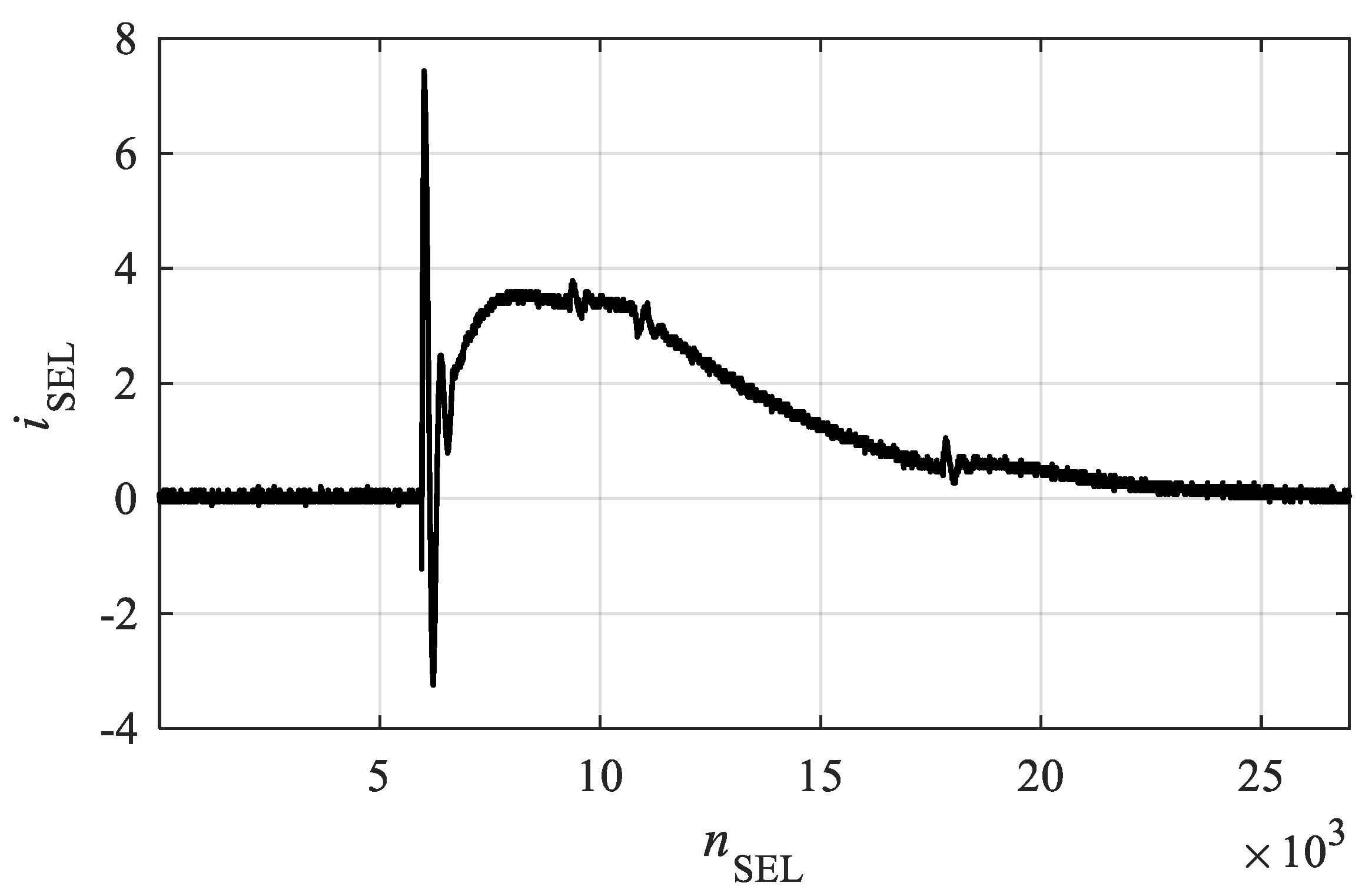
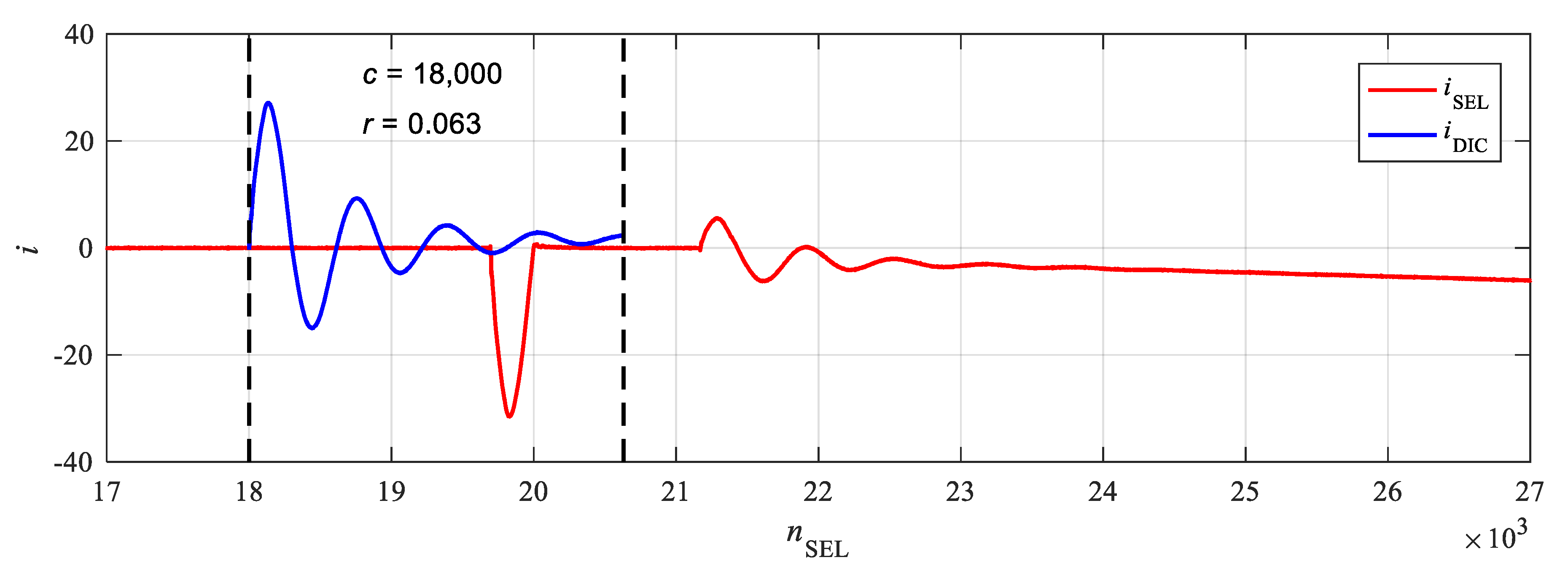
2.3. Selection of Current Samples

The result of data acquisition is the current vector $\mathit{i}=\left[i_1\dots i_N\right]$ (see Figure 5). It contains current samples recorded around (before and after) the pulse manifestation.

Due to the effectiveness of further calculations, only a selected fragment of the current vector is analyzed. This is because some fragments of the obtained current data do not contain useful information. Specifically, the current vector contains data measured prior to generating the current pulse (e.g., current vector samples from 1 to 125,000 in Figure 5). The data in this fragment of the current vector bear no information characteristic for the tested EA.

The most relevant is the fragment of the current vector near the largest pulse peak. Therefore only part of the original vector (i.e., ${\mathit{i}}_{\mathrm{SEL}}$) is extracted for analysis. The vector $\mathit{i}$ is filtered by the high-pass filter with a cut-off frequency of 1 kHz, which enables effective suppression of the 50 Hz component and its harmonics (100 Hz, 150 Hz, and so on). Then, the maximum of the high-frequency components (i.e., above 10 kHz) is found. The vector ${\mathit{i}}_{\mathrm{SEL}}$ contains 2700 selected samples around the maximum of the high-frequency components. Figure 6 shows example of the ${\mathit{i}}_{\mathrm{SEL}}$ vector.

2.4. Preparation of a Dictionary of Transients

The dictionary of transients D is a set of selected fragments of the current vectors containing pulses for various appliances:

$$D=\left\{{\mathit{i}}_{\mathrm{DIC}}^{\left(1\right)}, {\mathit{i}}_{\mathrm{DIC}}^{\left(2\right)}, \dots , {\mathit{i}}_{\mathrm{DIC}}^{\left(l_{\mathrm{D}}\right)}, \dots {\mathit{i}}_{\mathrm{DIC}}^{\left(LDIC\right)}\right\},$$

(1)

where ${\mathit{i}}_{\mathrm{DIC}}^{\left(l_{\mathrm{D}}\right)}$ are the most interesting fragments of vectors i describing the pulse and $LDIC$ is the number of examples. Figure 7 shows the method of preparing the dictionary. Samples from vector $\mathit{i}$ are selected as in Section 2.3. Then, the initial and terminal indexes of the transition are marked, leading to the structure presented below.

The marking process is performed by specifying the initial $n_{\mathrm{START}}$ and terminal $n_{\mathrm{STOP}}$ indexes. The fragment ${\mathit{i}}_{\mathrm{DIC}}$ is then extracted as follows:

$${\mathit{i}}_{\mathrm{DIC}}=\left[i_{\mathrm{DIC},1}\dots i_{\mathrm{DIC},N_{\mathrm{DIC}}}\right]=\left\{i_{\mathrm{SEL},n_{\mathrm{START}}}, i_{\mathrm{SEL},n_{\mathrm{START}}+1}, \dots , i_{\mathrm{SEL},n_{\mathrm{STOP}}-1}, i_{\mathrm{SEL},n_{\mathrm{STOP}}}\right\},$$

(2)

where $N_{\mathrm{DIC}}=n_{\mathrm{STOP}}-n_{\mathrm{START}}+1$ denotes the number of samples in ${\mathit{i}}_{\mathrm{DIC}}$.

Figure 8 shows the example of ${\mathit{i}}_{\mathrm{SEL}}$ with the marked indices $n_{\mathrm{START}}$ and $n_{\mathrm{STOP}}$ (a) and the extracted ${\mathit{i}}_{\mathrm{DIC}}$ (b).

For each considered EA, 10 examples of transition states were added to the dictionary. They differ in amplitude and shape. The selected number is the compromise between the variety of stored data and the computational effort required to obtain examples. An example is a current vector and corresponding category from the set $D_{\mathrm{CAT}}$ (which cardinality determines the number of identified appliances N_EA). Therefore, the number of vectors ${\mathit{i}}_{\mathrm{DIC}}$ in the dictionary is $LDIC=10·N_{\mathrm{EA}}$.

2.5. Determining the Cross-Correlation

In this stage, the maximum correlation between the measured signal ${\mathit{i}}_{\mathrm{SEL}}$ and subsequent dictionary entries ${\mathit{i}}_{\mathrm{DIC}}$ is found. The vector ${\mathit{i}}_{\mathrm{SEL}}$ is longer than the current vector from the dictionary ${\mathit{i}}_{\mathrm{DIC}}$, so the correlation is calculated for all possible shifts between ${\mathit{i}}_{\mathrm{DIC}}$ and ${\mathit{i}}_{\mathrm{SEL}}$.

The vector ${\mathit{i}}_{\mathrm{SEL}}$ has $N_{\mathrm{SEL}}=\mathrm{120,000}$ samples (representing the duration of 4 ms for sampling frequency $f_S=30 \mathrm{MHz}$). The correlation will be determined many times for each transition state. Therefore, the method of determining the cross-correlation should be computationally efficient. The determination of the cross-correlation without normalization was considered due to the simplicity and efficiency of calculations. In the discussed problem, the cross-correlation without normalization cannot be used, because the elements of current vectors mainly contain a fundamental component of the current signal with a frequency of 50 Hz. On the other hand, pattern vectors only contain components with frequencies at least 200 times greater than the fundamental component. The 50 Hz frequency component significantly changes the average value of the current vector, and as a result, significantly affects the value of cross-correlation without the normalization. The measure of similarity between sample vectors based on the Pearson correlation coefficient was used. The mean and standard deviation for each fragment of the vector ${\mathit{i}}_{\mathrm{SEL}}$ was calculated, which requires significant computational effort. Therefore, the optimized calculation method [36] was used.

As a result, vectors of correlations r and shifts $\mathit{c}$ were obtained. Figure 9, Figure 10 and Figure 11 illustrate the procedure.

Figure 12a shows the cross-correlation vector $\mathit{r}$ as a function of delay $\mathit{c}$ for the example of measurement data. Figure 12b shows the same relationship for the vector fragment $\mathit{r}$ with the highest correlation values.

2.6. Signature Calculation

The signature parameters are the maximum cross-correlation determined between the current vector ${\mathit{i}}_{\mathrm{SEL}}$ and all current vectors ${\mathit{i}}_{\mathrm{DIC}}^{\left(l_{\mathrm{D}}\right)}$ from the dictionary of transients. Correlation vectors for successive current vectors ${\mathit{i}}_{\mathrm{DIC}}^{\left(l_{\mathrm{D}}\right)}$ are denoted as $r_{l_{\mathrm{D}}}$. The set of categories $D_{\mathrm{CAT}}$ from the dictionary of transitions is used to name successive signature features. The idea is presented in Figure 13.

The EA signature contains maximum values of the cross-correlation between the analyzed current vector and the individual dictionary elements. Signature features are determined as the maximum absolute value of the cross-correlation ${\mathit{r}}_{l_{\mathrm{D}}}$ between the analyzed current vector ${\mathit{i}}_{\mathrm{SEL}}$ and the stored current vector ${\mathit{i}}_{\mathrm{DIC}}^{\left(l_{\mathrm{D}}\right)}$:

$$\mathrm{COR}\_x\_y=\max \left|r_{l_{\mathrm{D}}}\right|,$$

(3)

where $x\in \left\{1,\dots ,N_{\mathrm{EA}}\right\},y\in \left\{\mathrm{A},\mathrm{B},\mathrm{C},\mathrm{D},\mathrm{E},\mathrm{F},\mathrm{G},\mathrm{H},\mathrm{I},\mathrm{J}\right\}$.

The computed cross-correlation with the marked maximum value for sample measurement data are presented in Figure 14.

A signature $s_l$ consists of $P_{\mathrm{HF}-\mathrm{COR}}=10·N_{\mathrm{EA}}$ features, arranged in a specific order. Names of features and their acronyms are listed in

Table 1. Signature features in the HF-COR method.

$\mathit{p}$	Full Name	Acronym
1	The highest value of the correlation module with example A of the EA dictionary with the category number 1	COR_1_A
2	The highest value of the correlation module with example B of the EA dictionary with the category number 1	COR_ 1_B
3	The highest value of the correlation module with example C of the EA dictionary with the category number 1	COR_ 1_C
⁞	⁞	⁞
$P_{\mathrm{HF}-\mathrm{COR}}$	The highest value of the correlation module with the example J of the EA dictionary with the category number $N_{\mathrm{EA}}$	COR_NEA_J

.

$$s_l={\left[s_{l,1}\dots s_{l,p}\dots s_{l,P_{\mathrm{HF}-\mathrm{COR}}}\right]}^T.$$

(4)

Signature vectors for individual transient states constitute successive columns of the signature array $\mathit{S}$:

$$\mathit{S}=\left[{\mathit{s}}_1\dots {\mathit{s}}_l\dots {\mathit{s}}_{LSP}\right],$$

(5)

where $LSP$ is the total number of transients processed.

3. Signature Quality Assessment Method

The signature well describes devices if its features allow for distinguishing between them. Feature vectors for the same appliance should be similar to each other. The purpose of the signatures quality assessment is to verify if they can be used to identify appliances.

The process is presented in Figure 15. Division of available data into training and testing sets is important. The K-fold Cross-Validation (CV) with $K=10$ was used here. The data set is split K times into training and testing subsets (with the ratio of 9:1) in such a way that each EA is represented by the single signature in the testing set. The training sets were used to extract knowledge for the intelligent classifier, while the testing ones were applied to verify their generalization abilities. The classification accuracy was averaged on all trials.

The classifier processes signatures ${\mathit{S}}_{\mathrm{test}}^{(k)}$ to predict appliance identifiers (represented by category estimates ${\widehat{\mathit{y}}}_{\mathrm{test}}^{(k)}$). The latter are compared to actual categories ${\mathit{y}}_{\mathrm{test}}^{(k)}$ so sample errors can be calculated. Among many types of candidates for classifiers, the following were selected:

• Decision Tree (DT) representing rule-based decision systems,
• Artificial Neural Network (ANN) representing numerical decision-making systems,
• the k-Nearest Neighbors (kNN) classifier representing distance-based systems.

For each round of the CV, each classifier is trained and tested separately (see Figure 16). This way all approaches can be compared. Also, their fusion may be applied if necessary. Each algorithm has specific advantages and hyperparameters. For instance, DT during training selects features based on which rules are constructed. This is the problem for kNN, where the subset of signature values must be manually selected or weighted. Also, the number of neighbors influences diagnostic accuracy. One CV round produces four vectors:

• actual appliances identifiers in the testing set—${\mathit{y}}_{\mathrm{test}}^{(k)}$,
• category estimates based on ANN prediction—${\widehat{\mathit{y}}}_{\mathrm{NN}}^{(k)}$,
• category estimates based on DT prediction—${\widehat{\mathit{y}}}_{\mathrm{DT}}^{(k)}$,
• category estimates based on kNN prediction—${\widehat{\mathit{y}}}_{\mathrm{kNN}}^{(k)}$.

3.1. Decision Tree

The DT is a tool storing knowledge in the form of a tree (Figure 17). Nodes indicated by circles represent tests on the selected feature (in our case, one of the signature parameters) and its threshold value (like x₁ > 15). The result of the test redirects the analyzed vector of features to the node one level below until the terminal node (leaf) is reached. The leaves (rectangles) represent appliance categories. Classification of the example is then based on exploring the tree from the root (yellow node) to one of the leaves. Tests performed at each node indicate which way to take next. Generation of the DT is done using one of the machine learning algorithms like C4.5 or CART, which differ in the method of selecting tests for nodes.

3.2. Neural Network

The ANN is widely used in classification. The feed-forward structures, like multilayered perceptrons or RBF networks, are the most popular. Their hyperparameters include the number of hidden layers or the number of neurons in them $s_{\mathrm{HL}}$. Also, the output layer category coding is important, depending on the activation functions (like sigmoidal ones or softmax). The optimal structure of ANN is then found to maximize the classification accuracy for the minimum number of neurons. Knowledge extraction is performed using gradient-based algorithms.

3.3. K-Nearest Neighbors

The kNN classifier is one of the simplest non-parametric classification methods. Using the distance measure, k examples from the dictionary closest to the classified feature vector are found. The analyzed example is assigned to the categories supported by the majority of k voting vectors. The hyperparameters include the value of k, voting strategy, and the distance measure selection. This is the only one of the applied classifiers not extracting knowledge from data during the machine learning process. The problem here is determining the significance of available features, for example, by using the information capacity or correlation methods. In the presented research the DT was used to preselect them for the Euclidean measure calculation between each pair of examples $l_1$ and $l_2$:

$$d_{\mathrm{EUCLID},l_1,l_2}=\sqrt{\left(S_{l_1,p_{\mathrm{DT}}}-S_{l_2,p_{\mathrm{DT}}}\right){\left(S_{l_1,p_{\mathrm{DT}}}-S_{l_2,p_{\mathrm{DT}}}\right)}^T},$$

(6)

where $\mathit{S}$ denotes the signature array and ${\mathit{p}}_{\mathrm{DT}}$ is the number of the signature features selected by DT.

3.4. Classification Accuracy

The standard method of evaluating the classifier in the multi-category identification problem is the confusion matrix. To determine the overall quality, the accuracy should be calculated as the number of correctly identified examples from the testing set. This can be done for each category $n_{\mathrm{EA}}$ separately:

$${\eta }_{n_{\mathrm{EA}}}=\frac{\left|LS{P}_{\mathrm{EA}}:y=\widehat{y}\right|}{\left|LS{P}_{\mathrm{EA}}\right|}$$

(7)

or on the whole set (of $N_{\mathrm{EA}}$ categories):

$${\eta }_{\mathrm{ALL}}=\frac{1}{N_{\mathrm{EA}}}·\frac{\left|LS{P}_{}:y=\widehat{y}\right|}{\left|LS{P}_{}\right|}$$

(8)

4. Experimental Results

The following section discusses details of experiments, including the laboratory test stand, collected data, and classification results.

The HF-GEN method was tested in the laboratory conditions on a fixed set of 15 appliances. For each of them, 150 current pulses were recorded. From the vector $\mathit{i}$ in the transient state $l$ a signature vector ${\mathit{s}}_l$ was obtained. The signature set $\mathit{S}$ contains all $LSP$ signature vectors.

The used EAs included a vacuum cleaner, a slow juicer, an “Osram” light bulb, the “Philips” light bulb, an “Omega” light bulb, a “Lexman” lamp with four bulbs, a laptop, irons, sharpeners, grinders, kettle, jigsaw, coffee machine, air conditioner and planer.

4.1. Laboratory Test Stand

The measurement system consists of the single analyzed electrical appliance (EA), a current-voltage converter of the SCT-013-020 (CVC) type, the Advantech PCIE-1744 data acquisition card (AC), signal generator (GEN), and computer (PC) with the LabVIEW-based virtual instrument (SW) installed. The EA was connected to the power network. The CVC was installed on the L1 cable supplying EA through the resistor $R=47 \Omega$. The GEN input-output (I/O) connectors were connected to L1 and N power cables. The AC was configured in such a way that the high level of the sync voltage $u_{\mathrm{SYN}}(t)$ applied to the synchronization input would trigger the acquisition of the signal $u_{\mathrm{AD}}(t)$ fed to an analog input. The signal $u_{\mathrm{AC}}(t)$ was recorded for 10 ms since the occurrence of the high level of synchronization voltage $u_{\mathrm{SYN}}(t)$. The AC sampling rate was 30 MS/s. The data stream $i_n$ containing the samples was captured by a SW running on a PC and saved in the *.tdms file format.

The pulse signal generator consisted of AL, i.e., a lamp with an “Osram” LED bulb, (type AB30526) and a “Relpol” relay (type RM699V-3011-85-1005-RE), voltage transformer (MC-GEN), Advantech PCIE-1816H acquisition card containing an analog-to-digital converter (AD-GEN) and digital output (DO) and a computer (PC-GEN) running the virtual instrument (CS). AL was connected to the supply network via the RE relay, while MC-GEN—to the supply network via the L1 and N conductors. The CVC of the type SCT-013-020 type converts voltage $u(t)$ to $u_{\mathrm{AD}-\mathrm{GEN}}(t)$. Its measuring range is about 120A. Laboratory tests proved that SCT-013-020 allows for accurate measurements of signals with frequency up to 400 kHz which is enough for the presented HF-GEN method. The voltage $u_{\mathrm{AD}-\mathrm{GEN}}(t)$ was fed to the analog input no 0 (AD-GEN) of the acquisition card.

AD-GEN samples voltage $u_{\mathrm{AD}-\mathrm{GEN}}(t)$ at 250 kS/s. Based on them, CS detects the voltage phase by actuating a logic signal $o_n$. The AL is switched on when the voltage $u(t)$ reaches the value of $300 \mathrm{V}$. DO converts logic signal $o_n$ to voltage $u_{\mathrm{SYN}}(t)$. The RE becomes closed when the high state appears on $u_{\mathrm{SYN}}(t)$.

4.2. Measurement Procedure

During experiments, the following measurement procedure was implemented:

• Connecting to the power grid and switching on EA under test;
• Setting CS so that the GEN generates a pulse signal 150 times (in the case of its acquisition for quality evaluation) or at least 10 times (for the transients’ dictionary);
• Setting the SW to acquire all current pulses;
• Starting the impulse generation and acquisition process;
• Switching off the tested device.

These steps are performed for each tested EA. A separate series of measurements is carried out with no EA connected (only steps 2–4 are then taken).

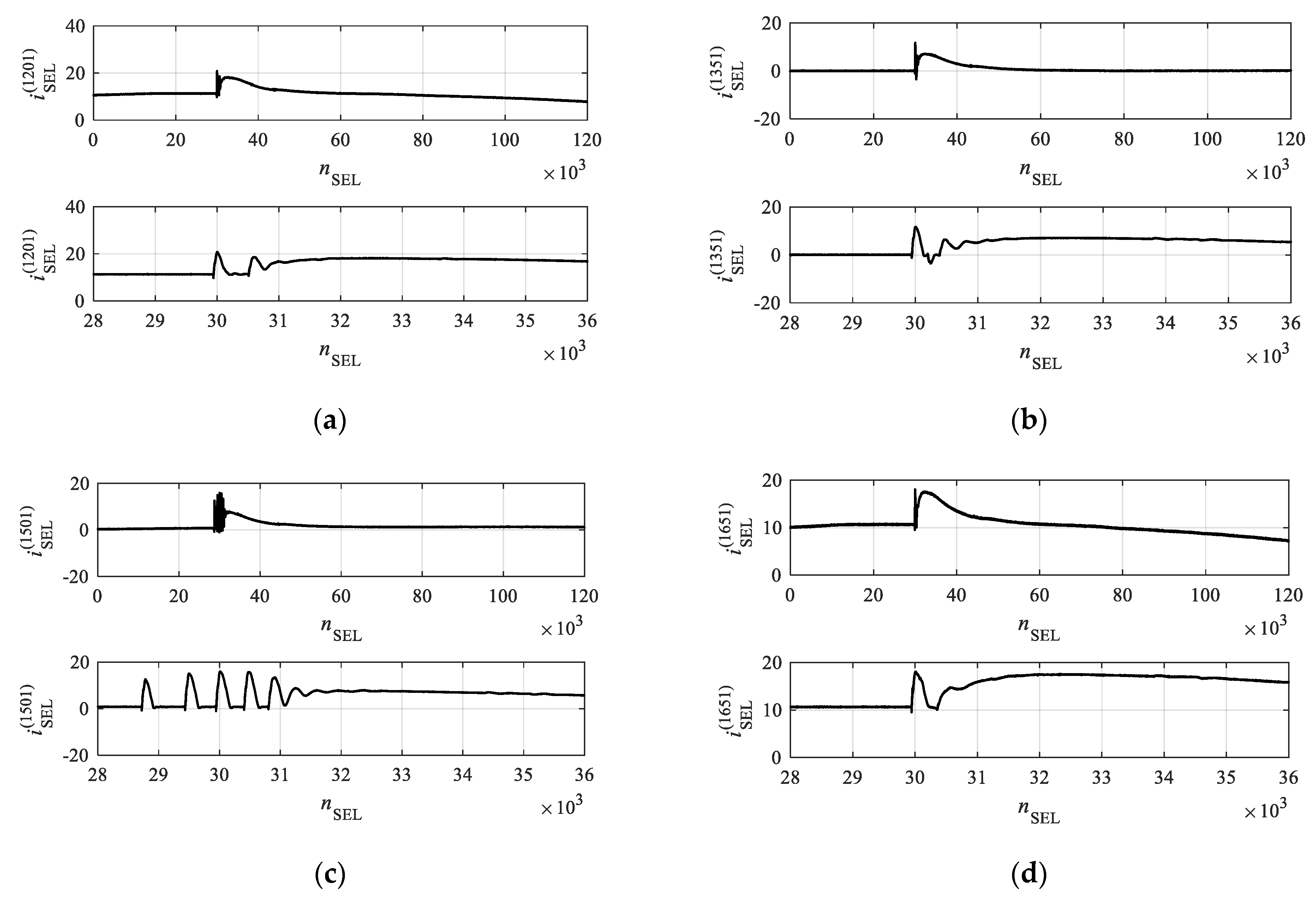
4.3. Analysis of Measured Current Vectors

As a result of measurements for 16 categories (15 types of EA and no-EA), $150\times 16=2400$ vectors of current samples were collected. Details of the recorded vectors are in

Table 2. Information on recorded current vectors.

$\mathbf{Category}\mathbf{Number}{\mathit{n}}_{\mathbf{EA}}$	EA Name	Type	Nominal Power	$\mathbf{Indexes}\mathbf{of}\mathbf{Current}\mathbf{Vectors}\mathit{l}$
0	no EA	-	-	1…150
1	vacuum cleaner	Zelmer ZVC425HT	1000 W	151…300
2	slow juicer	Eldom PJ400	400 W	301…450
3	lamp with LED bulb “Osram”	Osram AB42758	11.5 W	451…600
4	lamp with LED bulb “Philips”	Philips 9290012345C	13 W	601…750
5	lamp with LED bulb “Omega”	no data	11 W	751…900
6	wall lamp with four LED bulbs “Lexman”	no data	5 W	901…1050
7	laptop	Dell PP36L	100–240 V ~1.6 A	1051…1200
8	iron	Philips GC 4410	2000–2400 W	1201…1350
9	sharpener	SilverCrest SEAS 20 B1	20 W	1351…1500
10	grinder	Makita GB801	550 W	1501…1650
11	kettle	Zelmer CK1004	1850–2200 W	1651…1800
12	jigsaw	Bosch GST 90 BE	650 W	1801…1950
13	coffee machine	Saeco HD8917	1850 W	1951…2100
14	air conditioner	Cooper&Hunter CH-S09RX4	2700–2850 W	2101…2250
15	planer	Makita 2012NB	1650 W	2251…2400

. Each current vector $\mathit{i}$ has 300,000 samples (representing duration of 10 ms).

The current vectors were selected according to Section 2.3. The result were current vectors ${\mathit{i}}_{\mathrm{SEL}}$ which length of $N_{\mathrm{SEL}}=\mathrm{120,000}$ (duration of 4 ms). The vectors ${\mathit{i}}_{\mathrm{SEL}}^{(l)}$ for selected examples $l$ are in Figure 18 and Figure 19.

The average current value ${\mathit{i}}_{\mathrm{SEL}}^{(l)}$ depends on the analyzed EA. For instance, examples $l\in \{151,1201,1651,2251\}$ representing vacuum cleaner, iron, kettle, and planer are characterized by relatively high power. The pulses are generated for the voltage $u=300 \mathrm{V}$ when the instantaneous current levels of EAs are close to the maximum value. Therefore, a high average current value is observed here.

The direction of the pulse current is always the same. It results from forcing the voltage phase at the moment of generating the pulse.

All waveforms presented in Figure 18 and Figure 19 are characterized by a rise in the average current value starting approx. at $n_{\mathrm{SEL}}=\mathrm{30,000}$. In turn, for the $n_{\mathrm{SEL}}=\mathrm{34,000}\dots \mathrm{50,000}$ current values drop until reaching the level as before the pulse appearance.

For examples $l\in \{1,1201,1501\}$, the multiple contact of the RE is visible in the form of many similar oscillations which quickly converge to the average current value ${\mathit{i}}_{\mathrm{SEL}}^{(l)}$. For category 0 (no EA), this oscillation is visible for the $n_{\mathrm{SEL}}=\mathrm{29,400}$, while for category 8 (iron) it is for $n_{\mathrm{SEL}}=\mathrm{30,000}$, and for category 10 (grinder), 4 such oscillations are visible for $n_{\mathrm{SEL}}\in \left\{\mathrm{28,800},\mathrm{29,500},\mathrm{30,000},\mathrm{30,500}\right\}$.

The starting point for further analysis is the current vector obtained for category 0 when no EA is connected. The shape of the pulse for the example $l=1$ (Figure 18a) is the impulse response of AL after switching on the supply voltage. All other current vectors are the impulse response of the system in which two electricity receivers are simultaneously connected to the power supply: AL and the tested EA. The change in the shape of the current waveform ${\mathit{i}}_{\mathrm{SEL}}^{(l)}$ is proportional to the influence of the tested EA on the total impedance of these two parallelly connected loads in the supply network.

Examples $l\in \{751,901,1051\}$, i.e., lamp with bulb “Omega”, wall lamp with four bulbs ”Lexman” and kettle are similar to the example $l=1$. Examples $l=451$ (lamp with bulb ”Osram”) and $l=601$ (lamp with bulb ”Philips”) are distinguished by the lack of the minimum of the 2A-amplitude instantaneous current for $n_{\mathrm{SEL}}=\mathrm{30,300}$.

The example $l=1951$ recorded for the coffee machine has a characteristic shape, especially in the area $n_{\mathrm{SEL}}=\mathrm{30,000}\dots \mathrm{31,000}$, where rapid changes in the instantaneous current values are visible, and the characteristic for many other examples of quasi-periodic oscillations cannot be found.

A vacuum cleaner $\left(l=151\right)$, slow juicer $\left(l=301\right)$, jigsaw $\left(l=1801\right)$, and planer $\left(l=2251\right)$ reduce the frequency of current oscillations, and increase the number of visible oscillations, which is unique for each EA. Specifically, for example $l=151$, five oscillations have period of approximately 940 samples corresponding to a frequency of 31.9 kHz. For the example $l=301$(slow juicer), four periods exist (923 samples each) which corresponds to a frequency of 32.5 kHz. For the example $l=1801$ (jigsaw), five periods of 500 samples correspond to a frequency of 60 kHz. For the example $l=2251$ (planer), there are six periods, each 610 samples long, which corresponds to a frequency of 49.2 kHz. All these categories have motors, which may shape the current pulse.

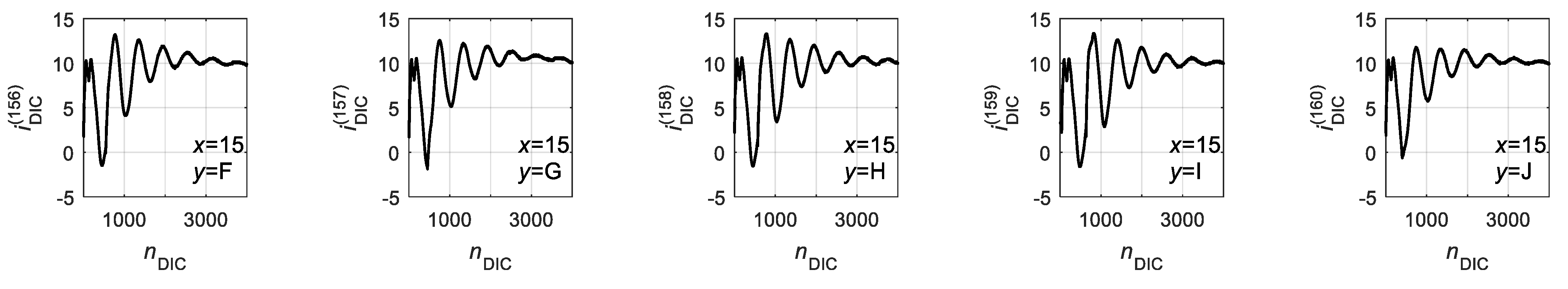
4.4. Dictionary of Transients

The measurement data for the transient dictionary does not coincide with the measurement data used to train and test the classification algorithms. The set of measurement data used in the transient state dictionary was prepared independently of the data set described in Section 4.3. Selection of current vectors for the dictionary does not disturb the obtained classification results.

To prepare the dictionary of transients, the procedure presented in Section 2.4 was used. For each of sixteen categories, 10 examples of transient current $\mathit{i}$ were collected, from which current vectors ${\mathit{i}}_{\mathrm{SEL}}$ were obtained. The resulting dictionary of transients is presented in

Table 3. Information about the transient dictionary.

Category Number $\mathit{x}$	Device Name	$\mathbf{Indexes}\mathbf{of}\mathbf{Current}\mathbf{Vectors}{\mathit{l}}_{\mathbf{D}}$	Signature Features Related to the Dictionary Examples
0	no EA	1…10	COR_0_A…COR_0_J
1	vacuum cleaner	11…20	COR_1_A…COR_1_J
2	slow juicer	21…30	COR_2_A…COR_2_J
3	lamp with bulb “Osram”	31…40	COR_3_A…COR_3_J
4	lamp with bulb “Philips”	41…50	COR_4_A…COR_4_J
5	lamp with bulb “Omega”	51…60	COR_5_A…COR_5_J
6	wall lamp with five “Lexman” bulbs	61…70	COR_6_A…COR_6_J
7	Laptop	71…80	COR_7_A…COR_7_J
8	Iron	81…90	COR_8_A…COR_8_J
9	Sharpener	91…100	COR_9_A…COR_9_J
10	Grinder	101…110	COR_10_A…COR_10_J
11	Kettle	111…120	COR_11_A…COR_11_J
12	Jigsaw	121…130	COR_12_A…COR_12_J
13	coffee machine	131…140	COR_13_A…COR_13_J
14	air conditioner	141…150	COR_14_A…COR_14_J
15	Planer	151…160	COR_15_A…COR_15_J

. The most important fragments of current vectors ${\mathit{i}}_{\mathrm{DIC}}^{\left(l_{\mathrm{D}}\right)}$ for selected categories are in Figure 20, Figure 21, Figure 22 and Figure 23.

Despite ensuring similar conditions for generating impulses, the current vectors ${\mathit{i}}_{\mathrm{DIC}}$ for the no-EA category (Figure 20) differ from each other. The first difference between examples is the multiple contact phenomenon described in Section 4.3, visible for the examples $l_{\mathrm{D}}\in \left\{5,6,10\right\}$.

In all waveforms, a quasi-periodic oscillation is present, disappearing after about three periods. A characteristic of these vectors is a rising edge on which the oscillation is located. In the example $l_{\mathrm{D}}=7$, the slope is visible for $n_{\mathrm{DIC}}=1\dots 2000$. The rising edge is a characteristic feature of applied AL.

For dictionary examples representing the vacuum cleaner (Figure 21), three types of waveforms can be distinguished. They differ mainly in the shape of the initial part of the vector ${\mathit{i}}_{\mathrm{DIC}}$ ($n_{\mathrm{DIC}}=1\dots 1000$). The first type is present in examples $l_{\mathrm{D}}=11$ and $l_{\mathrm{D}}=19$. The second type is visible in examples $l_{\mathrm{D}}\in \{14,15,18\}$, while the third one—in examples $l_{\mathrm{D}}\in \{12,13,16,17,20\}$. The oscillation frequency in the second part of the vector ${\mathit{i}}_{\mathrm{DIC}}$ is lower than in the no EA case (category 0 in Figure 20). Duration of the oscillation between samples $n_{\mathrm{DIC}}=1000$ and $n_{\mathrm{DIC}}=4000$ is the same for all vectors in this category with period of about 940 samples, which corresponds to a frequency of 31.9 kHz.

Waveforms in Figure 22 represent lamps with the “Osram” bulb. Here, the multiple-contact phenomenon of the relay is visible, especially for the example $l_{\mathrm{D}}=40$, where four similar oscillations are present in the first part of the current vector.

Vectors for the planer (Figure 23) are different from other appliances, and at the same time, they are similar to each other. Their distinguishing feature is the shape of the first part of the vector ${\mathit{i}}_{\mathrm{DIC}}\left(n_{\mathrm{DIC}}=1\dots 300\right)$. Here examples $l_{\mathrm{D}}\in \{151,153,154,155\}$ have one maximum above the slope of the oscillation. It is present around the sample $n_{\mathrm{DIC}}=100$. Examples $l_{\mathrm{D}}\in \{152,156,157,158,159,160\}$ have two visible maxima, one for $n_{\mathrm{DIC}}=90$ and the other one at $n_{\mathrm{DIC}}=190$. In all examples for the planer, at least five periods of oscillation with a period of about 610 samples are present, corresponding to a frequency of about 49.2 kHz.

4.5. Signature Parameters

Based on the determined correlation vectors for each pair of the transition (for $l=1\dots 2400$) and the dictionary example $l_{\mathrm{D}}=1\dots 160$, the values of features in the signature $\mathit{S}$ were determined. For each example $l$, the signature contains 160 features. Values of two characteristic features for each category are presented in Figure 24 and Figure 25.

The COR_1_A feature (Figure 24) can be used to distinguish between three categories: 1 (vacuum cleaner), 2 (slow juicer), and 13 (coffee machine). A majority of examples belonging to these categories have the value of the COR_1_A in the range between 0.97 and 1.0. Almost all observations of the remaining categories assume values of this feature in the range 0.85–0.97, so it is not suitable for distinguishing between them.

The COR_9_F (Figure 25) feature is characterized by high values for almost all examples. Only three vectors from category 3 (lamp with the “Osram” bulb) have COR_9_F values below 0.85. Observations for all other categories assume values of this feature in the range 0.85–1. Even though the COR_9_F feature was determined for the dictionary examples belonging to the grinder category, the value distribution of this feature is similar for each category. Therefore it is not useful in most cases.

4.6. Classification Results

This section presents results of three classifiers’ operation for the available data partitioned using the K-fold cross validation (where K = 10).

4.6.1. Neural Network

The application of ANN required selecting the optimal number of neurons in the hidden layer. For that purpose, the network was trained many times, with the number of neurons in the hidden layer ranging from 1 to 24. The classification error as a function of the number of neurons in the hidden layer is in Figure 26.

The total classification error is minimal for 15 neurons in the hidden layer. Further increase of this parameter does not significantly affect the classification error.

The confusion matrix ${\mathit{C}}_{\mathrm{NN}}$ and the classification accuracy ${\eta }_{n_{\mathrm{EA}}, \mathrm{NN}}$ for 16 examined categories in the optimal ANN structure are presented in

Table 4. Confusion matrix and the classification accuracy of the neural network for 15 neurons in the hidden layer.

		Assigned Category																${\mathit{\eta }}_{{\mathit{n}}_{\mathbf{EA}}, \mathbf{NN}}$
		0	1	2	3	4	5	6	7	8	9	10	11	12	13	14	15
True Category	0	89	0	0	14	0	0	15	0	2	20	9	0	0	0	1	0	59%
	1	0	147	3	0	0	0	0	0	0	0	0	0	0	0	0	0	98%
	2	0	3	146	0	0	0	0	0	0	0	0	0	0	0	0	1	97%
	3	40	0	0	42	0	0	6	1	0	30	31	0	0	0	0	0	28%
	4	0	0	0	0	73	76	0	0	1	0	0	0	0	0	0	0	49%
	5	0	0	0	0	32	117	0	0	0	0	0	1	0	0	0	0	78%
	6	31	0	0	8	0	1	106	0	0	3	1	0	0	0	0	0	71%
	7	0	0	0	0	0	1	0	148	1	0	0	0	0	0	0	0	99%
	8	0	0	0	0	4	2	0	0	142	1	1	0	0	0	0	0	95%
	9	21	0	0	30	0	0	5	1	1	36	56	0	0	0	0	0	24%
	10	11	0	0	13	0	0	2	0	0	31	93	0	0	0	0	0	62%
	11	0	0	0	0	0	1	0	0	0	0	0	149	0	0	0	0	99%
	12	0	0	0	0	0	0	0	0	0	0	0	0	150	0	0	0	100%
	13	0	0	0	0	0	0	0	0	0	0	0	0	0	150	0	0	100%
	14	0	0	0	0	0	0	0	0	0	0	0	0	0	0	150	0	100%
	15	0	0	0	0	0	0	0	0	0	0	0	0	1	0	0	149	99%

.

The overall classification accuracy was as follows:

$${\eta }_{\mathrm{ALL},\mathrm{NN}}=\frac{1}{16}{\displaystyle \sum _{n_{\mathrm{EA}}=0}^{15}{\eta }_{n_{\mathrm{EA}},\mathrm{NN}}}=78.6\%.$$

(9)

The accuracy of at least 95% was obtained for nine appliances: 1 (vacuum cleaner), 2 (slow juicer), 7 (laptop), 8 (iron), 11 (kettle), 12 (jigsaw), 13 (coffee machine), 14 (air conditioner), and 15 (planer). Signatures for EAs 11–15 significantly differ from all others, which makes them easily identifiable (see columns 11–15). The lowest classification accuracy (24%) was achieved for category 9 (sharpener) and for category 3 (lamp with the “Osram” bulb) at the level of 28%. Total 56 (37%) examples of category 9 were incorrectly assigned to category 10. More than a half (51%) of examples of category 4 (lamp with the “Philips” bulb) were incorrectly assigned to category 5 (lamp with the “Omega” bulb). This is because categories 4 and 5 have similar signatures.

4.6.2. Decision Tree

None of the categories was faultlessly identified by DT (see

Table 5. Confusion matrix and classification accuracy for the decision tree algorithm.

		Assigned Category																${\mathit{\eta }}_{{\mathit{n}}_{\mathbf{EA}}, \mathbf{DT}}$
		0	1	2	3	4	5	6	7	8	9	10	11	12	13	14	15
True Category	0	60	0	0	25	3	1	28	1	3	25	4	0	0	0	0	0	40%
	1	0	143	3	0	0	0	0	0	0	0	0	0	0	4	0	0	95%
	2	0	5	140	0	0	0	0	3	0	0	0	1	0	1	0	0	93%
	3	29	0	0	44	0	0	14	1	0	36	26	0	0	0	0	0	29%
	4	0	0	0	0	111	33	2	2	1	0	0	0	0	0	1	0	74%
	5	1	0	0	0	39	105	2	0	1	0	0	0	0	0	2	0	70%
	6	23	0	0	11	2	1	100	2	0	9	2	0	0	0	0	0	67%
	7	2	0	2	0	0	0	1	136	3	2	3	0	0	1	0	0	91%
	8	2	0	2	1	4	1	0	0	134	1	0	3	0	0	2	0	89%
	9	25	0	0	33	1	1	7	2	2	57	22	0	0	0	0	0	38%
	10	8	0	0	30	0	0	6	0	0	28	78	0	0	0	0	0	52%
	11	0	0	2	0	0	0	0	3	5	0	0	139	1	0	0	0	93%
	12	0	0	0	0	0	1	0	0	1	0	0	0	145	0	2	1	97%
	13	0	3	0	0	0	0	0	1	0	0	0	0	0	146	0	0	97%
	14	1	0	0	0	0	0	0	0	3	1	0	0	0	0	145	0	97%
	15	0	0	0	0	1	2	0	0	0	0	0	1	0	0	0	146	97%

). The best score of 97% was obtained for appliances 12 (jigsaw), 13 (coffee machine), 14 (air conditioner), and 15 (planer). For category 1 (vacuum cleaner), the accuracy was 95%. Categories 12 and 15 have very few examples from other incorrectly assigned categories. The worst classification result (29%) was obtained for category 3 (lamp with “Osram” bulb). There are also two groups of indistinguishable appliances. The first one consists of categories 0 (no EA), 3 (lamp with the “Osram” bulb), 6 (wall lamp with four “Lexman” bulbs), 9 (sharpener), and 10 (grinder). The second group consists of category 4 (lamp with bulb “Philips”) and 5 (lamp with bulb “Omega”). The overall classification efficiency was as follows:

$${\eta }_{\mathrm{ALL},\mathrm{DT}}=\frac{1}{16}{\displaystyle \sum _{n_{\mathrm{EA}}=0}^{15}{\eta }_{n_{\mathrm{EA}},\mathrm{DT}}}=76.2\%.$$

(10)

4.6.3. The kNN Algorithm

To identify the most significant predictors, the DT was first trained for all 2400 examples of transients. In the DT training process, 82 signature features were selected as the most significant ones. Using selected features, a classification was made for each of the 10 cross-validation attempts. The confusion matrix $C_{\mathrm{kNN}}$ for all cross-validation trials and the classification accuracy ${\eta }_{n_{\mathrm{EA}}, \mathrm{kNN}}$ is presented in

Table 6. Confusion matrix and classification accuracy for the k-nearest neighbors algorithm.

		Assigned Category																${\mathit{\eta }}_{{\mathit{n}}_{\mathbf{EA}}, \mathbf{kNN}}$
		0	1	2	3	4	5	6	7	8	9	10	11	12	13	14	15
True Category	0	70	0	0	38	0	1	14	2	1	17	7	0	0	0	0	0	47%
	1	0	149	1	0	0	0	0	0	0	0	0	0	0	0	0	0	99%
	2	0	3	147	0	0	0	0	0	0	0	0	0	0	0	0	0	98%
	3	38	0	0	65	0	0	3	0	1	21	22	0	0	0	0	0	43%
	4	1	0	0	0	120	29	0	0	0	0	0	0	0	0	0	0	80%
	5	3	0	0	0	31	113	2	0	0	0	0	0	0	0	1	0	75%
	6	19	0	0	11	1	0	107	1	0	7	4	0	0	0	0	0	71%
	7	1	0	0	1	0	0	0	145	1	2	0	0	0	0	0	0	97%
	8	0	0	0	1	0	2	0	0	145	1	0	0	0	0	1	0	97%
	9	25	0	0	26	0	0	6	0	3	59	31	0	0	0	0	0	39%
	10	10	0	0	29	0	0	1	0	0	25	85	0	0	0	0	0	57%
	11	0	0	0	0	0	1	0	0	0	0	0	149	0	0	0	0	99%
	12	0	0	0	0	0	0	0	0	0	0	0	0	150	0	0	0	100%
	13	0	0	0	0	0	0	0	0	0	0	0	0	0	150	0	0	100%
	14	0	0	0	0	0	0	0	0	0	0	0	0	0	0	150	0	100%
	15	0	0	0	0	0	0	0	0	0	0	0	0	0	0	0	150	100%

.

The k-nearest neighbors algorithm classified nine categories with an accuracy of at least 95%. These are: 1 (vacuum cleaner), 2 (slow juicer), 7 (laptop), 8 (iron), 11 (grinder), 12 (jigsaw), 13 (coffee machine), 14 (air conditioner), and 15 (planer). Categories 11, 12, 13, and 15 have been identified flawlessly. The worst classification result (39%) was obtained for category 10 (grinder). There are two groups of similar categories: (0, 3, 6, 9, 10) and (4, 5). The overall classification efficiency is as follows:

$${\eta }_{\mathrm{ALL},\mathrm{kNN}}=\frac{1}{16}{\displaystyle \sum _{n_{\mathrm{EA}}=0}^{15}{\eta }_{n_{\mathrm{EA}},\mathrm{kNN}}}=81.4\%.$$

(11)

5. Summary

The paper presented the system for NILM task based on the transient features of the generated pulse analysis. It exploits mutual influence between devices operating in the same power circuit to identify the moment of introducing the new one.

The pulse signal generator was designed. Its task is to generate current pulses at predetermined time intervals in a fixed phase of the supply voltage. The measurement system acquires current pulses and stores them as sample vectors. A method for processing current signals was designed to determine their characteristic features based on the cross-correlation calculated for each pair of EAs. The method uses information about the phase and amplitude of all (periodic and non-periodic) components of the current pulse appearing in the transient state of the device turned on. The processing result is a signature with features characterizing the EA. The signature quality was verified using three different classifiers.

The presented experiments show that devices connected to one circuit of the supply network influence each other. A significant impact of a background device in the steady state on the current pulse on another device being turned on was observed. When a known load is switched on under repeated conditions, the change in the shape of this pulse may be characteristic for a device operating in the background. Results of the classification show that in the best case, 9 out of 15 EAs are recognizable with an accuracy of at least 97%. Satisfying results were obtained for majority of tested EAs. There are types of EA for which this method fails. Therefore multiple different identification methods should be implemented simultaneously.

In practical application of NILM system the changing set of devices operating at the same time must be considered. This makes the task difficult, as the change of the pulse shape will be a certain superposition of all working EA. Therefore additional research are required to approach this challenge. Results of presented experiments show that in the highly controlled environment (especially when only a single appliance is operating) the proposed approach provides high identification accuracy Its applicability should be further investigated in the future.

References

1. Hart, G.W. Nonintrusive Appliance Load Monitoring. Proc. IEEE 1992, 80, 1870–1891. [Google Scholar] [CrossRef]
2. Tang, G.; Wu, K.; Lei, J. A Distributed and Scalable Approach to Semi-Intrusive Load Monitoring. IEEE Trans. Parallel Distrib. Syst. 2016, 27, 1553–1565. [Google Scholar] [CrossRef]
3. Agyeman, K.A.; Han, S.; Han, S. Real-time recognition non-intrusive electrical appliance monitoring algorithm for a residential building energy management system. Energies 2015, 8, 9029–9048. [Google Scholar] [CrossRef]
4. Carrie Armel, K.; Gupta, A.; Shrimali, G.; Albert, A. Is disaggregation the holy grail of energy efficiency? The case of electricity. Energy Policy 2013, 52, 213–234. [Google Scholar] [CrossRef] [Green Version]
5. Nguyen, T.K.; Azarkh, I.; Nicolle, B.; Jacquemod, G.; Dekneuvel, E. Applying NIALM technology to predictive maintenance for industrial machines. In Proceedings of the IEEE International Conference on Industrial Technology, Lyon, France, 20–22 February 2018; pp. 341–345. [Google Scholar]
6. He, D.; Lin, W.; Liu, N.; Harley, R.G.; Habetler, T.G. Incorporating non-intrusive load monitoring into building level demand response. IEEE Trans. Smart Grid 2013, 4, 1870–1877. [Google Scholar]
7. Zeifman, M.; Roth, K. Nonintrusive appliance load monitoring: Review and outlook. IEEE Trans. Consum. Electron. 2011, 57, 76–84. [Google Scholar] [CrossRef]
8. Esa, N.F.; Abdullah, M.P.; Hassan, M.Y. A review disaggregation method in Non-intrusive Appliance Load Monitoring. Renew. Sustain. Energy Rev. 2016, 66, 163–173. [Google Scholar] [CrossRef]
9. Liszewski, K.; Łukaszewski, R.; Kowalik, R.; Łukasz, N.; Winiecki, W. Different appliance identification methods in Non-Intrusive Appliance Load Monitoring. In Advanced Data Acquisition and Intelligent Data Processing; Haasz, V., Madani, K., Eds.; River Publishers: Aalborg, Denmark, 2014; pp. 31–58. [Google Scholar]
10. Wong, Y.F.; Ahmet Sekercioglu, Y.; Drummond, T.; Wong, V.S. Recent approaches to non-intrusive load monitoring techniques in residential settings. In Proceedings of the IEEE Symposium on Computational Intelligence Applications in Smart Grid (CIASG), Singapore, 16–19 April 2013; pp. 73–79. [Google Scholar]
11. Abubakar, I.; Khalis, S.N.; Mustafa, M.W.; Shareef, H.; Mustapha, M. An Overview of Non-Intrusive Load Monitoring Methodologies. In Proceedings of the IEEE Conference on Energy Conversion (CENCON), Johor Bahru, Malaysia, 9–20 October 2015; pp. 54–59. [Google Scholar]
12. Gao, J.; Giri, S.; Kara, E.C.; Bergés, M. PLAID: A public dataset of high-resolution electrical appliance measurements for load identification research. In Proceedings of the BuildSys 2014—Proceedings of the 1st ACM Conference on Embedded Systems for Energy-Efficient Buildings, Memphis, Tennessee, 4–6 November 2014; Association for Computing Machinery: New York, NY, USA, 2014; pp. 198–199. [Google Scholar]
13. Kelly, J.; Knottenbelt, W. The UK-DALE dataset, domestic appliance-level electricity demand and whole-house demand from five UK homes. Sci. Data 2015, 2, 1–14. [Google Scholar] [CrossRef] [Green Version]
14. Renaux, D.P.B.; Pottker, F.; Ancelmo, H.C.; Lazzaretti, A.E.; Lima, C.R.E.; Linhares, R.R.; Oroski, E.; da Silva Nolasco, L.; Lima, L.T.; Mulinari, B.M.; et al. A dataset for non-intrusive load monitoring: Design and implementation. Energies 2020, 13, 5371. [Google Scholar] [CrossRef]
15. Pereira, L.; Nunes, N. Performance evaluation in non-intrusive load monitoring: Datasets, metrics, and tools—A review. Wiley Interdiscip. Rev. Data Min. Knowl. Discov. 2018, 8, 1–17. [Google Scholar] [CrossRef] [Green Version]
16. Wójcik, A.; Łukaszewski, R.; Kowalik, R.; Winiecki, W. Nonintrusive appliance load monitoring: An overview, laboratory test results and research directions. Sensors 2019, 19, 3621. [Google Scholar] [CrossRef] [PubMed] [Green Version]
17. Mauch, L.; Yang, B. A new approach for supervised power disaggregation by using a deep recurrent LSTM network. In Proceedings of the 2015 IEEE Global Conference on Signal and Information Processing, Orlando, FL, USA, 14–16 December 2016; pp. 63–67. [Google Scholar]
18. Koziy, K.; Gou, B.; Aslakson, J. A low-cost power-quality meter with series arc-fault detection capability for smart grid. IEEE Trans. Power Deliv. 2013, 28, 1584–1591. [Google Scholar] [CrossRef]
19. Wang, Z.; Zheng, G. Residential appliances identification and monitoring by a nonintrusive method. IEEE Trans. Smart Grid 2012, 3, 80–92. [Google Scholar] [CrossRef]
20. Zhao, B.; Stankovic, L.; Stankovic, V. On a Training-Less Solution for Non-Intrusive Appliance Load Monitoring Using Graph Signal Processing. IEEE Access 2016, 4, 1784–1799. [Google Scholar] [CrossRef] [Green Version]
21. Li, D.; Dick, S. Whole-house Non-Intrusive Appliance Load Monitoring via multi-label classification. In Proceedings of the International Joint Conference on Neural Networks, Vancouver, BC, Canada, 24–29 July 2016; pp. 2749–2755. [Google Scholar]
22. Henao, N.; Agbossou, K.; Kelouwani, S.; Dube, Y.; Fournier, M. Approach in Nonintrusive Type I Load Monitoring Using Subtractive Clustering. IEEE Trans. Smart Grid 2017, 8, 812–821. [Google Scholar] [CrossRef]
23. Liu, B.; Luan, W.; Yu, Y. Dynamic time warping based non-intrusive load transient identification. Appl. Energy 2017, 195, 634–645. [Google Scholar] [CrossRef]
24. Kong, W.; Dong, Z.; Xu, Y.; Hill, D. An Enhanced Bootstrap Filtering Method for Non- Intrusive Load Monitoring. In Proceedings of the 2016 IEEE Power and Energy Society General Meeting (PESGM), Boston, MA, USA, 17–21 July 2016; pp. 1–5. [Google Scholar]
25. Ducange, P.; Marcelloni, F.; Antonelli, M. A novel approach based on finite-state machines with fuzzy transitions for nonintrusive home appliance monitoring. IEEE Trans. Ind. Inform. 2014, 10, 1185–1197. [Google Scholar] [CrossRef]
26. Sultanem, F. Using appliance signatures for monitoring residential loads at meter panel level. IEEE Trans. Power Deliv. 1991, 6, 1380–1385. [Google Scholar] [CrossRef]
27. Reinhardt, A.; Burkhardt, D.; Zaheer, M.; Steinmetz, R. Electric appliance classification based on distributed high resolution current sensing. In Proceedings of the 37th Annual IEEE Conference on Local Computer Networks Workshops, Clearwater, FL, USA, 22–25 October 2012; pp. 999–1005. [Google Scholar]
28. Yoshimoto, K.; Nakano, Y.; Amano, Y.; Kermanshahi, B. Non-intrusive appliances load monitoring system using neural networks. In Proceedings of the Proceedings ACEEE Summer Study on Energy Efficiency in Buildings; 2000; Volume 7, pp. 2–5. Available online: https://www.eceee.org/static/media/uploads/site-2/library/conference_proceedings/ACEEE_buildings/2000/Panel_7/p6_17/paper.pdf (accessed on 28 January 2021).
29. Srinivasan, D.; Ng, W.S.; Liew, A.C. Neural-network-based signature recognition for harmonic source identification. IEEE Trans. Power Deliv. 2006, 21, 398–405. [Google Scholar] [CrossRef]
30. Gupta, S.; Reynolds, M.S.; Patel, S.N. ElectriSense: Single-point sensing using EMI for electrical event detection and classification in the home. In Proceedings of the 12th ACM International Conference on Ubiquitous Computing, Copenhagen, Denmark, 26–29 September 2010; pp. 139–148. [Google Scholar]
31. Torquato, R.; Acharya, J.R.; Xu, W. A Method to Determine Stray Voltage Sources—Part II: Verifications and Applications. IEEE Trans. Power Deliv. 2015, 30, 720–727. [Google Scholar] [CrossRef]
32. Duarte, C.; Delmar, P.; Goossen, K.W.; Barner, K.; Gomez-Luna, E. Non-intrusive load monitoring based on switching voltage transients and wavelet transforms. In Proceedings of the 2012 Future of Instrumentation International Workshop, Gatlinburg, TN, USA, 8–9 October 2012; pp. 101–104. [Google Scholar]
33. Duarte, C. Non-Intrusive Monitoring of Electrical Loads Based on Switching Transient Voltage Analysis: Signal Acquisition and Features Extraction; Univeristy of Delaware: Newark, DE, USA, 2013. [Google Scholar]
34. Chang, H.H.; Lian, K.L.; Su, Y.C.; Lee, W.J. Power-spectrum-based wavelet transform for nonintrusive demand monitoring and load identification. IEEE Trans. Ind. Appl. 2014, 50, 2081–2089. [Google Scholar] [CrossRef]
35. Wójcik, A.; Winiecki, W.; Łukaszewski, R.; Bilski, P. Analysis of Transient State Signatures in Electrical Household Appliances. In Proceedings of the 10th IEEE International Conference on Intelligent Data Acquisition and Advanced Computing Systems: Technology and Applications (IDAACS), Metz, France, 18–21 September 2019; pp. 639–644. [Google Scholar]
36. Lewis, J.P. Fast Normalized Cross-Correlation. Vis. Interface 2010, 120–123. [Google Scholar]
Figure 1. Illustration of the HF-GEN method.
Energies 14 00673 g001
Figure 2. Block diagram of the HF-GEN method.
Energies 14 00673 g002
Figure 3. Block diagram of the pulse signal generator.
Energies 14 00673 g003
Figure 4. Diagram of the measuring system of the HF-GEN method.
Energies 14 00673 g004
Figure 5. The sampled current vector i.
Energies 14 00673 g005
Figure 6. Current vector i SEL for sample measurement data.
Energies 14 00673 g006
Figure 7. Preparation of dictionary of transients.
Energies 14 00673 g007
Figure 8. Current vectors for the sample measurement data: i SEL (a) and i DIC (b).
Energies 14 00673 g008
Figure 9. Determining the correlation for sample measurement data, delay c = 18,000.
Energies 14 00673 g009
Figure 10. Determining the correlation for sample measurement data, delay c = 21,160.
Energies 14 00673 g010
Figure 11. Determining the correlation for sample measurement data, delay c = 22,000.
Energies 14 00673 g011
Figure 12. Cross-correlation as a function of delay for an example of the measurement data; the whole correlation vector (a); the fragment of the vector r that contains the highest correlation values (b).
Energies 14 00673 g012
Figure 13. Signature determination algorithm for the HF-COR method.
Energies 14 00673 g013
Figure 14. The absolute value of cross-correlation with the maximum value marked for example measurement data.
Energies 14 00673 g014
Figure 15. Block diagram of the signature quality assessment method.
Energies 14 00673 g015
Figure 16. Detailed diagram of one cross-validation attempt.
Energies 14 00673 g016
Figure 17. Decision tree example.
Energies 14 00673 g017
Figure 18. Current vector i SEL ( l ) for selected examples l belonging to categories 0–7. l = 1 : No EA (a), l = 151 : vacuum cleaner (b), l = 301 : slow juicer (c), l = 451 : lamp with bulb “Osram“ (d), l = 601 : lamp with bulb “Philips“ (e), l = 751 : lamp with bulb “Omega” (f), l = 901 : wall lamp with four bulbs “Lexman” (g), l = 1051 : laptop (h).
Energies 14 00673 g018aEnergies 14 00673 g018b
Figure 19. Current vector i SEL ( l ) for selected examples l belonging to categories 8–15. l = 1201 : iron (a), l = 1351 : sharpener (b), l = 1501 : grinder (c), l = 1651 : kettle (d), l = 1801 : jigsaw (e), l = 1951 : coffee machine (f), l = 2101 : air conditioner (g), l = 2251 : planer (h).
Energies 14 00673 g019aEnergies 14 00673 g019b
Figure 20. Current vectors i DIC for dictionary elements for the category no EA ( x = 0 ) .
Energies 14 00673 g020
Figure 21. Current vectors i DIC for the vacuum cleaner ( x = 1 ) .
Energies 14 00673 g021aEnergies 14 00673 g021b
Figure 22. Current vectors i DIC for the dictionary elements for the category lamp with a bulb “Osram” ( x = 3 ) .
Energies 14 00673 g022
Figure 23. Current vectors i DIC for dictionary elements for the planer category (x = 15).
Energies 14 00673 g023aEnergies 14 00673 g023b
Figure 24. Box plot of feature COR_1_A.
Energies 14 00673 g024
Figure 25. Box plot of feature COR_9_F.
Energies 14 00673 g025
Figure 26. Classification error as a function of the number of neurons in the hidden layer.
Energies 14 00673 g026