A Bayesian Dynamic Inference Approach Based on Extracted Gray Level Co-Occurrence (GLCM) Features for the Dynamical Analysis of Congestive Heart Failure

Abstract

The adoptability of the heart to external and internal stimuli is reflected by heart rate variability (HRV). Reduced HRV can be a predictor of post-infarction mortality. In this study, we propose an automated system to predict and diagnose congestive heart failure using short-term heart rate variability analysis. Based on the nonlinear, nonstationary, and highly complex dynamics of congestive heart failure, we extracted multimodal features to capture the temporal, spectral, and complex dynamics. Recently, the Bayesian inference approach has been recognized as an attractive option for the deeper analysis of static features, in order to perform a comprehensive analysis of extracted nodes (features). We computed the gray level co-occurrence (GLCM) features from congestive heart failure signals and then ranked them based on ROC methods. This study focused on utilizing the dissimilarity feature, which is ranked as highly important, as a target node for the empirical analysis of dynamic profiling and optimization, in order to explain the nonlinear dynamics of GLCM features extracted from heart failure signals, and distinguishing CHF from NSR. We applied Bayesian inference and Pearson’s correlation (PC). The association, in terms of node force and mapping, was computed. The higher-ranking target node was used to compute the posterior probability, total effect, arc contribution, network profile, and compression. The highest value of ROC was obtained for dissimilarity, at 0.3589. Based on the information-gain algorithm, the highest strength of the relationship was obtained between nodes “dissimilarity” and “cluster performance” (1.0146), relative to mutual information (81.33%). Moreover, the highest relative binary significance was yielded for dissimilarity for 1/3rd (80.19%), 2/3rd (74.95%) and 3/3rd (100%). The results revealed that the proposed methodology can provide further in-depth insights for the early diagnosis and prognosis of congestive heart failure.

1. Introduction

Heart rate variability (HRV) signals are extricated from an electrocardiogram (ECG), a technique utilized in many disciplines including the study of cardiac and non-cardiac diseases, such as myocardial infarction (MI) [1], sudden cardiac death (SCD) and ventricular arrhythmias [2], diabetes mellitus (DM) [3], and hypertension [4]. Patients suffering from congestive heart failure (CHF) present with a depressed or low HRV. Moreover, minute variations in HRV signals are difficult to identify, as these signals contain baseline shifts in ECG signals, along with noise. It is difficult and challenging to analyze these signals with traditional methods. The HRV signal parameters are affected by instantaneous variation [5], respiration [6], and motion artifacts [7]. To minimize the obstacles of manual and visual interpretation, computer aided diagnostic (CAD) techniques are used to analyze the HRV signals.

Around the world, there are about 26 million people suffering from CHF [8]. This pathophysiological condition prevents the heart from circulating enough blood around the body. These different types of health pathologies reduce the ventricle’s ability to pump blood [9]. The common indications of CHF include edema, dyspnea, and fatigue [8,9], myocardial infarction (MI), heart valve disease, etc. [10]. Patients suffering from CHF are prone to cardiac death [11]. Thus, we need to develop automated tools which can help us to investigate the underlying hidden dynamics at the earliest stages, so that concerned cardiologists can take the relevant measures to treat these diseases.

Soni et al. (2011) [12] employed methods from data mining to detect heart diseases. The methods from data mining, including Bayesian networks (BNs) and decision trees (DTs) yielded the higher performance than other predictive models such as neural networks and KNN. Moreover, the genetic algorithms applied to DT and BN further enhanced the detection performance for heart disease prediction [13].

Probabilistic propagation networks using Bayesian networks (BNs) have recently been used to investigate the parametric information from the data using associations and the degree of uncertainty of the variables, and to make the expert opinions, etc. [14]. Recently, BNs have successfully been used in many applications, as detailed in Kocian et al. [15], Amaral et al. [16], Laurila-Pant et al. [17], and Zhang et al. [18]. When other variables in the models are known, the Bayes approach helps to determine causal relationships. BNs have also been utilized in other applications, including the prediction of coffee rust disease using Bayesian networks [19], predicting energy crop yields [20], sustainable planning and management decisions, [21] etc. Moreover, BNs are used to visualize and determine the complex interrelationships between interdisciplinary variables resulting from the impacts of climate change in agricultural scenarios [22]. Most recently, BNs have been used to determine the complex causal interaction between the environment (i.e., climate, weather, and their causes and impact severity) and plant disease in Canada.

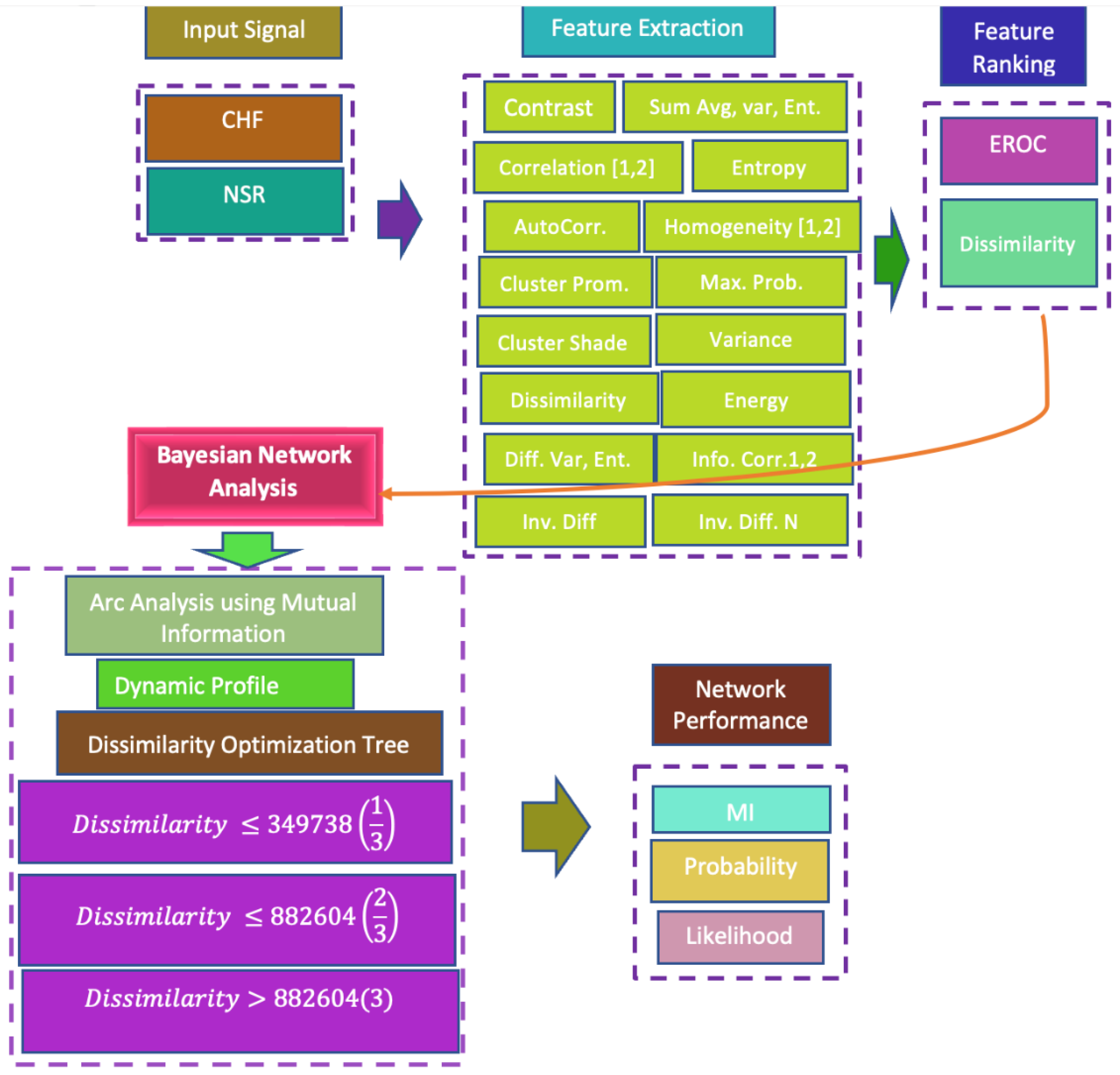
In the present era, the most common and sudden deaths occur due to cardiac and congestive heart failure (CHF). The proper and timely treatment of CHF is highly desired and demanded; researchers are therefore devising automated tools for automatic diagnosis. The dynamics produced from these signals are of a highly complex, nonlinear, and nonstationary nature. Recently, researchers have mostly utilized classification methods to distinguish the CHF from NSR. However, this study was specifically designed to first extract the GLCM features from CHF and NSR subjects, in order to capture these dynamics. We then ranked the features to determine the features’ importance, based on an empirical receiver operating characteristics (EROC) curve and random classifier slope. Finally, we utilized the robust Bayesian inference approach to determine the associations between the extracted GLCM features by computing arc analysis using mutual information, the significance of a cluster’s prominence, and overall analysis of highly ranked dissimilarity features among other extracted features. The proposed approach will further elucidate the underlying dynamics of highly complex heart variability signals, and can be used for better diagnosis and prognosis by health professionals and cardiologists for timely treatment. The associations and strengths of these relationships will be useful for further micro-level analysis and determining the significance of these features among all computed features.

The first section of the paper describes the background of the problem, the existing methods utilized and their limitations, and the proposed innovative methods. The second section explains the dataset used, feature extraction and ranking methods, the Bayesian inference methods used, along with exploratory analysis of unsupervised network analysis. The next section describes and interprets the results, and the last section discusses the main findings and limitations of this study, and future research directions.

2. Materials and Methods

2.1. Dataset

This dataset is taken from publicly available Physionet database [23]. We identified the congestive heart failure (CHF) and normal sinus rhythm (NSR) of our subjects [23]. A total of 72 subjects, including 37 women and 35 men (54 from the RR-interval NSR database and 18 from the MIT BIT normal NSR database), underwent 24 h Holter monitor recordings. The average age of the groups was 54.6 ± 16.2 (mean ± SD), ranging between 20 and 78 years. A value of 128 Hz was used to sample the ECG data. The data of CHF subjects comprised 44 subjects, including 15 women and 29 men, aged 55.5 ± 11.4, with a range of 22–78 years. We used 20,000 samples for all subjects, including both NSR and CHF subjects.

2.2. Features Extraction

In machine learning, the most important step is to extract the most relevant features. In the past, researchers [24] and [25] computed various hybrid and geometric features for colon cancer detection. The researchers [26] computed texture features to predict breast cancer. The researchers [27,28,29,30,31,32] computed various features based on texture, morphology, scale invariant feature transform (SIFT), and elliptic Fourier descriptors (EFDs) to predict brain tumors, lung cancer, breast cancer, and prostate cancer. In this study, we extracted Gray-level co-occurrence matrix (GLCM) features and then ranked the features based on empirical receiver operating characteristic (EROC) and a random classifier slope, as utilized in [33,34,35] to rank the features’ importance.

2.3. Gray-Level Co-Occurrence Matrix (GLCM)

The GLCM features are based on textural features identified by performing transitions on two pixels with a gray level technique. GLCM features were originally proposed by [36] in 1973, in a study that characterizes texture using different quantities obtained from second order image statistics. Two steps are used in obtaining GLCM features. In the first step, the pair-wise spatial co-occurrences of image pixels separated by distance d in a particular direction and angle θ are computed. The spatial relationship between the two pixels is created, i.e., the neighboring pixel and the reference pixel. In the second step, the GLCM matrix is used for computing scalar quantities which are utilized in the characterization of several aspects of an image [36]. The detailed description and mathematical formulation are described in [32,37,38,39].

2.4. Feature Ranking Algorithms

After extracting the features, all features are not equally important. The feature importance was computed using supervised feature ranking algorithms [40]. The feature importance ranking (FIR) algorithm was developed in MATLAB [41]. The importance of the computed features was measured using an empirical receiver operating characteristic (EROC) curve and a random classifier slope. The greater the ROC value indicate the more important feature.

2.5. Bayesian Inference Approach

The Bayesian approach is used to determine the association among the nodes, and is based on Bayes theorem. The Bayesian inference approach provides many comprehensive tools for in-depth analysis of the extracted nodes (features). This approach uses mutual information methods to provide the arc analysis, i.e., the strength of relationship among the nodes and association among the nodes. The optimization tree based on the selected target ‘dissimilarity’ yielded the tree with a parent–child nodes relationship, by determining importance based on the probability and joint probability scores based on the parent–child relationship. Moreover, ingoing, outgoing, and total force was computed, which helped to determine the force effect of the computed nodes.

The causal effects and their relationships are determined using a Bayesian inference approach with a directed acyclic graph (DAG) [42]. Considering X = {X₁, X₂, X₃, …, X_n} a set of n dimensional variables, the Bayesian network is defined with couplet $X=\langle G,P\rangle$ represented in angular brackets, where G denotes the DAG and P denotes the set of parameters that quantify the network that contains the probabilities of each possible value of x_i for each variable X_i. Mathematically:

$$P\left(X\right)=P\left(X_1, X_2, X_3,\dots , X_n\right)={{\displaystyle \prod }}_{i=1}^{n}P(\frac{X_i}{X_{j\left(i\right)}})$$

(1)

Here, $X_{j\left(i\right)}$ represents the set of parent variables of $X_i$ for direct acyclic graph G. This algorithm thus consequently computes the posterior probability through inference of variables of interest. BayesiaLab V10 was used for this analysis [43], by applying a set of supervised learning algorithms to search the optimal model. The Shannon entropy [44] was computed using:

$$H\left(X\right)=-{{\displaystyle \sum }}_{xϵX}p\left(X\right)lo{g}_{2}p\left(X\right)$$

(2)

2.6. Mutual Information (MI)

In this study, we utilized mutual information (MI) to compute the correlation of and strength of relationship between the extracted GLCM features from congestive heart failure signals. The mutual information algorithm computed the difference between the marginal entropy of the target variable and the conditional entropy of predicted variable, [44] denoted by MI, mathematically:

$$MI\left(X,Y\right)=H\left(X\right)-H(\frac{X}{Y})$$

(3)

MI is thus the reduction in uncertainty about the variable X, or can be the reduction in the number of X (Yes) or Y (No) questions required to guess X after observing Y. By combining H(X) and $H\left(\frac{X}{Y}\right),$ we acquire:

$$MI\left(X,Y\right)={{\displaystyle \sum }}_{xϵX}{{\displaystyle \sum }}_{yϵX}p\left(X,Y\right){ \log }_2\frac{p\left(X,Y\right)}{p\left(X\right)p\left(Y\right)}$$

(4)

Moreover, conditional mutual information (CMI) is defined as:

$$CMI\left(X,Y|Z\right)={{\displaystyle \sum }}_{xϵX}{{\displaystyle \sum }}_{yϵX}{{\displaystyle \sum }}_{y|zϵX}p\left(X,Y|Z\right){ \log }_2\frac{p(X,Y|Z)}{p\left(X|Z\right)p(Y|Z)}$$

(5)

p (X,Y) shows the joint probability distribution of X and Y, whereas p(X) and p(Y) indicate the marginal distribution of X and Y, respectively. The relevant Gaussian distribution of co-variance matrix variables X₁, X₂, X₃, …. X_n [45] can be computed as:

$$H\left(X\right)=\log {\left(2\pi e\right)}^{\frac{n}{2}}{\left|C\right|}^{\frac{-1}{2}}$$

(6)

By applying the mathematical transformation function, the MI can be calculated using following formulae:

$$MI\left(X,Y\right)=\frac{1}{2}\log \frac{\left|C\left(X\right)|\times |C\left(X\right)\right|}{\left|C\left(X,Y\right)\right|}$$

(7)

2.7. Exploratory Analysis of the Unsupervised Network

By constructing an unsupervised Bayesian network, the potential relationships between variables can be computed and explored in reality by transferring them to the model [46]. Thus, we can investigate the global analysis of the problem by computing the mutual influence of the nodes and understanding the individual influence of the variables under consideration. We built the network model using the EQ algorithm in BayesiaLab V.12 [47]. This learning method explores the space of equivalence classes of Bayesian network structures. Moreover, this method is also highly efficient, as it reduces the size of the search space to partially directed acyclic graphs (PD AGs), which are smaller than the space of Bayesian networks (DAGs), by representing equivalence classes, evaluated during each search, by computing their scores directly. A maximum weighted spanning tree (MWST) was tested. A lowest minimum description length (MDL) value was obtained with EQ, indicating the best trade-off between complexity and data representation, and validating its adoption in this study.

The Schematic flow of our model is reflected in Figure 1. We computed the GLCM texture features proposed by Avinash Uppuluri publicly available at (https://www.mathworks.com/matlabcentral/fileexchange/22187-glcm-texture-features, accessed on 20 June 2022). The description of features is mentioned in the available code i.e. 1 features taken by author from MATLAB and 2 features taken by author from the paper. The Bayesian approach has recently gained popularity and is utilized in many medical, signal, and image-processing problems. Classifying congestive heart failure is a complex problem which requires lots of effort in developing automated tools. To consider the diverse dynamics, we first computed the gray-level co-occurrence matrix (GLCM) features from the CHF and NSR subjects. We then ranked these features based on ROC values. The dissimilarity feature yielded the highest entropy values, indicating highly important features. We then set the dissimilarity feature as the target variable and applied a Bayesian approach in our further deeper analysis, which was based on four different clusters states.

Afterwards, we computed the posterior probabilities, likelihood, optimization tree, prior and posterior means, the association of the target variable with other nodes, and the detailed analysis of target node. This analysis provides a comprehensive overview of the extracted features, and their contribution and association among the nodes.

3. Results and Discussion

In this study, we first computed the GLCM features from heart failure signals. We determined these features based on ROC values. The highly important dissimilarity value was selected as our target node, and its association with other extracted target variables was computed. The detailed analysis will help to elucidate further dynamics of our complex analysis for a deeper understanding of the extracted features.

We first extracted the GLCM features from pituitary and meningioma brain MRI images. We then ranked the features based on entropy values. The ranked values, based on entropy, are shown in Figure 2. The importance of the features based on entropy value are energy (3.069), hoomogenity1 (2.7317), homogenity2 (2.6927), maximum probability (2.6818), and so on. We then chose energy as the target variable to compute its association with other computed GLCM features using a Bayesian inference approach.

Figure 3 shows the arc analysis using the MI method. The arcs between the nodes show the strength of the relationship between the nodes. The bolder arc with greater values shows the highest strength between the nodes; the arc line decreases accordingly as the value and strength of the relationship decreases. There are also other methods for computing arc analysis, including Pearson’s correlation (PC), etc. However, in the present study, we only utilized the MI for our arc analysis. Moreover, node size can be computed using different methods, including mean, normalized mean value, node force, etc., to reflect the node size. However, in this study, the node size was computed using the normalized mean value.

In this study, we computed the GLCM features and computed the associations among them using mutual information, as reflected in Figure 3. The arcs show the strengths of relation, and the nodes show the normalized mean values. The relationship of the highest strength was yielded by $\mathrm{correlation}\to \mathrm{correlation}1,1.4640,$ followed by $\mathrm{dissimilarity}\to \mathrm{homogenity}1,1.2164$, $\mathrm{energy}\to \mathrm{entropy},1.0845$, and so on.

Table 1. Node force of extracted GLCM features from congestive heart failure signals.

Node	Outgoing Force	Incoming Force	Total Force
Dissimilarity	0.9330	1.0146	1.9477
Cluster prominance	1.6428	0.0000	1.6428
Contrast	0.5446	0.6281	1.1727
Cluster shade	0.0000	0.9330	0.9330
Correlation	0.5954	0.2848	0.8802
Energy	0.5824	0.2278	0.8102
Entropy	0.1956	0.5824	0.7779
Autocorrelation	0.2848	0.3167	0.6015
Correlation2	0.0000	0.5954	0.5954
Homogenity1	0.0000	0.1956	0.1956

shows the outgoing, incoming, and total force of extracted GLCM features from congestive heart failure signals. The highest incoming force was yielded at node dissimilarity (1.0146), outgoing force (0.9330), and total force (1.9477), followed by cluster shade with incoming force (0.9330), outgoing force (0.000), and total force (0.9330); this contrasts with incoming force (0.6281), outgoing force (0.5446), and total force (1.1727), and so on.

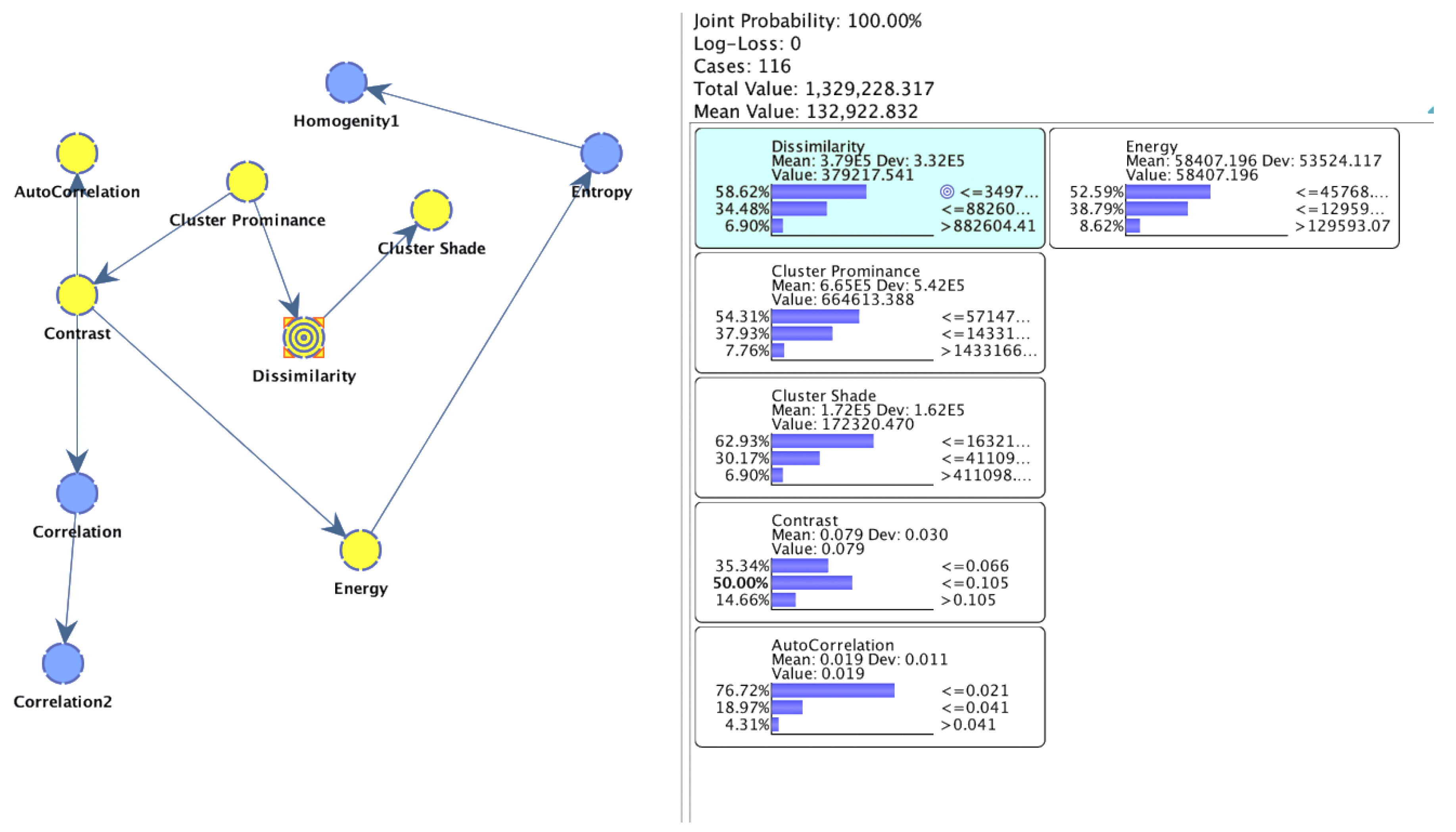
The target node of dissimilarity had a probability of 58.62% and a joint probability of 100%. The first level of the tree contains child nodes with probabilities such as cluster prominence (100%), contrast (100%), cluster shade (91.78%), energy (73.53%), entropy (68.23%), homogenity1 (68.23%), autocorrelation (67.79%), correlation (63.95%), and correlation1 (62.51%). The red colors show the 1/3rd cluster, green shows the 3/3rd cluster ranges. Navy blue color denote the probabilities at each node. Light purple denotes the joint probability and white denote the scores as reflected in Figure 4.

At the second level, cluster shades produce child nodes with probabilities such as energy (95.38%), entropy (94.21%), homogenity1 (94.21%), autocorrelation (93.56%), correlation (92.91%), and correlation1 (92.64%). Likewise, energy has child nodes of autocorrelation, correlation, and correlation2. Moreover, homogeneity1 has child nodes of autocorrelation, correlation, and correlation2. At the third level, energy, entropy, and homogenity1 have the child nodes autocorrelation, correlation, and correlation2.

Figure 5 shows the unsupervised clustering when dissimilarity was the selected target node. The arrows indicate the direction of relationship. Further dynamics are computed based on the target node’s associations with other nodes. The right part of the figure indicates the different cluster states with their occurrence out of the total subjects.

Figure 6 shows the significance of the selected top ranked dissimilarity node with other nodes such as cluster prominence, cluster shade, contrast, autocorrelation, energy, entropy, correlation, correlation2, and homogeinity1. The highest association was yielded in the cluster ≤349,738 (58.62%) with the red lines showing cluster prominence, contrast, and cluster shade with probability in the range of 0.0 to 1.0, and with other nodes in the range 0.3 to 0.75. The second highest occurrence of dissimilarity was yielded in the cluster ≤882,604 (34.48%), indicated in the green color, with cluster prominence and cluster shades occurring in the highest probability range of 0.0 to 0.90.

Table 2. Overall analysis of the highly ranked feature $\text{“}\mathrm{dissimilarity}\text{”}$ (target feature) with other extracted features.

Node	Mutual Information (MI)	Normalized MI	Relative MI	Relative Significance	p-Value
Cluster prominence	1.0146	64.01%	81.33%	1.0000	0.0000
Cluster shade	0.9330	58.86%	74.79%	0.9196	0.0000
Contrast	0.5425	34.22%	43.48%	0.5347	0.0000
Autocorrelation	0.1329	8.38%	10.65%	0.1310	0.00026
Energy	0.0895	5.64%	7.17%	0.0882	0.006164
Entropy	0.0519	3.72%	4.16%	0.0512	0.0795
Correlation	0.0394	2.48%	3.15%	0.0388	0.176
Correlation2	0.0291	1.83%	2.33%	0.0287	0.3218
Homogenity1	0.0118	0.74%	0.94%	0.0116	0.7549

shows the overall analysis of the high-ranked feature of dissimilarity as the target node, alongside other nodes. The highest performance was yielded using cluster prominence with mutual information (MI) as 1.0146, normalized MI (64.01%), relative MI (81.33%), and relative significance (1.000), followed by cluster shade, contrast, autocorrelation, energy, entropy, correlation, correlation2, and homogeneity.

Table 3. Local analysis with target states $\mathrm{dissimilarity} \le 349,738.09\left(\frac{1}{3}\right)58.62\%$.

Node	Binary MI	Relative Binary Significance	Binary Relative Significance	Maximum Bayes Factor
Cluster prominence	0.7847	80.19%	1.000	≤571,475 (1/3)	92.64%	1.7059
Cluster shade	0.6640	67.86%	0.8462	≤163,215 (1/3)	98.52%	1.5657
Contrast	0.3957	40.44%	0.5043	≤0.068 (1/3)	60.29%	1.7059
Autocorrelation	0.0839	8.57%	0.1069	≤0.021 (1/3)	88.73%	1.1566
Energy	0.0802	8.19%	0.1021	≤45,768 (1/3)	65.96%	1.2544
Entropy	0.0481	4.92%	0.0614	≤57,145 (1/3)	73.25%	1.1640
Correlation	0.0279	2.85%	0.0356	≤0.041 (1/3)	80.88%	1.0910
Correlation2	0.0215	2.19%	0.0274	≤0.058 (1/3)	87.33%	1.0664
Homogenity1	0.0112	1.14%	0.0143	>2.201 (1/3)	9.03%	1.1640

shows the local analysis for cluster 1 of 3. The highest significance was yielded with cluster prominence with binary MI (0.7847), relative binary significance, (80.19%), binary relative significance (1.000), and max. Bayes factor (92.64%), followed by cluster shade, contrast, and so on.

Table 4. Local analysis with target states $\mathrm{dissimilarity} \le 882,604.41\left(\frac{2}{3}\right)34.48\%$.

Node	Binary MI	Relative Binary Significance	Binary Relative Significance	Maximum Bayes Factor
Cluster prominence	0.6966	74.95%	1.000	≤1,433,166.15 (2/3)	97.50%	2.5705
Cluster shade	0.6150	66.17%	0.84828	≤411,098.14 (2/3)	85.00%	2.8171
Contrast	0.2993	32.20%	0.4297	≤0.105 (2/3)	84.20%	1.6841
Energy	0.0441	4.74%	0.0633	>129,593.07 (2/3)	11.90%	1.3809
Entropy	0.0259	2.78%	0.0372	>156,446.10 (3/3)	5.92%	1.3751
Autocorrelation	0.0160	1.71%	0.0229	>0.041 (3/3)	6.73%	1.5628
Correlation	0.0069	0.74%	0.0100	>0.089 (2/3)	13.01%	1.3722
Homogenity1	0.0063	0.67%	0.0090	≤1.241 (1/3)	56.32	1.1265
Correlation2	0.0055	0.58%	0.0078	>0.124 (3/3)	8.28%	1.3722

shows the local analysis for cluster 2 of 3. The highest significance was yielded with cluster prominence with binary MI (0.6966), relative binary significance (74.95%), binary relative significance (1.000), and max. Bayes factor (97.50%), followed by cluster shade, contrast, and so on.

Table 5. Local analysis with target states $\mathrm{dissimilarity} \ge 882,604.41\left(\frac{3}{3}\right)6.89\%$.

Node	Binary MI	Relative Binary Significance	Binary Relative Significance	Maximum Bayes Factor
Cluster shade	0.3621	100%	1.000	>411,098 (3/3)	100%	14.500
Cluster prominence	0.3230	89.21%	0.8922	>1,433,166 (3/3)	100%	12.888
Contrast	0.2159	59.62%	0.5962	>0.105 (3/3)	100%	6.8235
Autocorrelation	0.0907	25.06%	0.2506	≤0.041 (2/3)	76.47%	4.032
Energy	0.0287	7.94%	0.0794	>129,593 (3/3)	29.41%	3.411
Correlation	0.0241	6.65%	0.0665	>0.089 (3/3)	25.75%	2.716
Correlation2	0.0171	4.73%	0.0473	>0.124 (3/3)	16.39%	2.716
Entropy	0.0154	4.25%	0.0426	>156,446 (3/3)	12.81%	2.972
Homogenity1	0.0033	0.90%	0.0090	≤1.241 (1/3)	62.03%	1.240

shows the local analysis for cluster 3 of 3. The highest significance was yielded with cluster prominence with binary MI (0.3621), relative binary significance (100%), binary relative significance (1.000), and max. Bayes factor (100%), followed by cluster shade, contrast, and so on.

Recently, the need has arisen for a comprehensive analysis to compute the associations among the computed features, in order to understand the strength of relationships, associations, the incoming and outgoing forces between parent and child nodes, and the significance of target nodes and target nodes trees; this analysis can be carried out using the robust Bayesian inference approach. This approach will further help us to determine the underlying dynamics and relationships among the extracted nodes, which will help the relevant healthcare professionals to further improve their decision-making capabilities and diagnostic procedures. Hussain et al. [28] extracted the morphological features from prostate cancer data, in order to compute the associations between these features for deeper analysis.

4. Conclusions

The dynamics of heart signals are highly complex and nonlinear in nature. To explicate these nonlinear dynamics, we first computed the gray level co-occurrence matrix (GLCM) features to capture these dynamics. We ranked the extracted features based on EROC to determine their importance. The dissimilarity feature yielded the highest EROC value (0.3589), followed by inverse difference (0.3564), cluster prominence (0.3441), and so on. We computed the association and strength of relationships among these features using mutual information (MI). The nodes $\mathrm{correlation}\to \mathrm{correlation}1 \left(1.4640\right)$ yielded the relationship with the highest strength. We then selected dissimilarity as the target node and computed the significance with other selected states. Finally, we computed the local analysis of dissimilarity at selected states by computing binary mutual information, relative binary significance, and the maximum Bayes factor to further clarify the underlying nonlinear dynamics. The results reveal that the proposed method is more robust as a means of determining the nonlinear dynamics of heart failure signals and will lead to further improvement in prognosis and diagnosis. Currently, we have tested the results on a small dataset with no clinical profiles available. In future, we will test on larger datasets with more clinical details, which present congestive heart failure data and other demographic information. We will also apply more in-depth Bayesian inference analysis to further explain the nonlinear dynamics present in these datasets, to further improve healthcare professionals’ decision making and diagnostic capabilities.