Abstract
Deep learning (DL), often called artificial intelligence (AI), has been increasingly used in Pathology thanks to the use of scanners to digitize slides which allow us to visualize them on monitors and process them with AI algorithms. Many articles have focused on DL applied to prostate cancer (PCa). This systematic review explains the DL applications and their performances for PCa in digital pathology. Article research was performed using PubMed and Embase to collect relevant articles. A Risk of Bias (RoB) was assessed with an adaptation of the QUADAS-2 tool. Out of the 77 included studies, eight focused on pre-processing tasks such as quality assessment or staining normalization. Most articles (n = 53) focused on diagnosis tasks like cancer detection or Gleason grading. Fifteen articles focused on prediction tasks, such as recurrence prediction or genomic correlations. Best performances were reached for cancer detection with an Area Under the Curve (AUC) up to 0.99 with algorithms already available for routine diagnosis. A few biases outlined by the RoB analysis are often found in these articles, such as the lack of external validation. This review was registered on PROSPERO under CRD42023418661.
1. Introduction
1.1. Prostate Cancer
Prostate cancer (PCa) is one of the most prevalent cancers among male cancers, especially aging [1]. The gold standard for diagnosing and treating patients is the analysis of H&E histopathology slides [2]. The observation of the biopsy tissue enables pathologists to detect tumor cells and characterize the aggressiveness of the tumor using Gleason grading. This grading is based on gland structure and ranks 1 to 5 according to the differentiation [3]. When more than one pattern is present on the biopsy, the scoring is defined by the most represented pattern (primary) and the highest one (secondary). For instance, a biopsy with most of pattern 3 and some patterns 4 and 5 will be scored 3 + 5 = 8. To improve the prognosis correlation among these scores, an update of Gleason grading called the ISUP (International Society of Urological Pathology) Grading system, was proposed in 2014, which assigns patients into a group depending on the Gleason score (see Table 1) [4]. These groups have varying prognoses, from group 1 corresponding to an indolent tumor to group 5 having a poor prognosis [5].

Table 1.
Correspondence between Gleason score and ISUP Gleason group.
1.2. DL Applied to WSI
Glass slides are digitized with scanners to form whole slide images (WSIs). These images can be used to train DL algorithms. The principle is to teach an algorithm to correlate WSIs to a target provided by the user called the ground truth (GT). Once training is over, it is essential to test (or validate) the algorithm on other WSIs to validate it on other images. All studies must therefore have a training and a testing (or validation) cohort. Additionally, to comprehensively evaluate a model, it is common to use cross-validation (cross-val), i.e., splitting the training dataset into n parts, called folds, to train a model with (n − 1)/n of all data and evaluate it with 1/n of all data, n times. Finally, the algorithm can be evaluated on an external dataset.
Two main types of algorithms are discussed in this paper: segmentation and classification algorithms. Segmentation algorithms aim at precisely delineating regions of interest in WSIs (see Figure 1A). For instance, a common segmentation task is to localize stroma and epithelium. The most popular architecture is U-Net [6]. Classification algorithms intend to estimate labels, called classes, associated with images. In pathomics, WSIs are divided into tiles that are then encoded into features representing a summary of the tiles. A classification process is then learned from the features (see Figure 1B). These features are deep-learned with convolutional neural networks (CNN). The main architectures that are used for classification are Inception [7], ResNet [8], VGG [9], DenseNet [10], and MobileNet [11]. Those classic architectures can be trained and customized, but it is also possible to use models pre-trained on other data and fine-tune these models on the desired data. This is called transfer learning.
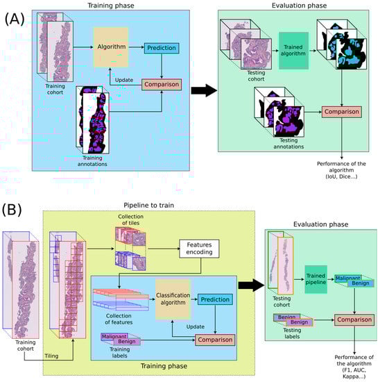
Figure 1.
DL applied to WSIs. (A) Segmentation algorithm, (B) Classification algorithm. WSIs are divided into many tiles, and every tile is encoded into features. Tiling can be performed at different magnifications, but an identical number of tiles per WSIs is generally required. The encoding into features can be trained or performed with a pre-trained algorithm. Features are then used to train a classification algorithm.
A significant difficulty in pathomics is the very large size of WSIs which prevents them from being processed all at once. This requires tiling WSIs in many tiles and dealing with data of different sizes. Most architectures need the same size of input for every image. The number of tiles selected must therefore be the same for each image. The magnification at which the image is tiled is also a key parameter in handling the input data. Additionally, this leads to potentially very large amounts of data to manually annotate to create the GT, a time-consuming task for pathologists. Strategies such as weak supervision, where only one label per patient is assigned from the pathologists’ report, have emerged to speed up this work.
1.3. Applications and Evaluation of Algorithms
In pathomics applied to PCa, DL algorithms are applied for pre-processing, diagnosis, or prediction. Pre-processing algorithms evaluate input data quality and staining normalization. Diagnosis methods focus either on cancer detection or on Gleason grading. Prediction approaches focus on predicting survival and cancer progression or genomic signatures. Algorithms are evaluated with different metrics that are summarized in Supplementary Table S1. The most used metric is the Area Under the Curve (AUC) which can be used to evaluate diagnosis and prognosis tasks.
1.4. Aim of This Review
This paper reviews the main articles mentioning DL algorithms applied to prostate cancer WSIs until 2022. It highlights current trends, future perspectives, and potential improvements in the field. It aims to be a thorough but comprehensive take on this subject for everyone interested.
2. Materials and Methods
This systematic review followed the PRISMA guidelines, containing advices and checklists to frame systematic reviews [12]. It was registered on PROSPERO, a website identifying all existing and undergoing systematic reviews under CRD42023418661.
PubMed and Embase, two biomedical databases, were used to look for articles until 1 September 2023 with the following keywords:
(‘prostate’ OR prostate OR prostatic) AND (cancer OR carcinoma OR malignant OR lesions) AND (‘artificial intelligence’ OR ‘algorithm’ OR ‘deep learning’ OR ‘machine learning’ OR ‘automated classification’ OR ‘supervised learning’ OR ‘neural network’) AND (‘whole slide image’ OR ‘digital pathology’ OR pathomics OR ‘he’ OR ‘H&E’ OR ‘histological’)
Additionally, selected papers had to:
- be written in English,
- focus on prostate cancer,
- use pathology H&E-stained images,
- rely on deep learning.
The selection of papers was first evaluated with titles only. Abstracts were then reviewed, leading to a collection of 45 selected papers. Finally, 32 articles that did not come through the database search but were referenced in many of the 45 papers were manually added. Additional searches via PubMed and Google were performed to check if conference abstracts led to published articles. Figure 2 illustrates the selection process.
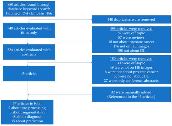
Figure 2.
Flowchart illustrating the selection process of articles in this review.
A risk-of-bias study was performed for each paper, using an adaptation of QUADAS-2 [13] (see Table 2) as the most suitable tool for AI papers. QUADAS-AI is not yet available [14]. Remarks made in this paper and criteria in the IJMEDI checklist [15] were used to create a homemade checklist adapted to this review. This allowed us to evaluate all papers on the same criteria to outline the main biases.
Table 2.
Checklist used to perform RoB analysis for every paper.
3. Results
Data was collected for every article: first author name, year of publication, aim of the paper, neural network used, number of slides in the training, validation (internal and external) cohorts, sub-aims of the paper and their corresponding performances with an Excel Sheet. All tables can be found in the Supplementary Materials with more detailed information (Supplementary Tables S2–S8).
3.1. Pre-Processing
Out of the 77 selected articles, three proposed methods for WSI quality assessment and 6 attended to correct for staining and/or scanning discrepancies across a set of WSIs (Table 3).
Table 3.
Papers focusing on pre-processing tasks.
3.1.1. Quality Assessment
Two articles proposed to evaluate the quality of a collection of slides by using a purity score (AUC of 0.8) [18] or a binary criterion of usability (AUC of 0.983) [17], attributed by pathologists. A third study proposed to artificially alter a collection of WSIs with artifacts and to evaluate the resulting impact on the tissue classification of tiles, which was perfectly performed without artifacts (F1-score = 1) [16]. The authors demonstrated that the main causes for the drop in performance are defocusing, jpg compression and staining variations. Indeed, the latter topic has been the subject of quite some articles in the field.
3.1.2. Staining Normalization and Tile Selection
WSIs stained in different locations show differences in intensity observed in the three-color channels (RGB). The scanners also influence the acquired WSIs. Many methods were proposed to normalize staining and/or scanning to obtain more generic DL models. Swiderska-Chadaj et al. evaluated the performance of their WSI normalization when classifying patients for benign/malignant tissues [24]. First, they improved classification performance with external datasets when images were scanned with the same scanner as the one used to scan the training cohort. Then, they trained a generative model to normalize WSIs for the external dataset, improving their classification performance (from an AUC of 0.92 to 0.98). Similarly, Rana et al. virtually stained with H&E non-stained WSIs with the help of generative models. Then, they stained the same biopsies with H&E and compared virtual and stained slides, reaching a high correlation (PC of 0.96) [22]. Salvi et al. focused not only on staining normalization but also on tile selection. Basing itself on segmentation, it allows for better select tiles to represent the WSI and its tissue’s complexity [25]. The model improvement (gain of 0.3 in specificity, reaching a sensitivity of 1) highlights the need for preprocessing steps, such as stain normalization or segmentation-guided tile selection.
3.2. Diagnosis
Most of the selected papers (n = 53) focused on diagnosis, whether it be about tissue segmentation (n = 5), detection of cancer tissue (n = 21), attribution of a Gleason grading (n = 10), or both detection of cancer tissue and Gleason grading (n = 19 with 2 in segmentation also). Diagnosis can be performed at the pixel level, tile level, WSI level or patient level. Methods processing data at the pixel level are segmentation algorithms trained to localize areas of clinical interest, e.g., malignant and benign epithelium. Methods processing data at tile, WSI or patient level are classification algorithms trained to identify categories of clinical interest associated with the input data.
3.2.1. Segmentation
Many segmentation studies (see Table 4) demonstrated high performance for gland segmentation: a Dice of 0.84 [26], a Dice of 0.9 [27], an F1 score from 0.83 to 0.85 [28] and an AUC of 0.99 [29]. Precisely annotating WSIs is time-consuming, and several approaches focused on strategies to reduce the number of annotations. In [30], the authors trained a model with rough annotations obtained with traditional image processing techniques. Then they fine-tuned this model with a few precise annotations made by pathologists (AUC gain of 0.04). In [28], slides were first stained with immunohistochemistry (IHC) for which DL models were already trained. The slides were stained with H&E, and a new model was trained using the annotations masks obtained from the IHC segmentation model.
Table 4.
Papers focusing on segmenting glands or tissue to help future classification tasks.
3.2.2. Cancer Detection
Even if segmentation helps select tiles of interest, other processes can be used to improve classification. There is the possibility of using multi-scale embedding to take in an area at different magnifications at the same time (as a pathologist would do) [31]. To select tiles and improve the explainability of the model, one of the most popular approaches for patient classification in pathology is Multiple Instance Learning (MIL) [32,33,34]). From a WSI divided into a high number of tiles, the goal is to associate to each tile a probability for the considered classification task, e.g., the presence of cancer, and then use the most predictive tiles to diagnose. This DL approach directly addresses the tile selection during the training, allowing us to deal with WSIs of different sizes and identify the tiles used to decide. This paradigm was notably used for cancer detection by Campanella et al. on the largest training and external validation cohorts to date [32] and by Pinckaers et al. [33]. These articles achieve an AUC of 0.99 on internal validation cohorts and above 0.90 on external cohorts. Indeed, many other approaches obtained AUC over 0.95 [31,32,33,34,35,36,37,38,39,40,41,42,43,44,45,46]. In 2021, the FDA approved the deployment of PaigeProstate [34], based on the MIL architecture of Campanella [32]. It was evaluated with three different external cohorts [47,48,49]. It showed a high performance (sensitivity of minimum 0.94 and specificity of minimum 0.93), focusing on a high sensitivity to avoid missing small areas of cancer. Other articles focused on the detection of more specific patterns, such as cribriform patterns with an accuracy of 0.88 and AUC of 0.8 [50,51,52] or perineural invasion with an AUC of 0.95 [36]. To evaluate the generalization of their model trained on biopsies for which they obtained an AUC of 0.96, Tsuneki et al. applied it to TUR-P (TransUrethral Resection of Prostate) biopsies with an AUC of 0.80. After fine-tuning their model with colon WSIs, performance on TUR-P biopsies increased to 0.85 AUC [53]. Wen fine-tuning their model with the TUR-P training cohort, they obtained an AUC of 0.9 for every testing cohort [54]. All the articles focusing on cancer detection are in Table 5.
Table 5.
Papers focusing on cancer detection only.
3.2.3. Gleason Grading
When estimating Gleason grading, many papers only focused on classifying tiles or small regions like TMAs by taking advantage of classical CNN architectures trained on large datasets of natural images such as ImageNet [60]. In that context, tiles were encoded into features which corresponded to the input data for classification [21,38,61,62,63,64,65,66]. One of the first papers in the field used a cohort of 641 TMAs, obtaining a quadratic Cohen Kappa of 0.71 [21]. Similarly, Kott et al. obtained an AUC of 0.82 [62]. A few articles directly addressed the localization at the pixel level of Gleason patterns [28,29,41,67,68,69,70,71]. Performances vary between IoU of 0.48 [70,71] to IoU around 0.7 [28,29,68], Dice score of 0.74 [69], quadratic Cohen kappa of 0.854 [41], sensitivity of 0.77 and specificity of 0.94 [67] (see Table 6). Adding epithelium detection greatly improved performance when properly segmenting areas depending on Gleason grades (gain of 0.07 in mean IoU) [29]. Many articles used the same pipeline to group Gleason scores according to ISUP recommendations [35,36,52,72,73]. These studies relied on the annotation of glands according to their Gleason pattern. WSIs were then split into tiles, and every single tile was classified according to the majority Gleason pattern (GP). Once all tiles were classified, heatmaps were generated, and a classifier was trained to properly aggregate ISUP grade groups or at least differentiate high from low grade [74]. Two algorithms based on this pipeline are now commercially available: (i) IBEX [36] (AUC of 0.99 for cancer detection, AUC of 0.94 for low/high-grade classification); (ii) DeepDx [72] (quadratic kappa of 0.90). DeepDx was further evaluated on an external cohort by Jung et al. [75] (kappa of 0.65 and quadratic kappa of 0.90). A third algorithm capable of Gleason grading (kappa of 0.77) was commercialized by Aiforia [42]. Another important milestone in the field was the organization and the release of the PANDA challenge focusing on Gleason grading at the WSI level without gland annotations [76]. This is an incredibly large cohort (around 12,000 biopsies of 3500 cases) publicly available, including slides from 2 different locations and external validation from 2 other sites. Best algorithms reached a quadratic Kappa of 0.85 on external validation datasets. One of the goals of Gleason grading algorithms is the potential decrease of inter-observer variability for pathologists using the algorithm. Some algorithms already have better Kappas than a cohort of pathologists compared to the ground truth [21,41,77].
Table 6.
Articles focusing on Gleason grading.
Table 6.
Articles focusing on Gleason grading.
| First Author, Year Reference | DL Architecture | Training Cohort | IV Cohort | EV Cohort | Aim | Results |
|---|---|---|---|---|---|---|
| Källén, 2016 [63] | OverFeat | TCGA | 10-fold cross val | 213 WSIs | GP tile classification | ACC: 0.81 |
| Classify WSIs with a majority GP | ACC: 0.89 | |||||
| Jimenez Del Toro, 2017 [74] | GoogleNet | 141 WSIs | 47 WSIs | None | High vs. Low-grade classification | ACC:0.735 |
| Arvaniti, 2018 [21] | MobileNet + classifier | 641 TMAs | 245 TMAs | None | TMA grading | qKappa: 0.71/0.75 (0.71 pathologists) |
| Tile grading | qKappa: 0.55/0.53 (0.67 pathologists) | |||||
| Poojitha, 2019 [64] | CNNs | 80 samples | 20 samples | None | GP estimation at tile level (GP 2 to 5) | F1: 0.97 |
| Nagpal, 2019 [73] | InceptionV3 | 1159 WSIs | 331 WSIs | None | GG classification | ACC: 0.7 |
| High/low-grade classification (GG 2, 3 or 4 as threshold) | : 0.95 | |||||
| Survival analysis, according to Gleason | HR: 1.38 | |||||
| Silva-Rodriguez, 2020 [52] | Custom CNN | 182 WSIs | 5-fold cross-val | 703 tiles from 641 TMAs [21] | GP at the tile level | : 0.713 (IV) & 0.57 (EV) qKappa: 0.732 (IV) & 0.64 (EV) |
| GG at the WSI level | qKappa: 0.81 (0.77 with [21] method) | |||||
| Cribriform pattern detection at the tile level | AUC: 0.822 | |||||
| Otalora, 2021 [65] | MobileNet-based CNN | 641 TMAs 255 WSIs | 245 TMAs 46 WSIs | None | GG classification | wKappa: 0.52 |
| Hammouda, 2021 [78] | CNNs | 712 WSIs | 96 WSIs | None | GP at the tile level | : 0.76 |
| GG | : 0.6 | |||||
| Marini, 2021 [66] | Custom CNN | 641 TMAs 255 WSI | 245 TMAs 46 WSIs | None | GP at the tile level | qKappa: 0.66 |
| GS at TMA level | qKappa: 0.81 | |||||
| Marron-Esquivel, 2023 [77] | DenseNet121 | 15,020 patches | 2612 patches | None | Tile-level GP classification | qKappa: 0.826 |
| 102,324 patches (PANDA + fine-tuning) | qKappa: 0.746 | |||||
| Ryu, 2019 [72] | DeepDx Prostate | 1133 WSIs | 700 WSIs | None | GG classification | qKappa: 0.907 |
| Karimi, 2019 [61] | Custom CNN | 247 TMAs | 86 TMAs | None | Malignancy detection at the tile level | Sens: 0.86 Spec: 0.85 |
| GP 3 vs. 4/5 at tile level | Sens: 0.82 Spec: 0.82 | |||||
| Nagpal, 2020 [35] | Xception | 524 WSIs | 430 WSIs | 322 WSIs | Malignancy detection at the WSI level | AUC: 0.981 Agreement: 0.943 |
| GG1-2 vs. GG3-5 | AUC: 0.972 Agreement: 0.928 | |||||
| Pantanowitz, 2020 [36] | IBEX | 549 WSIs | 2501 WSIs | 1627 WSIs | Cancer detection at the WSI level | AUC: 0.997 (IV) & 0.991 (EV) |
| Low vs. high grade (GS 6 vs. GS 7–10) | AUC: 0.941 (EV) | |||||
| GP3/4 vs. GP5 | AUC: 0.971 (EV) | |||||
| Perineural invasion detection | AUC: 0.957 (EV) | |||||
| Ström, 2020 [37] | InceptionV3 | 6935 WSIs | 1631 WSIs | 330 WSIs | Malignancy detection at the WSI level | AUC: 0.997 (IV) 0.986 (EV) |
| GG classification | Kappa: 0.62 | |||||
| Li, 2021 [39] | Weakly supervised VGG11bn | 13,115 WSIs | 7114 WSIs | 79 WSIs | Malignancy of slides | AUC: 0.982 (IV) & 0.994 (EV) |
| Low vs. high grade at the WSI level | Kappa: 0.818 Acc: 0.927 | |||||
| Kott, 2021 [62] | ResNet | 85 WSIs | 5-fold cross-val | None | Malignancy detection at the tile level | AUC: 0.83 ACC: 0.85 for fine-tuned detection |
| GP classification at the tile level | Sens: 0.83 Spec: 0.94 | |||||
| Marginean, 2021 [79] | CNN | 698 WSIs | 37 WSIs | None | Cancer area detection | Sens: 1 Spec: 0.68 |
| GG classification | : 0.6 | |||||
| Jung, 2022 [75] | DeepDx Prostate | Pre-trained | Pre-trained | 593 WSIs | Correlation with reference pathologist (pathology report comparison) | Kappa: 0.654 (0.576) qKappa: 0.904 (0.858) |
| Silva-Rodriguez, 2022 [40] | VGG16 | 252 WSIs | 98 WSIs | None | Cancer detection at the tile level | AUC: 0.979 |
| GS at the tile level | AUC: 0.899 | |||||
| GP at the tile level | : 0.65 (0.75 prev. Paper) qKappa: 0.655 | |||||
| Bulten, 2022 [76] | Evaluation of multiple algorithms (PANDA challenge) | 10,616 WSIs | 545 WSIs | 741 patients (EV1) 330 patients (EV2) | GG classification | qKappa: 0.868 (EV2) qKappa: 0.862 (EV1) |
| Li, 2018 [68] | Multi-scale U-Net | 187 tiles from 17 patients | 37 tiles from 3 patients | None | Segment Stroma, benign and malignant gland segmentation | IoU: 0.755 (0.750 classic U-Net) |
| Stroma, benign and GP 3/4 gland segmentation | IoU: 0.658 (0.644 classic U-Net) | |||||
| Li, 2019 * [29] | R-CNN | 513 WSIs | 5 fold cross val | None | Stroma, benign, low- and high-grade gland segmentation | : 0.79 (mean amongst classes) |
| Bulten, 2019 * [28] | U-Net | 62 WSIs | 40 WSIs | 20 WSIs | Benign vs. GP | IoU: 0.811 (IV) & 0.735 (EV) F1: 0.893 (IV) & 0.835 (EV) |
| Lokhande, 2020 [69] | FCN8 based on ResNet50 | 172 TMAs | 72 TMAs | None | Benign, grade 3/4/5 segmentation | Dice: 0.74 (average amongst all classes) |
| Li, 2018 [71] | Multi-Scale U-Net-based CNN | 50 patients | 20 patients | None | Contribution of EM for multi-scale U-Net improvement | : 0.35 (U-Net) : 0.49 (EM-adaptative 30%) |
| Bulten, 2020 [41] | Extended Unet | 5209 biopsies from 1033 patients | 550 biopsies from 210 patients | 886 cores | Malignancy detection at the WSI level | AUC: 0.99 (IV) & 0.98 (EV) |
| GG > 2 detection | AUC: 0.978 (IV) & 0.871 (EV) | |||||
| 100 biopsies | None | GG classification | qKappa: 0.819 (general pathologists) & 0.854 (DL on IV) & 0.71 (EV) | |||
| Hassan, 2022 [70] | ResNet50 | 18,264 WSIs | 3251 WSIs | None | Tissue segmentation for GG presence | : 0.48 : 0.375 |
| Lucas, 2019 [67] | Inception V3 | 72 WSIs | 24 WSIs | None | Malignancy detection at the pixel level | Sens: 0.90 Spec: 0.93 |
| GP3 & GP4 segmentation at pixel level | Sens: 0.77 Spec: 0.94 |
* Articles already in Table 4 for segmentation tissue performances. Double line separates classification (above) from segmentation algorithms (below). IV: Internal Validation. EV: External Validation. TMA: Tissue MicroArray. CNN: Convolutional Neural Network. GG: Gleason ISUP Group, GS: Gleason Score, GP: Gleason Pattern. AUC: Area Under the Curve. ACC: Accuracy. F1: F1-score, combination of precision and recall. IoU: Intersection over Union. q/wKappa: quadratic/weighted Cohen Kappa. Sens: Sensitivity. Spec: Specificity. implies the mean of this metric (e.g., ).
3.3. Prediction
Deep learning was also used to predict clinical outcomes such as recurrence status, survival or metastasis (n = 10, see Table 7) or to predict genomic signatures from WSIs (n = 5, see Table 8). This is the most complex task to perform as no visible phenotypes are known by pathologists to make such decisions.
3.3.1. Clinical Outcome Prediction
When focusing on recurrence, AUC around 0.8 [80,81] and Hazard Ratios (HR) above 4.8 [42,82,83] were obtained. A couple of articles studied the probability of developing metastasis [84,85]. The first article aimed to study if a patient developed lymph node metastasis after treatment [84] within undisclosed time frame, achieving an AUC of 0.69. The second article focused on distant metastasis, obtaining AUCs of 0.779 and 0.728 for 5- and 10-year metastasis. By combining image features and clinical data, the performance was improved to reach an AUC of 0.837 for 5- and 0.781 for ten years [85]. Liu et al. proposed to detect if benign slides belonged to a man who had no cancer or one who had cancer but on other biopsies and reached 0.74 AUC [86]. In any case, DL allows to establish decent survival models with HR of 1.38 for Nagpal et al. [73], 1.65 for Leo et al. [8] and 7.10 for Ren et al. [73,87,88].
Table 7.
Articles focusing on clinical outcome prediction.
Table 7.
Articles focusing on clinical outcome prediction.
| First Author, Year Reference | DL Architecture | Training Cohort | IV Cohort | EV Cohort | Aim | Results |
|---|---|---|---|---|---|---|
| Kumar, 2017 [81] | CNNs | 160 TMAs | 60 TMAs | None | Nucleus detection for tile selection | ACC: 0.89 |
| Recurrence prediction | AUC: 0.81(DL) & 0.59 (clinical data) | |||||
| Ren, 2018 [83] | AlexNet + LSTM | 271 patients | 68 patients | None | Recurrence-free survival prediction | HR: 5.73 |
| Ren, 2019 [88] | CNN + LSTM | 268 patients | 67 patients | None | Survival model | HR: 7.10 when using image features |
| Leo, 2021 [87] | Segmentation-based CNNs | 70 patients | NA | 679 patients | Cribriform pattern recognition | Pixel TPV: 0.94 Pixel TNV: 0.79 |
| Prognosis classification using cribriform area measurements | Univariable HR: 1.31 Multivariable HR: 1.66 | |||||
| Wessels, 2021 [84] | xse_ResNext34 | 118 patients | 110 patients | None | LNM prediction based on initial RP slides | AUC: 0.69 |
| Esteva, 2022 [85] | ResNet | 4524 patients | 1130 patients | None | Distant metastasis at five years (5Y) and ten years (10Y) | AUC: 0.837 (5Y) AUC: 0.781 (10Y) |
| Prostate cancer-specific survival | AUC: 0.765 | |||||
| Overall survival at ten years | AUC: 0.652 | |||||
| Pinckaers, 2022 [82] | ResNet50 | 503 patients | 182 patients | 204 patients | Univariate analysis for DL predicted biomarker evaluation | OR: 3.32 (IV) HR: 4.79 (EV) |
| Liu, 2022 [86] | 10-CNN ensemble model | 9192 benign biopsies from 1211 patients | 2851 benign biopsies from 297 patients | None | Cancer detection at the patient level | AUC: 0.727 |
| Cancer detection at patient level from benign WSIs | AUC: 0.739 | |||||
| Huang, 2022 [80] | NA | 243 patients | None | 173 patients | Recurrence prediction at three years | AUC: 0.78 |
| Sandeman, 2022 [42] | Custom CNN (AIForIA) | 331 patients | 391 patients | 126 patients | Malignant vs. benign | AUC: 0.997 |
| Grade grouping | ACC: 0.67 wKappa: 0.77 | |||||
| Outcome prediction | HR: 5.91 |
IV: Internal Validation. EV: External Validation. TMA: Tissue MicroArray. CNN: Convolutional Neural Network. RP: Radical Prostatectomies. LSTM: Long-Short Term Memory network. TMA: Tissue MicroArray. AUC: Area Under the Curve. ACC: Accuracy. wKappa: weighted Cohen Kappa. HR: Hazard Ratio. OR: Odds Ratio. TPV: True Positive Value. TNV: True Negative Value. implies the mean of this metric (e.g., ).
3.3.2. Genomic Signatures Prediction
Three groups started to work on the inference of genomic signatures from WSIs with the assumption that morphological features can predict pathway signatures [89,90,91]. These exploratory studies found correlations between RNA prediction from H&E images and RNA-seq signature expressions (PC ranging from 0.12 to 0.74). Schaumberg et al. carefully selected tiles containing tumor tissue and abnormal cells to train a classifier to predict SPOP mutations, reaching an AUC of 0.86 [92]. Dadhania et al. also used a tile-based approach to predict ERG-positive or negative mutational status, reaching around 0.8 AUC [93].
Table 8.
Articles focusing on genomic signatures prediction.
Table 8.
Articles focusing on genomic signatures prediction.
| First Author, Year Reference | DL Architecture | Training Cohort | IV Cohort | EV Cohort | Aim | Results |
|---|---|---|---|---|---|---|
| Schaumberg, 2018 [92] | ResNet50 | 177 patients | None | 152 patients | SPOP mutation prediction | AUC: 0.74 (IV) AUC: 0.86 (EV) |
| Schmauch, 2020 [89] | HE2RNA | 8725 patients (Pan-cancer) | 5-fold cross val | None | Prediction of gene signatures specific to prostate cancer | PC: 0.18 (TP63) 0.12 (KRT8 & KRT18) |
| Chelebian, 2021 [91] | CNN from [37] fine-tuned | Pre-trained ([37]) | 7 WSIs | None | Correlation between clusters identified with AI and spatial transcriptomics | No global metric |
| Dadhania, 2022 [93] | MobileNetV2 | 261 patients | 131 patients | None | ERG gene rearrangement status prediction | AUC: 0.82 to 0.85 (depending on resolution) |
| Weitz, 2022 [90] | NA | 278 patients | 92 patients | None | CCP gene expression prediction | PC: 0.527 |
| BRICD5 expression prediction | PC: 0.749 | |||||
| SPOPL expression prediction | PC: 0.526 |
IV: Internal Validation. EV: External Validation. CNN: Convolutional Neural Network. AI: Artificial Intelligence. CCP: Cell Cycle Progression. AUC: Area Under the Curve. PC: Pearson Correlation.
3.4. Risk of Bias Analysis
A Risk of Bias (RoB) analysis was performed for every article. Details are described in Supplementary Table S2. Results are summarized in Figure 3. Missing criteria were categorized as high risk, and partially addressed criteria (e.g., only half the dataset is publicly available) were considered as intermediate risk. Articles that validated existing algorithms or focused on prediction algorithms where ground truth was not defined by people were classified as Not Applicable (NA). This analysis particularly outlines the lack of publicly available code (and hyperparameters) and data. External cohorts for validation are often not addressed. More efforts could be provided for model explainability and dealing with imbalanced data. Indeed, this is a common difficulty in pathomics that biases training and evaluation.
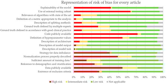
Figure 3.
Proportion of RoB for all articles. * Sufficient amount was estimated at 200 WSIs for prediction and diagnosis tasks.
4. Discussion
4.1. Summary of Results
This review article provided a systematic search following PRISMA guidelines using multiple keywords in PubMed and Embase to identify studies related to DL for PCa in pathomics. The databases and the chosen keyword might represent limitations to this systematic review. Along with breast and colorectum, prostate cancer is the organ most explored by AI. It results in a high number of publications increasing every year (see Figure 4). Among them, nine articles focused on pre-processing steps, which are key to having a robust model, namely using normalization, quality assessment and smart tile selection. It is a rather new subject (see Figure 4), and its investigation is still ongoing, with new methods to improve how input data is handled. Among the 77 articles in this review, most algorithms (n = 50) were developed for the diagnosis of cancer and the Gleason grading. There are many different algorithms, and they tend to suffer the same biases (see Supplementary Figure S1D,E). It is, therefore, harder to see what the benefits from the models are compared to the others in their respective tasks. For detection purposes, classification algorithms were more common than segmentation algorithms. The former provided heat maps giving information on the location, while the latter provided precise information at the pixel level. For the diagnosis, the AUC comprised 0.77 and 0.99 with many papers (n = 16) with AUC above 0.95, favoring the use in routine activity.
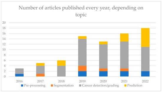
Figure 4.
Number of articles on each topic, separated by year of publication.
The most performing algorithms used the MIL paradigm, allowing some explainability, and were trained on a large number of images. Algorithms for Gleason grading were less performant, with a quadratic Cohen Kappa comprised between 0.60 and 0.90. However, the definition of ground truth in Gleason grading suffers from high inter-observer variability that renders training less reliable. The prediction was less explored, with few articles approaching the prognosis (recurrence or metastasis development, for instance) or genomic alterations, but the interest in these investigations is increasing (see Figure 4). The AUC was comprised between 0.59 and 0.86. Prediction studies aim at correlating morphological patterns to a prediction that could enable the discovery of new patterns and help in patient personalized treatment. However, more robust studies, properly designed and validated, are needed to validate this assumption.
4.2. Biases
To evaluate the biases in our review, we adapted the QUADAS-2 tool to all the studies mentioned. Several biases can be noted in the studies at the image or algorithm level. Indeed, there is no standardization on the staining protocols, which translates to WSIs. This bias could be overcome using normalization such as Vahadane [94] or Macenko methods [95] or GANs (Generative Adversarial Networks) [24] or color augmentation [32,36,61,65,66,73,96], but most articles do not use image normalization to overcome this bias (50 out of 77 do not see Figure 3). In addition, most scanners have their proprietary format, which can impair the generalizability of the algorithms. Also, the brand of the scanner impacts the scanning process, potentially decreasing algorithms’ performance when trained on different brands. It is important to develop a strategy for testing algorithms with different scanners as proposed by the UK National Pathology Imaging Co-operative (NPIC). When working on diagnosis algorithms, ground truth is biased by inter-observer variability, especially in Gleason grading studies [21,41,77]. It is important to have multiple experts provide ground-truth annotation to not follow just one pathologist’s judgement, but it is not always the case (only 32 out of 77 articles do it, Figure 3).
Furthermore, there are a few general biases in the performance evaluation of algorithms. An imbalanced dataset will induce a bias if the issue is not addressed and not all articles consider it (only 41 out of 77, Figure 3). It is possible to use only a balanced dataset or DL techniques to reduce the impact of imbalance. A model should be trained multiple times to ensure its reproducibility. The performance average of all these trainings should be considered as the performance metric of the model. However, very few articles include confidence intervals on their metrics, which are yet key to evaluating the model in the existing state of the art. Less than half the articles include external validation cohorts (24 out of 77, Figure 3), but they are necessary to ensure that the evaluated model(s) is (are) not performing well only on the training WSIs, and that is also where normalization or color augmentation during training becomes crucial.
4.3. Limits of AI
There are limitations inherent to pathomics. Contrary to radiologic images, WSI has to be divided into tiles. Most classification algorithms must have a fixed input size, generally a defined number of tiles. It means that a subset of the slide has to be selected, and the heterogeneous aspect of the tumor might not be considered. This is also affected by the choice of magnification under which the WSIs is tiled [31]. A few articles focus on new methodologies to handle this type of data [82,97]. There are also articles that suggest a smart tile selection to use more informative data and reduce computational time [25]. The particularity in PCa pathology is that the main type of images are biopsies that contain a low percentage of tissue. It can be interesting to include multiple biopsies of patients to increase the number of tiles available for training. However, the way these different biopsies are given to algorithms has to be considered. At the very least, they have to be split into the same datasets (training or testing). Otherwise, bias could be induced in the study.
Ethical regulation makes access to data difficult [98]. The existence of challenges (e.g. PANDA, Prostate cANcer graDe Assessment) is a very good way to provide data to many researchers. It also facilitates collaborations on model development. It is necessary to be able to reproduce results, which is limited by the lack of publicly available cohorts (21 out of 77 used shared data, Figure 3). However, few publications shared completely the methodology and their code with consequences on the reproducibility of the model, hindering a proper comparison of usefulness and improvement of new algorithms (only 15 out of 77 shared it, Figure 3). The popularity of AI in these last years has also increased the number of models and data to be compared, computed, and stored. This has an economic but also environmental cost that needs to be addressed [99]. Computational costs can be reduced by using more frugal but efficient architectures. Transfer learning can also reduce training time using previously developed and trained models that are fine-tuned to fit the studied data. The downfall is to conform to the input data format. Focusing on more efficient architectures and how to properly share methodology in the field are potential improvements to be found to develop long-term viable solutions. The focus should also be directed towards the explainability of the algorithms. If they are to be implemented in clinical setups, “blackbox” models will not be trusted by pathologists (Figure 3, 40 of 77 attempted some form of explainability).
4.4. Impact of AI in Routine Activity
Nonetheless, several AI tools are now available on the market for the diagnosis in routine activity for prostate cancer from different companies: Ibex, Paige, Deep Bio and AIFORIA, whose algorithms were recently published [36,42,49,75]. They can be approved for first or second-read applications if they are used before as a screening or after as a quality check for the pathologist diagnosis. The GalenTM Prostate from Ibex was the first to obtain CE under IVDR (In Vitro Diagnostic Medical Devices Regulation) in February 2023. The sensitivity and specificity of these products are very high when excluding slides with intermediate classification probability, also called undetermined categories. Indeed, a number of slides with undetermined categories are impacted by many parameters, such as pre-analytic conditions and the format of slides….
Consequently, performances depend on the site where the algorithms are deployed. In addition, their integration into routine activity supposes a digital workflow that is not widely available. Properly integrated into the workflow, it could help save time, but it is difficult to implement due to interoperability issues (integration in the Laboratory Information System (LIS) and the Image Management System (IMS)). An optimized integration supposes at least the automatized assignment of cases, the contextual launch, the cases prioritization, the visualization of heatmaps directly in the IMS and the integration of results directly in the report. Ethical considerations become an additional question when processing patient data, especially if sent to a cloud environment.
4.5. Multimodal Approach for Predictive Algorithms
Like other organs, the prediction of prostate cancer seems to be a more difficult question than detection. Indeed, the underlying assumption is that there exists a morphologic pattern in the images that can predict prognosis or genomic alteration. It is very likely that the answer is multifactorial and could benefit from multimodal approaches such as combining the WSI with radiologic, biological, and molecular data. The main challenge is properly combining all these data of different natures and evaluating the added value when combining them compared to the performance obtained by considering each separately.
5. Conclusions
In conclusion, DL has been widely explored in PCa, resulting in many pre-processing, diagnosis, or prediction publications. This systematic review highlights how DL could be used in this field and what significant improvements it could bring. It also included suggestions to reduce research biases in this field while outlining the inherent limits of these tools. Despite these limitations, PCa was one of the first organs to benefit from reliable AI tools that could already be used in routine activity for diagnosis purposes: cancer detection and Gleason grading… However, for predictive purposes, further studies are needed to improve the robustness of the algorithms, which could lead to more personalized treatment: prognosis, molecular alteration, etc.
Supplementary Materials
The following supporting information can be downloaded at: https://www.mdpi.com/article/10.3390/diagnostics13162676/s1, Figure S1: Representation of Risk of Bias for subsets of selected articles; Table S1: Details of risk of bias for all articles; Table S2: Metrics found in articles of the review and their definition; Tables S3–S8: Extended Table 3, Table 4, Table 5, Table 6, Table 7 and Table 8 found in this article.
Author Contributions
N.R. and S.-F.K.-J. came up with the idea of this review and conceptualized it. N.R., S.-F.K.-J., T.P. and P.A. then established a proper methodology to write this review. Articles search, data collection, bias analysis and figure creation were made by N.R.; Original drafting was written by N.R., T.P. and S.-F.K.-J.; Writing, reviewing,, and editing was performed by O.A., R.D.C., R.B., D.L., N.R.-L., Z.-e.K., R.M. and K.B. All this work was supervised by T.P. and S.-F.K.-J. All authors have read and agreed to the published version of the manuscript.
Funding
N.R. is funded by ARED PERTWIN grant, EraPerMED project. T.P. is funded by a Chan Zuckerberg Initiative DAF grant (2019-198009).
Institutional Review Board Statement
Not applicable.
Informed Consent Statement
Not applicable.
Data Availability Statement
The data presented in this study are available in the Supplementary Materials.
Conflicts of Interest
The authors declare no conflict of interest. The funders had no role in the design of the study; in the collection, analyses, or interpretation of data; in the writing of the manuscript; or in the decision to publish the results.
References
- Siegel, R.L.; Miller, K.D.; Fuchs, H.E.; Jemal, A. Cancer Statistics, 2022. CA Cancer J. Clin. 2022, 72, 7–33. [Google Scholar] [CrossRef]
- Descotes, J.-L. Diagnosis of Prostate Cancer. Asian J. Urol. 2019, 6, 129–136. [Google Scholar] [CrossRef] [PubMed]
- Epstein, J.I.; Allsbrook, W.C.; Amin, M.B.; Egevad, L.L.; ISUP Grading Committee. The 2005 International Society of Urological Pathology (ISUP) Consensus Conference on Gleason Grading of Prostatic Carcinoma. Am. J. Surg. Pathol. 2005, 29, 1228–1242. [Google Scholar] [CrossRef]
- Epstein, J.I.; Egevad, L.; Amin, M.B.; Delahunt, B.; Srigley, J.R.; Humphrey, P.A.; The Grading Committee. The 2014 International Society of Urological Pathology (ISUP) Consensus Conference on Gleason Grading of Prostatic Carcinoma: Definition of Grading Patterns and Proposal for a New Grading System. Am. J. Surg. Pathol. 2016, 40, 244. [Google Scholar] [CrossRef] [PubMed]
- Williams, I.S.; McVey, A.; Perera, S.; O’Brien, J.S.; Kostos, L.; Chen, K.; Siva, S.; Azad, A.A.; Murphy, D.G.; Kasivisvanathan, V.; et al. Modern Paradigms for Prostate Cancer Detection and Management. Med. J. Aust. 2022, 217, 424–433. [Google Scholar] [CrossRef]
- Ronneberger, O.; Fischer, P.; Brox, T. U-Net: Convolutional Networks for Biomedical Image Segmentation. In Medical Image Computing and Computer-Assisted Intervention–MICCAI 2015; Navab, N., Hornegger, J., Wells, W.M., Frangi, A.F., Eds.; Springer International Publishing: Cham, Switzerland, 2015; pp. 234–241. [Google Scholar]
- Szegedy, C.; Liu, W.; Jia, Y.; Sermanet, P.; Reed, S.; Anguelov, D.; Erhan, D.; Vanhoucke, V.; Rabinovich, A. Going Deeper with Convolutions. In Proceedings of the 2015 IEEE Conference on Computer Vision and Pattern Recognition (CVPR), Boston, MA, USA, 7–12 June 2015; pp. 1–9. [Google Scholar]
- He, K.; Zhang, X.; Ren, S.; Sun, J. Deep Residual Learning for Image Recognition. In Proceedings of the 2016 IEEE Conference on Computer Vision and Pattern Recognition (CVPR), Las Vegas, NV, USA, 27–30 June 2016; pp. 770–778. [Google Scholar]
- Simonyan, K.; Zisserman, A. Very Deep Convolutional Networks for Large-Scale Image Recognition. arXiv 2015, arXiv:1409.1556. [Google Scholar]
- Huang, G.; Liu, Z.; van der Maaten, L.; Weinberger, K.Q. Densely Connected Convolutional Networks. arXiv 2018, arXiv:1608.06993. [Google Scholar]
- Howard, A.G.; Zhu, M.; Chen, B.; Kalenichenko, D.; Wang, W.; Weyand, T.; Andreetto, M.; Adam, H. MobileNets: Efficient Convolutional Neural Networks for Mobile Vision Applications. arXiv 2017, arXiv:1704.04861. [Google Scholar]
- Page, M.J.; McKenzie, J.E.; Bossuyt, P.M.; Boutron, I.; Hoffmann, T.C.; Mulrow, C.D.; Shamseer, L.; Tetzlaff, J.M.; Akl, E.A.; Brennan, S.E.; et al. The PRISMA 2020 Statement: An Updated Guideline for Reporting Systematic Reviews. Syst. Rev. 2021, 10, 89. [Google Scholar] [CrossRef]
- Whiting, P.F.; Rutjes, A.W.S.; Westwood, M.E.; Mallett, S.; Deeks, J.J.; Reitsma, J.B.; Leeflang, M.M.G.; Sterne, J.A.C.; Bossuyt, P.M.M.; QUADAS-2 Group. QUADAS-2: A Revised Tool for the Quality Assessment of Diagnostic Accuracy Studies. Ann. Intern. Med. 2011, 155, 529–536. [Google Scholar] [CrossRef]
- Sounderajah, V.; Ashrafian, H.; Rose, S.; Shah, N.H.; Ghassemi, M.; Golub, R.; Kahn, C.E.; Esteva, A.; Karthikesalingam, A.; Mateen, B.; et al. A Quality Assessment Tool for Artificial Intelligence-Centered Diagnostic Test Accuracy Studies: QUADAS-AI. Nat. Med. 2021, 27, 1663–1665. [Google Scholar] [CrossRef]
- Cabitza, F.; Campagner, A. The IJMEDI Checklist for Assessment of Medical AI. Int. J. Med. Inform. 2021, 153. [Google Scholar] [CrossRef]
- Schömig-Markiefka, B.; Pryalukhin, A.; Hulla, W.; Bychkov, A.; Fukuoka, J.; Madabhushi, A.; Achter, V.; Nieroda, L.; Büttner, R.; Quaas, A.; et al. Quality Control Stress Test for Deep Learning-Based Diagnostic Model in Digital Pathology. Mod. Pathol. 2021, 34, 2098–2108. [Google Scholar] [CrossRef] [PubMed]
- Haghighat, M.; Browning, L.; Sirinukunwattana, K.; Malacrino, S.; Khalid Alham, N.; Colling, R.; Cui, Y.; Rakha, E.; Hamdy, F.C.; Verrill, C.; et al. Automated Quality Assessment of Large Digitised Histology Cohorts by Artificial Intelligence. Sci. Rep. 2022, 12, 5002. [Google Scholar] [CrossRef] [PubMed]
- Brendel, M.; Getseva, V.; Assaad, M.A.; Sigouros, M.; Sigaras, A.; Kane, T.; Khosravi, P.; Mosquera, J.M.; Elemento, O.; Hajirasouliha, I. Weakly-Supervised Tumor Purity Prediction from Frozen H&E Stained Slides. eBioMedicine 2022, 80, 104067. [Google Scholar] [CrossRef] [PubMed]
- Anghel, A.; Stanisavljevic, M.; Andani, S.; Papandreou, N.; Rüschoff, J.H.; Wild, P.; Gabrani, M.; Pozidis, H. A High-Performance System for Robust Stain Normalization of Whole-Slide Images in Histopathology. Front. Med. 2019, 6, 193. [Google Scholar] [CrossRef]
- Otálora, S.; Atzori, M.; Andrearczyk, V.; Khan, A.; Müller, H. Staining Invariant Features for Improving Generalization of Deep Convolutional Neural Networks in Computational Pathology. Front. Bioeng. Biotechnol. 2019, 7, 198. [Google Scholar] [CrossRef]
- Arvaniti, E.; Fricker, K.S.; Moret, M.; Rupp, N.; Hermanns, T.; Fankhauser, C.; Wey, N.; Wild, P.J.; Rüschoff, J.H.; Claassen, M. Automated Gleason Grading of Prostate Cancer Tissue Microarrays via Deep Learning. Sci. Rep. 2018, 8, 12054. [Google Scholar] [CrossRef]
- Rana, A.; Lowe, A.; Lithgow, M.; Horback, K.; Janovitz, T.; Da Silva, A.; Tsai, H.; Shanmugam, V.; Bayat, A.; Shah, P. Use of Deep Learning to Develop and Analyze Computational Hematoxylin and Eosin Staining of Prostate Core Biopsy Images for Tumor Diagnosis. JAMA Netw. Open 2020, 3, e205111. [Google Scholar] [CrossRef]
- Sethi, A.; Sha, L.; Vahadane, A.R.; Deaton, R.J.; Kumar, N.; Macias, V.; Gann, P.H. Empirical Comparison of Color Normalization Methods for Epithelial-Stromal Classification in H and E Images. J. Pathol. Inform. 2016, 7, 17. [Google Scholar] [CrossRef]
- Swiderska-Chadaj, Z.; de Bel, T.; Blanchet, L.; Baidoshvili, A.; Vossen, D.; van der Laak, J.; Litjens, G. Impact of Rescanning and Normalization on Convolutional Neural Network Performance in Multi-Center, Whole-Slide Classification of Prostate Cancer. Sci. Rep. 2020, 10, 14398. [Google Scholar] [CrossRef]
- Salvi, M.; Molinari, F.; Acharya, U.R.; Molinaro, L.; Meiburger, K.M. Impact of Stain Normalization and Patch Selection on the Performance of Convolutional Neural Networks in Histological Breast and Prostate Cancer Classification. Comput. Methods Programs Biomed. Update 2021, 1, 100004. [Google Scholar] [CrossRef]
- Ren, J.; Sadimin, E.; Foran, D.J.; Qi, X. Computer Aided Analysis of Prostate Histopathology Images to Support a Refined Gleason Grading System. In Proceedings of the Medical Imaging 2017: Image Processing, Orlando, FL, USA, 24 February 2017; Volume 10133, pp. 532–539. [Google Scholar]
- Salvi, M.; Bosco, M.; Molinaro, L.; Gambella, A.; Papotti, M.; Acharya, U.R.; Molinari, F. A Hybrid Deep Learning Approach for Gland Segmentation in Prostate Histopathological Images. Artif. Intell. Med. 2021, 115, 102076. [Google Scholar] [CrossRef] [PubMed]
- Bulten, W.; Bándi, P.; Hoven, J.; van de Loo, R.; Lotz, J.; Weiss, N.; van der Laak, J.; van Ginneken, B.; Hulsbergen-van de Kaa, C.; Litjens, G. Epithelium Segmentation Using Deep Learning in H&E-Stained Prostate Specimens with Immunohistochemistry as Reference Standard. Sci. Rep. 2019, 9, 864. [Google Scholar] [CrossRef] [PubMed]
- Li, W.; Li, J.; Sarma, K.V.; Ho, K.C.; Shen, S.; Knudsen, B.S.; Gertych, A.; Arnold, C.W. Path R-CNN for Prostate Cancer Diagnosis and Gleason Grading of Histological Images. IEEE Trans. Med. Imaging 2019, 38, 945–954. [Google Scholar] [CrossRef]
- Bukowy, J.D.; Foss, H.; McGarry, S.D.; Lowman, A.K.; Hurrell, S.L.; Iczkowski, K.A.; Banerjee, A.; Bobholz, S.A.; Barrington, A.; Dayton, A.; et al. Accurate Segmentation of Prostate Cancer Histomorphometric Features Using a Weakly Supervised Convolutional Neural Network. J. Med. Imaging 2020, 7, 057501. [Google Scholar] [CrossRef]
- Duong, Q.D.; Vu, D.Q.; Lee, D.; Hewitt, S.M.; Kim, K.; Kwak, J.T. Scale Embedding Shared Neural Networks for Multiscale Histological Analysis of Prostate Cancer. In Proceedings of the Medical Imaging 2019: Digital Pathology, San Diego, CA, USA, 18 March 2019; Volume 10956, pp. 15–20. [Google Scholar] [CrossRef]
- Campanella, G.; Hanna, M.G.; Geneslaw, L.; Miraflor, A.; Werneck Krauss Silva, V.; Busam, K.J.; Brogi, E.; Reuter, V.E.; Klimstra, D.S.; Fuchs, T.J. Clinical-Grade Computational Pathology Using Weakly Supervised Deep Learning on Whole Slide Images. Nat. Med. 2019, 25, 1301–1309. [Google Scholar] [CrossRef] [PubMed]
- Pinckaers, H.; Bulten, W.; van der Laak, J.; Litjens, G. Detection of Prostate Cancer in Whole-Slide Images Through End-to-End Training With Image-Level Labels. IEEE Trans. Med. Imaging 2021, 40, 1817–1826. [Google Scholar] [CrossRef]
- Raciti, P.; Sue, J.; Ceballos, R.; Godrich, R.; Kunz, J.D.; Kapur, S.; Reuter, V.; Grady, L.; Kanan, C.; Klimstra, D.S.; et al. Novel Artificial Intelligence System Increases the Detection of Prostate Cancer in Whole Slide Images of Core Needle Biopsies. Mod. Pathol. 2020, 33, 2058–2066. [Google Scholar] [CrossRef]
- Nagpal, K.; Foote, D.; Tan, F.; Liu, Y.; Chen, P.-H.C.; Steiner, D.F.; Manoj, N.; Olson, N.; Smith, J.L.; Mohtashamian, A.; et al. Development and Validation of a Deep Learning Algorithm for Gleason Grading of Prostate Cancer From Biopsy Specimens. JAMA Oncol. 2020, 6, 1372–1380. [Google Scholar] [CrossRef]
- Pantanowitz, L.; Quiroga-Garza, G.M.; Bien, L.; Heled, R.; Laifenfeld, D.; Linhart, C.; Sandbank, J.; Albrecht Shach, A.; Shalev, V.; Vecsler, M.; et al. An Artificial Intelligence Algorithm for Prostate Cancer Diagnosis in Whole Slide Images of Core Needle Biopsies: A Blinded Clinical Validation and Deployment Study. Lancet Digit. Health 2020, 2, e407–e416. [Google Scholar] [CrossRef] [PubMed]
- Ström, P.; Kartasalo, K.; Olsson, H.; Solorzano, L.; Delahunt, B.; Berney, D.M.; Bostwick, D.G.; Evans, A.J.; Grignon, D.J.; Humphrey, P.A.; et al. Artificial Intelligence for Diagnosis and Grading of Prostate Cancer in Biopsies: A Population-Based, Diagnostic Study. Lancet Oncol. 2020, 21, 222–232. [Google Scholar] [CrossRef] [PubMed]
- Han, W.; Johnson, C.; Gaed, M.; Gómez, J.A.; Moussa, M.; Chin, J.L.; Pautler, S.; Bauman, G.S.; Ward, A.D. Histologic Tissue Components Provide Major Cues for Machine Learning-Based Prostate Cancer Detection and Grading on Prostatectomy Specimens. Sci. Rep. 2020, 10, 9911. [Google Scholar] [CrossRef]
- Li, J.; Li, W.; Sisk, A.; Ye, H.; Wallace, W.D.; Speier, W.; Arnold, C.W. A Multi-Resolution Model for Histopathology Image Classification and Localization with Multiple Instance Learning. Comput. Biol. Med. 2021, 131, 104253. [Google Scholar] [CrossRef]
- Silva-Rodríguez, J.; Schmidt, A.; Sales, M.A.; Molina, R.; Naranjo, V. Proportion Constrained Weakly Supervised Histopathology Image Classification. Comput. Biol. Med. 2022, 147, 105714. [Google Scholar] [CrossRef]
- Bulten, W.; Pinckaers, H.; van Boven, H.; Vink, R.; de Bel, T.; van Ginneken, B.; van der Laak, J.; Hulsbergen-van de Kaa, C.; Litjens, G. Automated Deep-Learning System for Gleason Grading of Prostate Cancer Using Biopsies: A Diagnostic Study. Lancet Oncol. 2020, 21, 233–241. [Google Scholar] [CrossRef]
- Sandeman, K.; Blom, S.; Koponen, V.; Manninen, A.; Juhila, J.; Rannikko, A.; Ropponen, T.; Mirtti, T. AI Model for Prostate Biopsies Predicts Cancer Survival. Diagnostics 2022, 12, 1031. [Google Scholar] [CrossRef]
- Litjens, G.; Sánchez, C.I.; Timofeeva, N.; Hermsen, M.; Nagtegaal, I.; Kovacs, I.; Hulsbergen-van de Kaa, C.; Bult, P.; van Ginneken, B.; van der Laak, J. Deep Learning as a Tool for Increased Accuracy and Efficiency of Histopathological Diagnosis. Sci. Rep. 2016, 6, 26286. [Google Scholar] [CrossRef]
- Kwak, J.T.; Hewitt, S.M. Nuclear Architecture Analysis of Prostate Cancer via Convolutional Neural Networks. IEEE Access 2017, 5, 18526–18533. [Google Scholar] [CrossRef]
- Kwak, J.T.; Hewitt, S.M. Lumen-Based Detection of Prostate Cancer via Convolutional Neural Networks. In Proceedings of the Medical Imaging 2017: Digital Pathology, Orlando, FL, USA, 1 March 2017; Volume 10140, pp. 47–52. [Google Scholar]
- Campanella, G.; Silva, V.W.K.; Fuchs, T.J. Terabyte-Scale Deep Multiple Instance Learning for Classification and Localization in Pathology. arXiv 2018, arXiv:1805.06983. [Google Scholar]
- Raciti, P.; Sue, J.; Retamero, J.A.; Ceballos, R.; Godrich, R.; Kunz, J.D.; Casson, A.; Thiagarajan, D.; Ebrahimzadeh, Z.; Viret, J.; et al. Clinical Validation of Artificial Intelligence–Augmented Pathology Diagnosis Demonstrates Significant Gains in Diagnostic Accuracy in Prostate Cancer Detection. Arch. Pathol. Lab. Med. 2022. [Google Scholar] [CrossRef] [PubMed]
- da Silva, L.M.; Pereira, E.M.; Salles, P.G.; Godrich, R.; Ceballos, R.; Kunz, J.D.; Casson, A.; Viret, J.; Chandarlapaty, S.; Ferreira, C.G.; et al. Independent Real-world Application of a Clinical-grade Automated Prostate Cancer Detection System. J. Pathol. 2021, 254, 147–158. [Google Scholar] [CrossRef] [PubMed]
- Perincheri, S.; Levi, A.W.; Celli, R.; Gershkovich, P.; Rimm, D.; Morrow, J.S.; Rothrock, B.; Raciti, P.; Klimstra, D.; Sinard, J. An Independent Assessment of an Artificial Intelligence System for Prostate Cancer Detection Shows Strong Diagnostic Accuracy. Mod. Pathol. 2021, 34, 1588–1595. [Google Scholar] [CrossRef] [PubMed]
- Singh, M.; Kalaw, E.M.; Jie, W.; Al-Shabi, M.; Wong, C.F.; Giron, D.M.; Chong, K.-T.; Tan, M.; Zeng, Z.; Lee, H.K. Cribriform Pattern Detection in Prostate Histopathological Images Using Deep Learning Models. arXiv 2019, arXiv:1910.04030. [Google Scholar]
- Ambrosini, P.; Hollemans, E.; Kweldam, C.F.; van Leenders, G.J.L.H.; Stallinga, S.; Vos, F. Automated Detection of Cribriform Growth Patterns in Prostate Histology Images. Sci. Rep. 2020, 10, 14904. [Google Scholar] [CrossRef]
- Silva-Rodríguez, J.; Colomer, A.; Sales, M.A.; Molina, R.; Naranjo, V. Going Deeper through the Gleason Scoring Scale: An Automatic End-to-End System for Histology Prostate Grading and Cribriform Pattern Detection. Comput. Methods Programs Biomed. 2020, 195, 105637. [Google Scholar] [CrossRef] [PubMed]
- Tsuneki, M.; Abe, M.; Kanavati, F. A Deep Learning Model for Prostate Adenocarcinoma Classification in Needle Biopsy Whole-Slide Images Using Transfer Learning. Diagnostics 2022, 12, 768. [Google Scholar] [CrossRef]
- Tsuneki, M.; Abe, M.; Kanavati, F. Transfer Learning for Adenocarcinoma Classifications in the Transurethral Resection of Prostate Whole-Slide Images. Cancers 2022, 14, 4744. [Google Scholar] [CrossRef]
- García, G.; Colomer, A.; Naranjo, V. First-Stage Prostate Cancer Identification on Histopathological Images: Hand-Driven versus Automatic Learning. Entropy 2019, 21, 356. [Google Scholar] [CrossRef]
- Jones, A.D.; Graff, J.P.; Darrow, M.; Borowsky, A.; Olson, K.A.; Gandour-Edwards, R.; Mitra, A.D.; Wei, D.; Gao, G.; Durbin-Johnson, B.; et al. Impact of Pre-Analytic Variables on Deep Learning Accuracy in Histopathology. Histopathology 2019, 75, 39–53. [Google Scholar] [CrossRef]
- Bukhari, S.U.; Mehtab, U.; Hussain, S.; Syed, A.; Armaghan, S.; Shah, S. The Assessment of Deep Learning Computer Vision Algorithms for the Diagnosis of Prostatic Adenocarcinoma. Ann. Clin. Anal. Med. 2021, 12 (Suppl. 1), S31–S34. [Google Scholar] [CrossRef]
- Krajňanský, V.; Gallo, M.; Nenutil, R.; Němeček, M.; Holub, P.; Brázdil, T. Shedding Light on the Black Box of a Neural Network Used to Detect Prostate Cancer in Whole Slide Images by Occlusion-Based Explainability. bioRxiv 2022. [Google Scholar] [CrossRef]
- Chen, C.-M.; Huang, Y.-S.; Fang, P.-W.; Liang, C.-W.; Chang, R.-F. A Computer-Aided Diagnosis System for Differentiation and Delineation of Malignant Regions on Whole-Slide Prostate Histopathology Image Using Spatial Statistics and Multidimensional DenseNet. Med. Phys. 2020, 47, 1021–1033. [Google Scholar] [CrossRef]
- Russakovsky, O.; Deng, J.; Su, H.; Krause, J.; Satheesh, S.; Ma, S.; Huang, Z.; Karpathy, A.; Khosla, A.; Bernstein, M.; et al. ImageNet Large Scale Visual Recognition Challenge. Int. J. Comput. Vis. 2015, 115, 211–252. [Google Scholar] [CrossRef]
- Karimi, D.; Nir, G.; Fazli, L.; Black, P.C.; Goldenberg, L.; Salcudean, S.E. Deep Learning-Based Gleason Grading of Prostate Cancer From Histopathology Images—Role of Multiscale Decision Aggregation and Data Augmentation. IEEE J. Biomed. Health Inform. 2020, 24, 1413–1426. [Google Scholar] [CrossRef] [PubMed]
- Kott, O.; Linsley, D.; Amin, A.; Karagounis, A.; Jeffers, C.; Golijanin, D.; Serre, T.; Gershman, B. Development of a Deep Learning Algorithm for the Histopathologic Diagnosis and Gleason Grading of Prostate Cancer Biopsies: A Pilot Study. Eur. Urol. Focus 2021, 7, 347–351. [Google Scholar] [CrossRef]
- Kallen, H.; Molin, J.; Heyden, A.; Lundstrom, C.; Astrom, K. Towards Grading Gleason Score Using Generically Trained Deep Convolutional Neural Networks. In Proceedings of the 2016 IEEE 13th International Symposium on Biomedical Imaging (ISBI), Prague, Czech Republic, 13–16 April 2016; pp. 1163–1167. [Google Scholar]
- Poojitha, U.P.; Lal Sharma, S. Hybrid Unified Deep Learning Network for Highly Precise Gleason Grading of Prostate Cancer. Annu. Int. Conf. IEEE Eng. Med. Biol. Soc. 2019, 2019, 899–903. [Google Scholar] [CrossRef] [PubMed]
- Otálora, S.; Marini, N.; Müller, H.; Atzori, M. Combining Weakly and Strongly Supervised Learning Improves Strong Supervision in Gleason Pattern Classification. BMC Med. Imaging 2021, 21, 77. [Google Scholar] [CrossRef]
- Marini, N.; Otálora, S.; Müller, H.; Atzori, M. Semi-Supervised Training of Deep Convolutional Neural Networks with Heterogeneous Data and Few Local Annotations: An Experiment on Prostate Histopathology Image Classification. Med. Image Anal. 2021, 73, 102165. [Google Scholar] [CrossRef]
- Lucas, M.; Jansen, I.; Savci-Heijink, C.D.; Meijer, S.L.; de Boer, O.J.; van Leeuwen, T.G.; de Bruin, D.M.; Marquering, H.A. Deep Learning for Automatic Gleason Pattern Classification for Grade Group Determination of Prostate Biopsies. Virchows Arch. Int. J. Pathol. 2019, 475, 77–83. [Google Scholar] [CrossRef]
- Li, J.; Sarma, K.V.; Chung Ho, K.; Gertych, A.; Knudsen, B.S.; Arnold, C.W. A Multi-Scale U-Net for Semantic Segmentation of Histological Images from Radical Prostatectomies. AMIA Annu. Symp. Proc. AMIA Symp. 2017, 2017, 1140–1148. [Google Scholar]
- Lokhande, A.; Bonthu, S.; Singhal, N. Carcino-Net: A Deep Learning Framework for Automated Gleason Grading of Prostate Biopsies. In Proceedings of the 2020 42nd Annual International Conference of the IEEE Engineering in Medicine & Biology Society (EMBC), Montreal, QC, Canada, 20–24 July 2020; pp. 1380–1383. [Google Scholar]
- Hassan, T.; Shafay, M.; Hassan, B.; Akram, M.U.; ElBaz, A.; Werghi, N. Knowledge Distillation Driven Instance Segmentation for Grading Prostate Cancer. Comput. Biol. Med. 2022, 150, 106124. [Google Scholar] [CrossRef]
- Li, J.; Speier, W.; Ho, K.C.; Sarma, K.V.; Gertych, A.; Knudsen, B.S.; Arnold, C.W. An EM-Based Semi-Supervised Deep Learning Approach for Semantic Segmentation of Histopathological Images from Radical Prostatectomies. Comput. Med. Imaging Graph. 2018, 69, 125–133. [Google Scholar] [CrossRef] [PubMed]
- Ryu, H.S.; Jin, M.-S.; Park, J.H.; Lee, S.; Cho, J.; Oh, S.; Kwak, T.-Y.; Woo, J.I.; Mun, Y.; Kim, S.W.; et al. Automated Gleason Scoring and Tumor Quantification in Prostate Core Needle Biopsy Images Using Deep Neural Networks and Its Comparison with Pathologist-Based Assessment. Cancers 2019, 11, 1860. [Google Scholar] [CrossRef]
- Nagpal, K.; Foote, D.; Liu, Y.; Chen, P.-H.C.; Wulczyn, E.; Tan, F.; Olson, N.; Smith, J.L.; Mohtashamian, A.; Wren, J.H.; et al. Development and Validation of a Deep Learning Algorithm for Improving Gleason Scoring of Prostate Cancer. npj Digit. Med. 2019, 2, 48. [Google Scholar] [CrossRef]
- Jimenez-del-Toro, O.; Atzori, M.; Andersson, M.; Eurén, K.; Hedlund, M.; Rönnquist, P.; Müller, H. Convolutional Neural Networks for an Automatic Classification of Prostate Tissue Slides with High-Grade Gleason Score. In Proceedings of the Medical Imaging 2017: Digital Pathology, Orlando, FL, USA, 5 April 2017. [Google Scholar] [CrossRef]
- Jung, M.; Jin, M.-S.; Kim, C.; Lee, C.; Nikas, I.P.; Park, J.H.; Ryu, H.S. Artificial Intelligence System Shows Performance at the Level of Uropathologists for the Detection and Grading of Prostate Cancer in Core Needle Biopsy: An Independent External Validation Study. Mod. Pathol. 2022, 35, 1449–1457. [Google Scholar] [CrossRef] [PubMed]
- Bulten, W.; Kartasalo, K.; Chen, P.-H.C.; Ström, P.; Pinckaers, H.; Nagpal, K.; Cai, Y.; Steiner, D.F.; van Boven, H.; Vink, R.; et al. Artificial Intelligence for Diagnosis and Gleason Grading of Prostate Cancer: The PANDA Challenge. Nat. Med. 2022, 28, 154–163. [Google Scholar] [CrossRef]
- Marrón-Esquivel, J.M.; Duran-Lopez, L.; Linares-Barranco, A.; Dominguez-Morales, J.P. A Comparative Study of the Inter-Observer Variability on Gleason Grading against Deep Learning-Based Approaches for Prostate Cancer. Comput. Biol. Med. 2023, 159, 106856. [Google Scholar] [CrossRef] [PubMed]
- Hammouda, K.; Khalifa, F.; El-Melegy, M.; Ghazal, M.; Darwish, H.E.; Abou El-Ghar, M.; El-Baz, A. A Deep Learning Pipeline for Grade Groups Classification Using Digitized Prostate Biopsy Specimens. Sensors 2021, 21, 6708. [Google Scholar] [CrossRef]
- Marginean, F.; Arvidsson, I.; Simoulis, A.; Christian Overgaard, N.; Åström, K.; Heyden, A.; Bjartell, A.; Krzyzanowska, A. An Artificial Intelligence-Based Support Tool for Automation and Standardisation of Gleason Grading in Prostate Biopsies. Eur. Urol. Focus 2021, 7, 995–1001. [Google Scholar] [CrossRef]
- Huang, W.; Randhawa, R.; Jain, P.; Hubbard, S.; Eickhoff, J.; Kummar, S.; Wilding, G.; Basu, H.; Roy, R. A Novel Artificial Intelligence-Powered Method for Prediction of Early Recurrence of Prostate Cancer After Prostatectomy and Cancer Drivers. JCO Clin. Cancer Inform. 2022, 6, e2100131. [Google Scholar] [CrossRef] [PubMed]
- Kumar, N.; Verma, R.; Arora, A.; Kumar, A.; Gupta, S.; Sethi, A.; Gann, P.H. Convolutional Neural Networks for Prostate Cancer Recurrence Prediction. In Proceedings of the Medical Imaging 2017: Digital Pathology, Orlando, FL, USA, 1 March 2017; Volume 10140, pp. 106–117. [Google Scholar]
- Pinckaers, H.; van Ipenburg, J.; Melamed, J.; De Marzo, A.; Platz, E.A.; van Ginneken, B.; van der Laak, J.; Litjens, G. Predicting Biochemical Recurrence of Prostate Cancer with Artificial Intelligence. Commun. Med. 2022, 2, 64. [Google Scholar] [CrossRef] [PubMed]
- Ren, J.; Karagoz, K.; Gatza, M.L.; Singer, E.A.; Sadimin, E.; Foran, D.J.; Qi, X. Recurrence Analysis on Prostate Cancer Patients with Gleason Score 7 Using Integrated Histopathology Whole-Slide Images and Genomic Data through Deep Neural Networks. J. Med. Imaging 2018, 5, 047501. [Google Scholar] [CrossRef] [PubMed]
- Wessels, F.; Schmitt, M.; Krieghoff-Henning, E.; Jutzi, T.; Worst, T.S.; Waldbillig, F.; Neuberger, M.; Maron, R.C.; Steeg, M.; Gaiser, T.; et al. Deep Learning Approach to Predict Lymph Node Metastasis Directly from Primary Tumour Histology in Prostate Cancer. BJU Int. 2021, 128, 352–360. [Google Scholar] [CrossRef] [PubMed]
- Esteva, A.; Feng, J.; van der Wal, D.; Huang, S.-C.; Simko, J.P.; DeVries, S.; Chen, E.; Schaeffer, E.M.; Morgan, T.M.; Sun, Y.; et al. Prostate Cancer Therapy Personalization via Multi-Modal Deep Learning on Randomized Phase III Clinical Trials. Npj Digit. Med. 2022, 5, 71. [Google Scholar] [CrossRef] [PubMed]
- Liu, B.; Wang, Y.; Weitz, P.; Lindberg, J.; Hartman, J.; Wang, W.; Egevad, L.; Grönberg, H.; Eklund, M.; Rantalainen, M. Using Deep Learning to Detect Patients at Risk for Prostate Cancer despite Benign Biopsies. iScience 2022, 25, 104663. [Google Scholar] [CrossRef]
- Leo, P.; Chandramouli, S.; Farré, X.; Elliott, R.; Janowczyk, A.; Bera, K.; Fu, P.; Janaki, N.; El-Fahmawi, A.; Shahait, M.; et al. Computationally Derived Cribriform Area Index from Prostate Cancer Hematoxylin and Eosin Images Is Associated with Biochemical Recurrence Following Radical Prostatectomy and Is Most Prognostic in Gleason Grade Group 2. Eur. Urol. Focus 2021, 7, 722–732. [Google Scholar] [CrossRef]
- Ren, J.; Singer, E.A.; Sadimin, E.; Foran, D.J.; Qi, X. Statistical Analysis of Survival Models Using Feature Quantification on Prostate Cancer Histopathological Images. J. Pathol. Inform. 2019, 10, 30. [Google Scholar] [CrossRef]
- Schmauch, B.; Romagnoni, A.; Pronier, E.; Saillard, C.; Maillé, P.; Calderaro, J.; Kamoun, A.; Sefta, M.; Toldo, S.; Zaslavskiy, M.; et al. A Deep Learning Model to Predict RNA-Seq Expression of Tumours from Whole Slide Images. Nat. Commun. 2020, 11, 3877. [Google Scholar] [CrossRef]
- Weitz, P.; Wang, Y.; Kartasalo, K.; Egevad, L.; Lindberg, J.; Grönberg, H.; Eklund, M.; Rantalainen, M. Transcriptome-Wide Prediction of Prostate Cancer Gene Expression from Histopathology Images Using Co-Expression-Based Convolutional Neural Networks. Bioinformatics 2022, 38, 3462–3469. [Google Scholar] [CrossRef]
- Chelebian, E.; Avenel, C.; Kartasalo, K.; Marklund, M.; Tanoglidi, A.; Mirtti, T.; Colling, R.; Erickson, A.; Lamb, A.D.; Lundeberg, J.; et al. Morphological Features Extracted by AI Associated with Spatial Transcriptomics in Prostate Cancer. Cancers 2021, 13, 4837. [Google Scholar] [CrossRef] [PubMed]
- Schaumberg, A.J.; Rubin, M.A.; Fuchs, T.J. H&E-Stained Whole Slide Image Deep Learning Predicts SPOP Mutation State in Prostate Cancer. bioRxiv 2018. [Google Scholar] [CrossRef]
- Dadhania, V.; Gonzalez, D.; Yousif, M.; Cheng, J.; Morgan, T.M.; Spratt, D.E.; Reichert, Z.R.; Mannan, R.; Wang, X.; Chinnaiyan, A.; et al. Leveraging Artificial Intelligence to Predict ERG Gene Fusion Status in Prostate Cancer. BMC Cancer 2022, 22, 494. [Google Scholar] [CrossRef] [PubMed]
- Vahadane, A.; Peng, T.; Sethi, A.; Albarqouni, S.; Wang, L.; Baust, M.; Steiger, K.; Schlitter, A.M.; Esposito, I.; Navab, N. Structure-Preserving Color Normalization and Sparse Stain Separation for Histological Images. IEEE Trans. Med. Imaging 2016, 35, 1962–1971. [Google Scholar] [CrossRef] [PubMed]
- Macenko, M.; Niethammer, M.; Marron, J.S.; Borland, D.; Woosley, J.T.; Guan, X.; Schmitt, C.; Thomas, N.E. A Method for Normalizing Histology Slides for Quantitative Analysis. In Proceedings of the 2009 IEEE International Symposium on Biomedical Imaging: From Nano to Macro, Boston, MA, USA, 28 June–1 July 2009; pp. 1107–1110. [Google Scholar]
- Tellez, D.; Litjens, G.; Bándi, P.; Bulten, W.; Bokhorst, J.-M.; Ciompi, F.; van der Laak, J. Quantifying the Effects of Data Augmentation and Stain Color Normalization in Convolutional Neural Networks for Computational Pathology. Med. Image Anal. 2019, 58, 101544. [Google Scholar] [CrossRef] [PubMed]
- Tellez, D.; Litjens, G.; van der Laak, J.; Ciompi, F. Neural Image Compression for Gigapixel Histopathology Image Analysis. IEEE Trans. Pattern Anal. Mach. Intell. 2021, 43, 567–578. [Google Scholar] [CrossRef]
- McKay, F.; Williams, B.J.; Prestwich, G.; Bansal, D.; Hallowell, N.; Treanor, D. The Ethical Challenges of Artificial Intelligence-Driven Digital Pathology. J. Pathol. Clin. Res. 2022, 8, 209–216. [Google Scholar] [CrossRef]
- Thompson, N.; Greenewald, K.; Lee, K.; Manso, G.F. The Computational Limits of Deep Learning. In Proceedings of the Ninth Computing within Limits 2023, Virtual, 14 June 2023. [Google Scholar]


Disclaimer/Publisher’s Note: The statements, opinions and data contained in all publications are solely those of the individual author(s) and contributor(s) and not of MDPI and/or the editor(s). MDPI and/or the editor(s) disclaim responsibility for any injury to people or property resulting from any ideas, methods, instructions or products referred to in the content. |
© 2023 by the authors. Licensee MDPI, Basel, Switzerland. This article is an open access article distributed under the terms and conditions of the Creative Commons Attribution (CC BY) license (https://creativecommons.org/licenses/by/4.0/).