
Classification of Depressive and Schizophrenic Episodes Using Night-Time Motor Activity Signal

 ,
,  ,
,  , , , and
Abstract
:1. Introduction
2. Materials and Methods

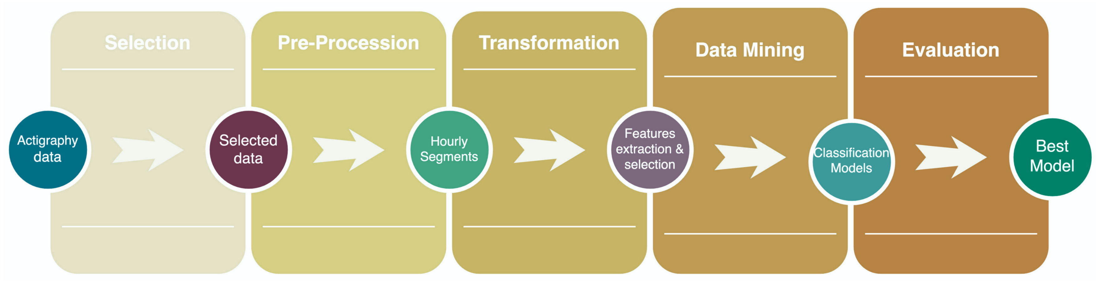
| KDD Process | |
|---|---|
| Pre-KDD | Precision psychiatry using ML algorithms’ principal objectives of treatment response analysis, early identification, suicide prevention, real-time monitoring, and subclassified actual mental disorders [33]. In addition, ML models avoid generic diagnoses, providing new classifications of individuals by their features [40]. |
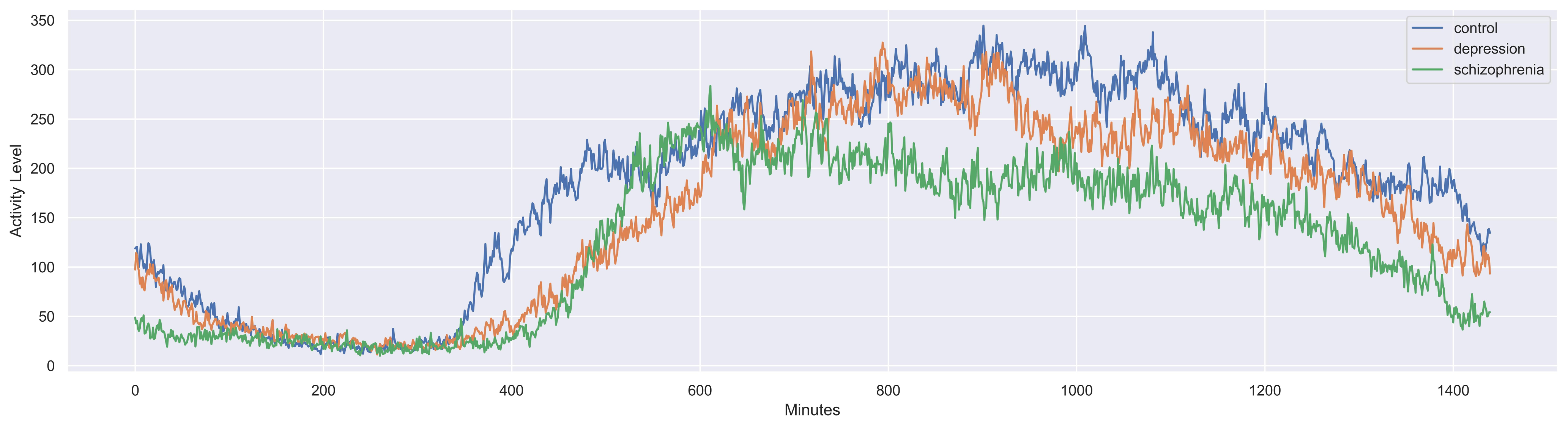
| Selection | The Depresjon and Psykose datasets contain monitor-activity counts of patients with depression and schizophrenia, respectively. |
| Preprocessing | All patients’ activity count data are concatenated into a single matrix, standardized, transposed, and grouped by hours. |
| Transformation | After hourly segmentation, data are grouped into subsets following the day stage: morning (06:00–11:59), afternoon (12:00–17:59), evening (18:00–23:59), and night (00:00–05:59). |
| Data Mining | Classification of depressive, schizophrenic, and control episodes is performed with a random forest classifier. |
| Interpretation/evaluation | Precision, recall, F1 score, MCC, and accuracy measure every model’s effectiveness to identify healthy, schizophrenic, and depressive episodes concerning the day stage. |
| Post-KDD | It is not limited to this written report. |
2.1. Selection
2.2. Preprocessing
2.3. Transformation
2.3.1. Feature Extraction
2.3.2. Feature Selection
2.4. Data Mining
- 900 trees in the forest;
- at least three samples were required to split a node;
- to be at a leaf node, the minimum required six samples;
- the maximal number of leaf nodes in a tree was 90;
- not bootstrapping the samples used the entire dataset to construct every tree.
2.5. Evaluation
3. Results
4. Discussion and Conclusions
Author Contributions
Funding
Institutional Review Board Statement
Informed Consent Statement
Data Availability Statement
Acknowledgments
Conflicts of Interest
References
- Haroz, E.; Ritchey, M.; Bass, J.; Kohrt, B.; Augustinavicius, J.; Michalopoulos, L.; Burkey, M.; Bolton, P. How is depression experienced around the world? A systematic review of qualitative literature. Soc. Sci. Med. 2017, 183, 151–162. [Google Scholar] [CrossRef] [PubMed] [Green Version]
- Friedrich, M.J. Depression is the leading cause of disability around the world. JAMA 2017, 317, 1517. [Google Scholar] [CrossRef] [PubMed]
- Ettman, C.; Abdalla, S.; Cohen, G.; Sampson, L.; Vivier, P.; Galea, S. Prevalence of depression symptoms in US adults before and during the COVID-19 pandemic. JAMA Netw. Open. 2020, 3, e2019686. [Google Scholar] [CrossRef] [PubMed]
- Aalbers, G.; McNally, R.J.; Heeren, A.; De Wit, S.; Fried, E.I. Social media and depression symptoms: A network perspective. J. Exp. Psychol. Gen. 2019, 148, 1454. [Google Scholar] [CrossRef] [PubMed] [Green Version]
- Steinberg, J.W.; Daniel, J. Depression as a major mental health problem for the behavioral health care industry. J. Health Sci. Manag. Public Health 2020, 1, 44–49. [Google Scholar]
- Charlson, F.J.; Ferrari, A.J.; Santomauro, D.F.; Diminic, S.; Stockings, E.; Scott, J.G.; McGrath, J.J.; Whiteford, H.A. Global epidemiology and burden of schizophrenia: Findings from the global burden of disease study 2016. Schizophr. Bull. 2018, 44, 1195–1203. [Google Scholar] [CrossRef]
- Moreno-Küstner, B.; Martin, C.; Pastor, L. Prevalence of psychotic disorders and its association with methodological issues. A systematic review and meta-analyses. PLoS ONE 2018, 13, e0195687. [Google Scholar] [CrossRef]
- Karagianis, J.; Novick, D.; Pecenak, J.; Haro, J.M.; Dossenbach, M.; Treuer, T.; Montgomery, W.; Walton, R.; Lowry, A. Worldwide-Schizophrenia Outpatient Health Outcomes (W-SOHO): Baseline characteristics of pan-regional observational data from more than 17,000 patients. Int. J. Clin. Pract. 2009, 63, 1578–1588. [Google Scholar] [CrossRef]
- Brisch, R.; Saniotis, A.; Wolf, R.; Bielau, H.; Bernstein, H.G.; Steiner, J.; Bogerts, B.; Braun, K.; Jankowski, Z.; Kumaratilake, J.; et al. The role of dopamine in schizophrenia from a neurobiological and evolutionary perspective: Old fashioned, but still in vogue. Front. Psychiatry 2014, 5, 47. [Google Scholar]
- Steinau, S.; Stegmayer, K.; Lang, F.U.; Jäger, M.; Strik, W.; Walther, S. Comparison of psychopathological dimensions between major depressive disorder and schizophrenia spectrum disorders focusing on language, affectivity and motor behavior. Psychiatry Res. 2017, 250, 169–176. [Google Scholar] [CrossRef]
- Sher, L.; Kahn, R.S. Suicide in schizophrenia: An educational overview. Medicina 2019, 55, 361. [Google Scholar] [CrossRef] [Green Version]
- Upthegrove, R.; Marwaha, S.; Birchwood, M. Depression and schizophrenia: Cause, consequence, or trans-diagnostic issue? Schizophr. Bull. 2017, 43, 240–244. [Google Scholar] [CrossRef] [Green Version]
- Inoue, K.; Otsuka, K.; Onishi, H.; Cho, Y.; Shiraishi, M.; Narita, K.; Kawanishi, C. Multi-institutional survey of suicide death among inpatients with schizophrenia in comparison with depression. Asian J. Psychiatry 2020, 48, 101908. [Google Scholar] [CrossRef]
- Cosgrave, J.; Wulff, K.; Gehrman, P. Sleep, circadian rhythms, and schizophrenia: Where we are and where we need to go. Curr. Opin. Psychiatry 2018, 31, 176–182. [Google Scholar] [CrossRef]
- Vahia, I.V.; Sewell, D.D. Late-life depression: A role for accelerometer technology in diagnosis and management. Am. J. Psychiatry 2016, 173, 763–768. [Google Scholar] [CrossRef] [Green Version]
- Hombali, A.; Seow, E.; Yuan, Q.; Chang, S.H.S.; Satghare, P.; Kumar, S.; Verma, S.K.; Mok, Y.M.; Chong, S.A.; Subramaniam, M. Prevalence and correlates of sleep disorder symptoms in psychiatric disorders. Psychiatry Res. 2019, 279, 116–122. [Google Scholar] [CrossRef]
- Echeburúa, E.; Salaberria, K.; Cruz-Saez, M. Contributions and limitations of DSM-5 from Clinical Psychology. Ter. Psicol. 2014, 32, 65–74. [Google Scholar] [CrossRef] [Green Version]
- Fernandes, B.S.; Williams, L.M.; Steiner, J.; Leboyer, M.; Carvalho, A.F.; Berk, M. The new field of ‘precision psychiatry’. BMC Med. 2017, 15, 1–7. [Google Scholar] [CrossRef]
- Bzdok, D.; Meyer-Lindenberg, A. Machine learning for precision psychiatry: Opportunities and challenges. Biol. Psychiatry Cogn. Neurosci. Neuroimaging 2018, 3, 223–230. [Google Scholar] [CrossRef] [Green Version]
- Corcoran, C.M.; Cecchi, G.A. Computational approaches to behavior analysis in psychiatry. Neuropsychopharmacology 2018, 43, 225. [Google Scholar] [CrossRef] [Green Version]
- Zhou, Z.; Wu, T.C.; Wang, B.; Wang, H.; Tu, X.M.; Feng, C. Machine learning methods in psychiatry: A brief introduction. Gen. Psychiatry 2020, 33, 20–22. [Google Scholar] [CrossRef] [Green Version]
- Schnack, H.G.; Nieuwenhuis, M.; van Haren, N.E.; Abramovic, L.; Scheewe, T.W.; Brouwer, R.M.; Pol, H.E.H.; Kahn, R.S. Can structural MRI aid in clinical classification? A machine learning study in two independent samples of patients with schizophrenia, bipolar disorder and healthy subjects. Neuroimage 2014, 84, 299–306. [Google Scholar] [CrossRef]
- Han, W.; Sorg, C.; Zheng, C.; Yang, Q.; Zhang, X.; Ternblom, A.; Mawuli, C.B.; Gao, L.; Luo, C.; Yao, D.; et al. Low-rank network signatures in the triple network separate schizophrenia and major depressive disorder. Neuroimage Clin. 2019, 22, 101725. [Google Scholar] [CrossRef]
- Smagula, S.F.; Chahine, L.; Metti, A.; Rangarajan, A.; Aizenstein, H.J.; Tian, Q.; Rosano, C. Regional gray matter volume links rest-activity rhythm fragmentation with past cognitive decline. Am. J. Geriatr. Psychiatry 2020, 28, 248–251. [Google Scholar] [CrossRef]
- Kluge, A.; Kirschner, M.; Hager, O.M.; Bischof, M.; Habermeyer, B.; Seifritz, E.; Walther, S.; Kaiser, S. Combining actigraphy, ecological momentary assessment and neuroimaging to study apathy in patients with schizophrenia. Schizophr. Res. 2018, 195, 176–182. [Google Scholar] [CrossRef]
- Berle, J.O.; Hauge, E.R.; Oedegaard, K.J.; Holsten, F.; Fasmer, O.B. Actigraphic registration of motor activity reveals a more structured behavioural pattern in schizophrenia than in major depression. BMC Res. Notes 2010, 3, 1–7. [Google Scholar] [CrossRef] [Green Version]
- Tazawa, Y.; Wada, M.; Mitsukura, Y.; Takamiya, A.; Kitazawa, M.; Yoshimura, M.; Mimura, M.; Kishimoto, T. Actigraphy for evaluation of mood disorders: A systematic review and meta-analysis. J. Affect. Disord. 2019, 253, 257–269. [Google Scholar] [CrossRef]
- Wee, Z.Y.; Yong, S.W.L.; Chew, Q.H.; Guan, C.; Lee, T.S.; Sim, K. Actigraphy studies and clinical and biobehavioural correlates in schizophrenia: A systematic review. J. Neural Transm. 2019, 126, 531–558. [Google Scholar] [CrossRef]
- Ransing, R.; Patil, P.; Khapri, A.; Mahindru, A. A Systematic Review of Studies Comparing Actigraphy Indices in Patients with Depression and Schizophrenia. J. Clin. Diagn. Res. 2021, 15, 1–4. [Google Scholar] [CrossRef]
- Rodríguez-Ruiz, J.G.; Galván-Tejada, C.E.; Zanella-Calzada, L.A.; Celaya-Padilla, J.M.; Galván-Tejada, J.I.; Gamboa-Rosales, H.; Luna-García, H.; Magallanes-Quintanar, R.; Soto-Murillo, M.A. Comparison of night, day and 24 h motor activity data for the classification of depressive episodes. Diagnostics 2020, 10, 162. [Google Scholar] [CrossRef] [Green Version]
- Yagoda, S.; Wolz, R.; Weiden, P.J.; Claxton, A.; Yao, B.; Du, Y. M105. Actigraphic monitoring of sleep-wake cycle in schizophrenia outpatients receiving A long-acting injectable antipsychotic: Feasibility and initial results from a prospective RCT. Schizophr. Bull. 2020, 46, S175. [Google Scholar] [CrossRef]
- Tubbs, A.S.; Fernandez, F.X.; Perlis, M.L.; Hale, L.; Branas, C.C.; Barrett, M.; Chakravorty, S.; Khader, W.; Grandner, M.A. Suicidal ideation is associated with nighttime wakefulness in a community sample. Sleep 2021, 44, zsaa128. [Google Scholar] [CrossRef] [PubMed]
- Passos, I.C.; Ballester, P.; Rabelo-da Ponte, F.D.; Kapczinski, F. Precision Psychiatry: The Future Is Now. Can. J. Psychiatry 2021, 67, 21–25. [Google Scholar] [CrossRef] [PubMed]
- Schelter, S.; Biessmann, F.; Januschowski, T.; Salinas, D.; Seufert, S.; Szarvas, G. On challenges in machine learning model management. OpenReview 2018, 41, 5–15. [Google Scholar]
- Alonso, S.G.; de la Torre-Díez, I.; Hamrioui, S.; López-Coronado, M.; Barreno, D.C.; Nozaleda, L.M.; Franco, M. Data mining algorithms and techniques in mental health: A systematic review. J. Med. Syst. 2018, 42, 1–15. [Google Scholar] [CrossRef]
- Dåderman, A.; Rosander, S. Evaluating frameworks for implementing machine learning in signal processing: A comparative study of CRISP-DM, SEMMA and KDD. Digit. Vetensk. Ark. 2018, 38, 1–43. [Google Scholar]
- Wang, Z.; Ma, Z.; An, Z.; Huang, F. A Novel Diagnosis Method of Depression Based on EEG and Convolutional Neural Network. In Proceedings of the International Conference on Frontier Computing; Springer: Singapore, 2022; pp. 91–102. [Google Scholar]
- Wanderley Espinola, C.; Gomes, J.C.; Mônica Silva Pereira, J.; dos Santos, W.P. Detection of major depressive disorder, bipolar disorder, schizophrenia and generalized anxiety disorder using vocal acoustic analysis and machine learning: An exploratory study. Res. Biomed. Eng. 2022, 1–17. [Google Scholar] [CrossRef]
- Bondugula, R.K.; Sivangi, K.B.; Udgata, S.K. Identification of Schizophrenic Individuals Using Activity Records through Visualization of Recurrent Networks. In Intelligent Systems; Springer: Berlin, Germany, 2022; pp. 653–664. [Google Scholar]
- Cearns, M.; Hahn, T.; Baune, B.T. Recommendations and future directions for supervised machine learning in psychiatry. Transl. Psychiatry 2019, 9, 1–12. [Google Scholar] [CrossRef] [Green Version]
- Jakobsen, P.; Garcia-Ceja, E.; Stabell, L.A.; Oedegaard, K.J.; Berle, J.O.; Thambawita, V.; Hicks, S.A.; Halvorsen, P.; Fasmer, O.B.; Riegler, M.A. PSYKOSE: A Motor Activity Database of Patients with Schizophrenia. In Proceedings of the 2020 IEEE 33rd International Symposium on Computer-Based Medical Systems (CBMS), Rochester, MN, USA, 28–30 July 2020; pp. 303–308. [Google Scholar]
- Garcia-Ceja, E.; Riegler, M.; Jakobsen, P.; Tørresen, J.; Nordgreen, T.; Oedegaard, K.J.; Fasmer, O.B. Depresjon: A motor activity database of depression episodes in unipolar and bipolar patients. In Proceedings of the the 9th ACM Multimedia Systems Conference, Amsterdam, The Netherlands, 12–15 June 2018; pp. 472–477. [Google Scholar] [CrossRef] [Green Version]
- Graña, A.F. Sensors of Force, Displacement and Acceleration for Biomedical Use: Physical Principles, Features and Costs. In Proceedings of the XXVI Seminario de Ingeniería Biomédica, Montevideo, Uruguay, 7 March–28 June 2017. [Google Scholar]
- Rajoub, B. Characterization of biomedical signals: Feature engineering and extraction. In Biomedical Signal Processing and Artificial Intelligence in Healthcare; Elsevier: Amsterdam, The Netherlands, 2020; pp. 29–50. [Google Scholar]
- Saha, S.S.; Rahman, S.; Rasna, M.J.; Zahid, T.B.; Islam, A.M.; Ahad, M.A.R. Feature extraction, performance analysis and system design using the du mobility dataset. IEEE Access 2018, 6, 44776–44786. [Google Scholar] [CrossRef]
- Oung, Q.W.; Basah, S.N.; Muthusamy, H.; Vijean, V.; Lee, H.; Khairunizam, W.; Bakar, S.A.; Razlan, Z.M.; Ibrahim, Z. Objective Evaluation of Freezing of Gait in Patients with Parkinson’s Disease through Machine Learning Approaches. In Proceedings of the 2018 International Conference on Computational Approach in Smart Systems Design and Applications (ICASSDA), Kuching, Malaysia, 15–17 August 2018; pp. 1–7. [Google Scholar]
- Khalid, S.; Khalil, T.; Nasreen, S. A survey of feature selection and feature extraction techniques in machine learning. In Proceedings of the 2014 Science and Information Conference, London, UK, 27–29 August 2014; pp. 372–378. [Google Scholar]
- Cai, J.; Luo, J.; Wang, S.; Yang, S. Feature selection in machine learning: A new perspective. Neurocomputing 2018, 300, 70–79. [Google Scholar] [CrossRef]
- Cho, G.; Yim, J.; Choi, Y.; Ko, J.; Lee, S.H. Review of machine learning algorithms for diagnosing mental illness. Psychiatry Investig. 2019, 16, 262. [Google Scholar] [CrossRef] [Green Version]
- Lentzas, A.; Vrakas, D. Non-intrusive human activity recognition and abnormal behavior detection on elderly people: A review. Artif. Intell. Rev. 2019, 53, 1–47. [Google Scholar] [CrossRef]
- Palop, J.J.; Mucke, L.; Roberson, E.D. Quantifying biomarkers of cognitive dysfunction and neuronal network hyperexcitability in mouse models of Alzheimer’s disease: Depletion of calcium-dependent proteins and inhibitory hippocampal remodeling. In Alzheimer’s Disease and Frontotemporal Dementia; Springer: Berlin, Germany, 2010; pp. 245–262. [Google Scholar]

| Name | Equation |
|---|---|
| Mean | |
| Sum | |
| Maximum | |
| Minimum | |
| Median | |
| Standard deviation | |
| First decile | |
| Second decile | |
| First quantile | |
| Third decile | |
| Fourth decile | |
| Second quantile | |
| Sixth decile | |
| Seventh decile | |
| Third quantile | |
| Eighth decile | |
| Ninth decile | |
| Kurtosis | |
| Mean absolute deviation | |
| Standard error of mean | |
| Skewness | |
| Variance | |
| Unique | |
| where n is the size of sample, is an item of the sample, is the fourth standardized moment, and is the third standardized moment. | |
| Day Stage | No. Features | Features |
|---|---|---|
| 00:00–05:59 | 5 | min, quantile10, quantile20, quantile25, quantile30 |
| 06:00–11:59 | 7 | min, median, quantile10, quantile20, quantile25, quantile30, quantile40 |
| 12:00–17:59 | 8 | max, min, quantile10, quantile20, quantile25, quantile30, quantile40, quantile60 |
| 18:00–23:59 | 6 | min, quantile10, quantile20, quantile25, quantile30, quantile40 |
| Day Stage | Training Instances | Testing Instances | Features |
|---|---|---|---|
| 00:00–06:00 | 6116 | 2622 | 5 |
| 06:00–12:00 | 5051 | 2165 | 6 |
| 12:00–18:00 | 4809 | 2061 | 8 |
| 18:00–00:00 | 4761 | 2041 | 7 |
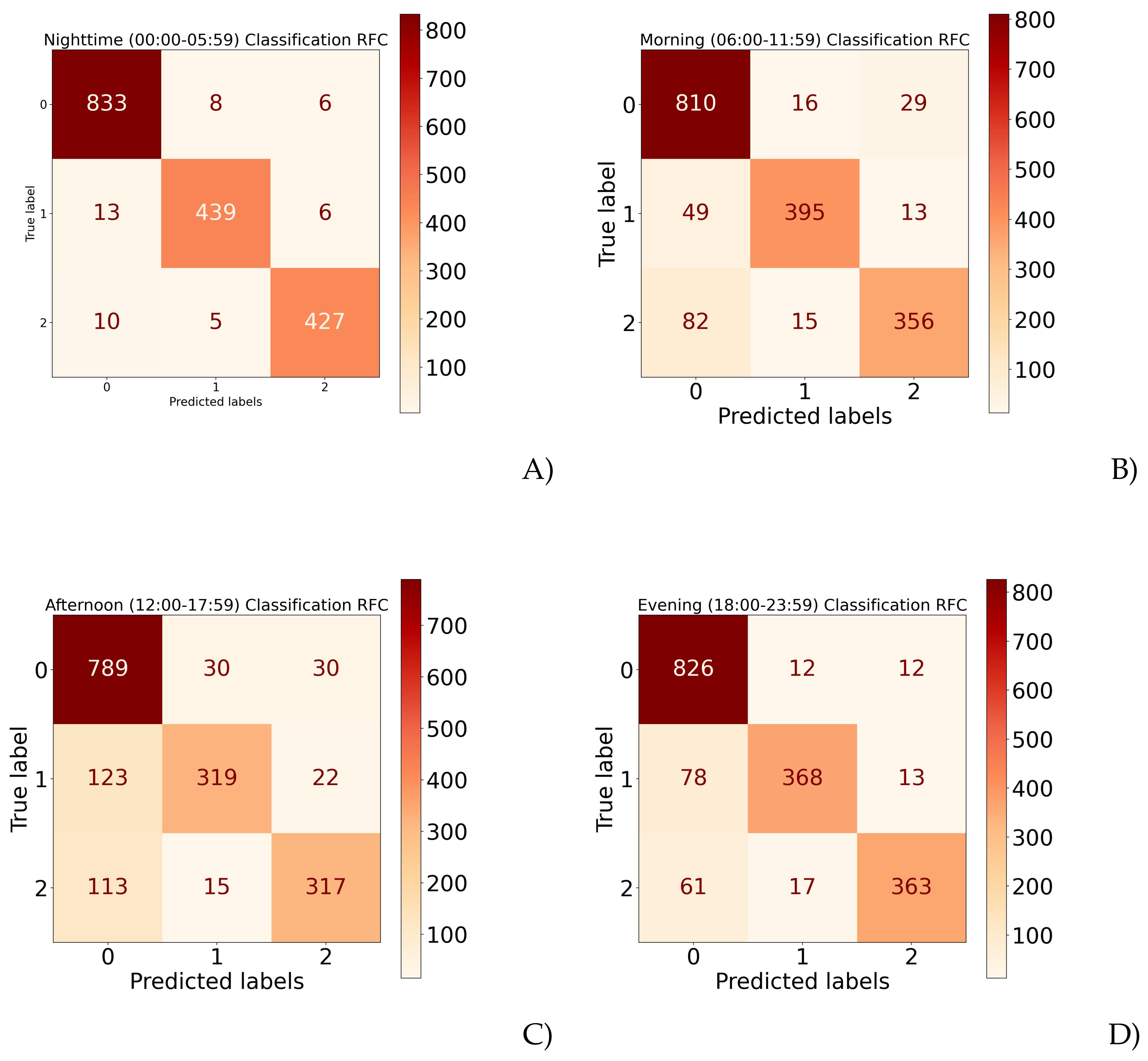
| Model | Accuracy | |
|---|---|---|
| Nighttime (00:00–05:59) | Maximum | 98.62% |
| Minimum | 97.25% | |
| Overall | 98.24% | |
| Morning (06:00–11:59) | Maximum | 88.44% |
| Minimum | 87.47% | |
| Overall | 87.97% | |
| Afternoon (12:00–17:59) | Maximum | 81.63% |
| Minimum | 80.27% | |
| Overall | 80.92% | |
| Evening (18:00–23:59) | Maximum | 91.26% |
| Minimum | 88.97% | |
| Overall | 89.84% | |
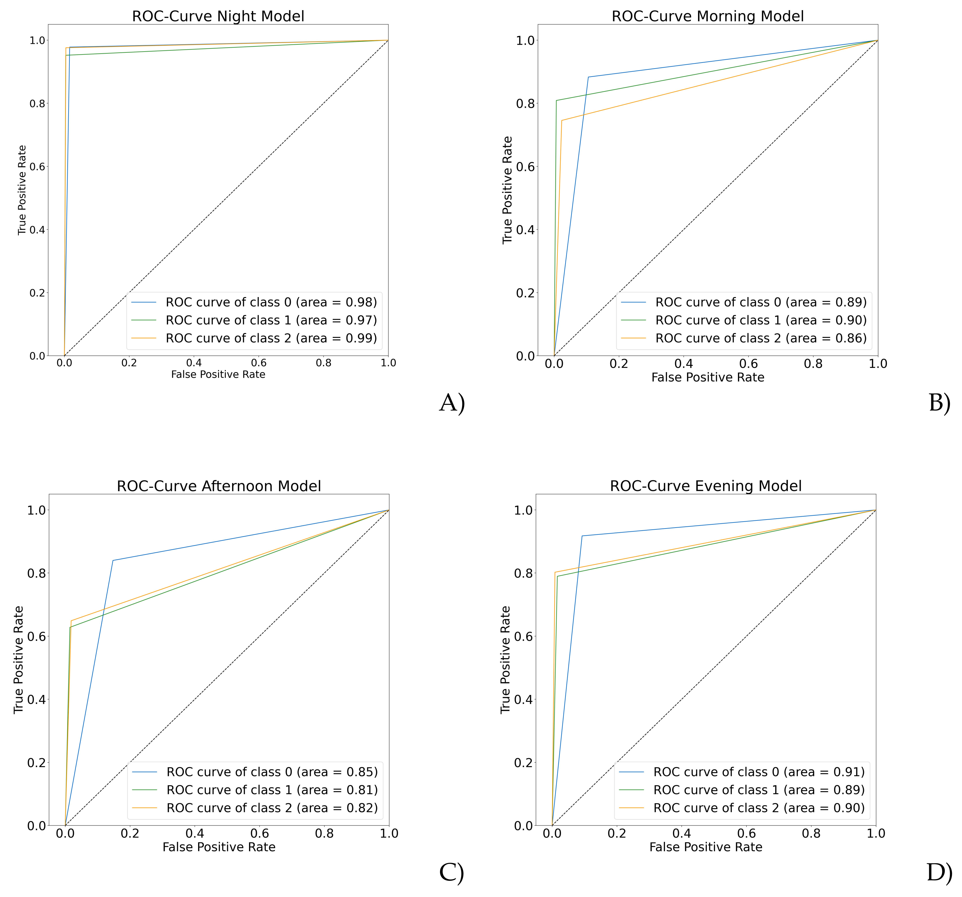
| Day Stage | Precision | Recall | F1 Score | MCC | |
|---|---|---|---|---|---|
| Night 00:00–06:00 | 0 | 0.98 | 0.99 | 0.98 | |
| 1 | 0.98 | 0.96 | 0.97 | 0.96 | |
| 2 | 0.98 | 0.98 | 0.98 | ||
| Morning 06:00–11:59 | 0 | 0.87 | 0.95 | 0.91 | |
| 1 | 0.94 | 0.85 | 0.89 | 0.81 | |
| 2 | 0.88 | 0.80 | 0.84 | ||
| Afternoon 12:00–17:59 | 0 | 0.78 | 0.91 | 0.84 | |
| 1 | 0.81 | 0.70 | 0.75 | 0.69 | |
| 2 | 0.87 | 0.72 | 0.79 | ||
| Evening 18:00–23:59 | 0 | 0.87 | 0.96 | 0.91 | |
| 1 | 0.90 | 0.84 | 0.87 | 0.82 | |
| 2 | 0.94 | 0.83 | 0.88 | ||
| Note: 0 means healthy control, 1 depressive, and 2 schizophrenic episodes. | |||||
Publisher’s Note: MDPI stays neutral with regard to jurisdictional claims in published maps and institutional affiliations. |
© 2022 by the authors. Licensee MDPI, Basel, Switzerland. This article is an open access article distributed under the terms and conditions of the Creative Commons Attribution (CC BY) license (https://creativecommons.org/licenses/by/4.0/).
Share and Cite
Rodríguez-Ruiz, J.G.; Galván-Tejada, C.E.; Luna-García, H.; Gamboa-Rosales, H.; Celaya-Padilla, J.M.; Arceo-Olague, J.G.; Galván Tejada, J.I. Classification of Depressive and Schizophrenic Episodes Using Night-Time Motor Activity Signal. Healthcare 2022, 10, 1256. https://doi.org/10.3390/healthcare10071256
Rodríguez-Ruiz JG, Galván-Tejada CE, Luna-García H, Gamboa-Rosales H, Celaya-Padilla JM, Arceo-Olague JG, Galván Tejada JI. Classification of Depressive and Schizophrenic Episodes Using Night-Time Motor Activity Signal. Healthcare. 2022; 10(7):1256. https://doi.org/10.3390/healthcare10071256
Chicago/Turabian StyleRodríguez-Ruiz, Julieta G., Carlos E. Galván-Tejada, Huizilopoztli Luna-García, Hamurabi Gamboa-Rosales, José M. Celaya-Padilla, José G. Arceo-Olague, and Jorge I. Galván Tejada. 2022. "Classification of Depressive and Schizophrenic Episodes Using Night-Time Motor Activity Signal" Healthcare 10, no. 7: 1256. https://doi.org/10.3390/healthcare10071256
APA StyleRodríguez-Ruiz, J. G., Galván-Tejada, C. E., Luna-García, H., Gamboa-Rosales, H., Celaya-Padilla, J. M., Arceo-Olague, J. G., & Galván Tejada, J. I. (2022). Classification of Depressive and Schizophrenic Episodes Using Night-Time Motor Activity Signal. Healthcare, 10(7), 1256. https://doi.org/10.3390/healthcare10071256