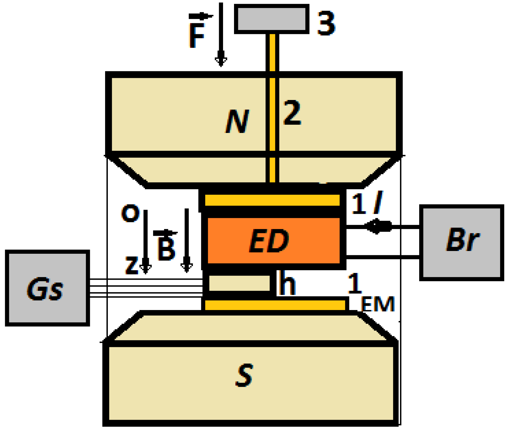
For each electrical device, ED, fixed between the N and S poles of the electromagnet, EM, the intensity of the electric current, I, was measured at the voltage generated by the internal source of Br.
3.2. Studying the Electrical Conductivity of Ms in the Presence of a Magnetic Field
Between the N and S poles of the electromagnet in
Figure 7, the devices
were inserted one by one. The voltage value at the terminals of the devices
was maintained at the value
. At Δ
t = 60 s time intervals, after fixing the
B values of the magnetic flux density, the values
of the electric current intensity were measured. As expected, the value of the intensity of the electric current through the device
indicates that there is no influence from the magnetic field. Instead, the dependence of the electric current intensity on the
B values of the magnetic flux density (increased in steps of 25 mT, up to a maximum of 275 mT) for the devices
are represented in
Figure 8.
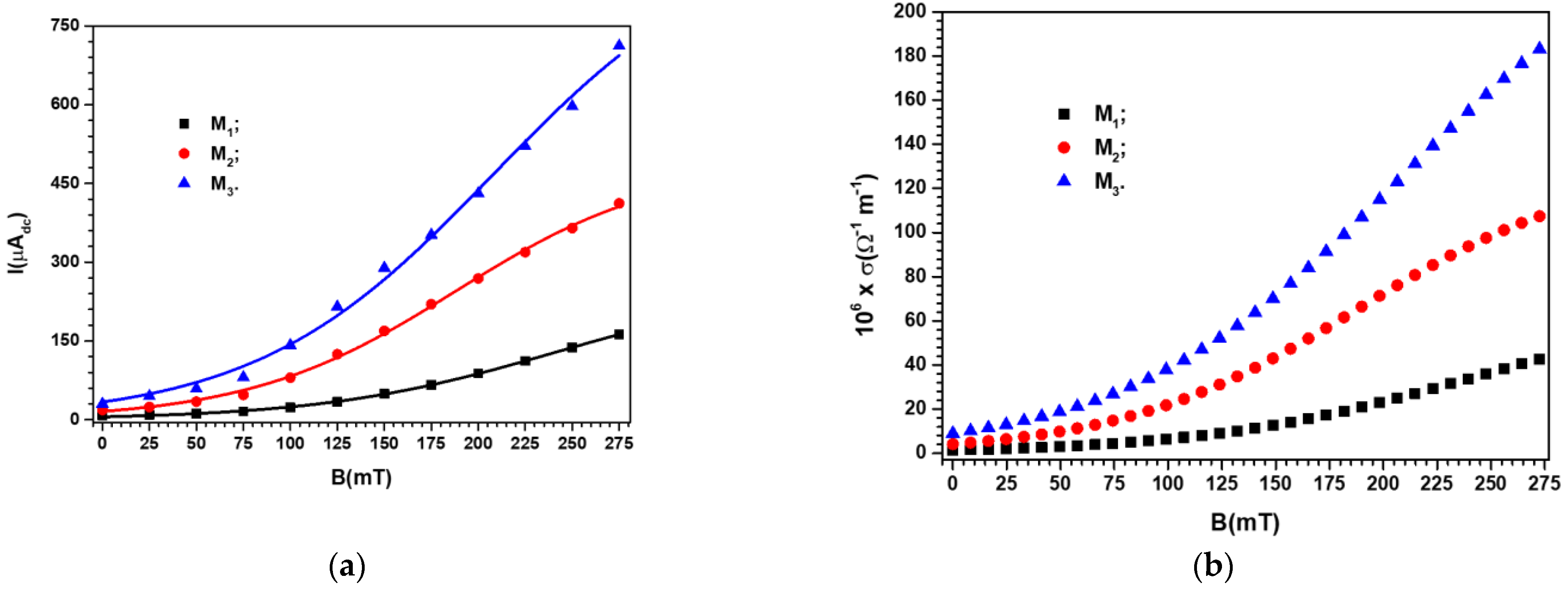
It can be seen from
Figure 8 that the electric current intensity values through the devices
were strongly influenced by the existence and concentration of metal microparticles in the body of the membranes
. For the same membrane with metal microparticles, the electric current intensity values were sensitively influenced by the B values of the magnetic flux density. Thus, when the magnetic flux density increased from
B = 25 to 275 mT, the increase in the value
I of the electric current intensity was ~30 times for membrane
, ~25 times for membrane
and ~20 times for membrane
. In the case of membranes with mixtures of carbonyl iron and silver microparticles, the decrease in the rate of the
I value of the electric current intensity is due to the decrease in the value of the volume fraction
, which is ~10% in the
membrane and ~18% in the
membrane, as can be seen from
Table 3.
For the description of the mechanisms that led to the results in
Figure 8, we considered that in the devices
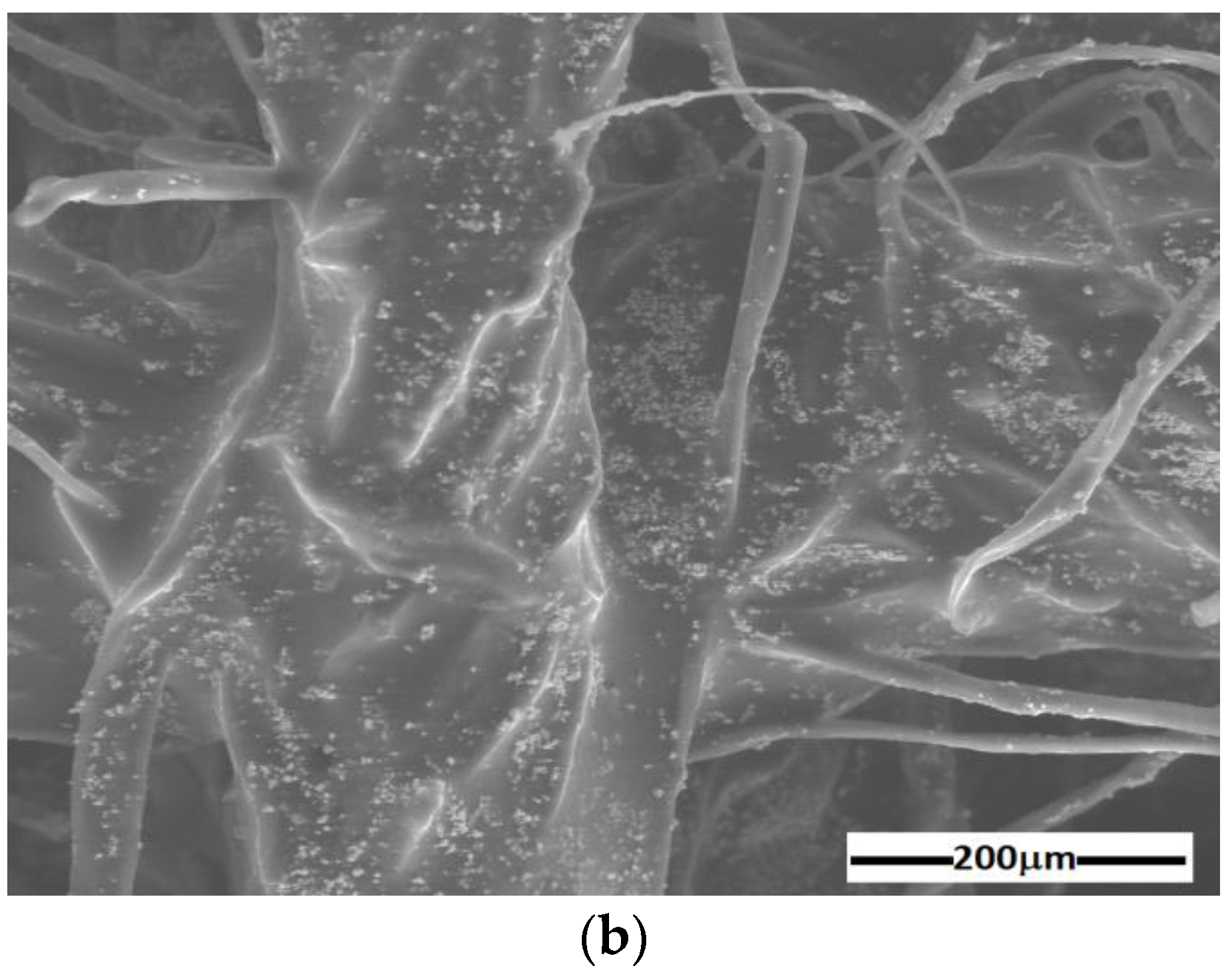
, the CI microparticles are one-dimensional and uniformly distributed in the cotton fibers impregnated with bee honey. When the magnetic field is applied (moment
t = 0 s), the CI microparticles transform, in a few moments, into magnetic dipoles. The magnetic dipoles form identical columns, equidistant and uniformly distributed in volume, in the direction of the magnetic field which is perpendicular to the surface of the membranes
[
25]. Based on the model in [
25], it is demonstrated that the magnetic force induced by the magnetic field in the volume of the membranes
can be calculated as
where
is the volume fraction of the magnetic dipoles, identically equal to the volume fraction of the carbonyl iron microparticles from
Table 3;
L,
l, and
are the length, width, and thickness of the membranes
at the moment of applying the magnetic field (
t = 0 s); and
is the magnetic permeability of the vacuum.
If, at the time t = 0, the thickness of the membranes is , then at a time t ≫ 0 after application of the magnetic field, the thickness of the membranes under the action of becomes .
It is known [
25,
26] that, in magnetorheological elastomers located in a magnetic field, there are interactions between the magnetic dipoles and between the magnetic dipoles and the respective silicone rubber that keeps them coupled. The result of the intensity of these interactions represents the resistance force opposed by the magnetorheological elastomer to the magnetic force.
Adopting this model for the membranes , which are considered continuous and deformable bodies, the force opposing the magnetic force, , is the resistance force . It acts in the same direction but opposite to the magnetic force.
The value of the force
is calculated using the following equation [
26,
27]:
where
is the magneto-deformation coupling constant of the membranes
,
is the thickness of Ms at the moment
t ≫ 0 after the application of
B, and
is the thickness of the same Ms but at the moment
t = 0 of magnetic field application.
At the moment
t = Δ
t between the forces
and
, a balance is achieved which is mathematically expressed by the equality
(with
i = 1,2, and 3). In this equality, we insert Equations (4) and (5) to obtain:
where the notation is as outlined above.
It can be seen from Equation (6) that when the magnetic field is applied, the values of the thicknesses decrease significantly with the increase in the magnetic field strength. Additionally, is dependent on the volume fraction values of CI microparticles contained in the honey impregnated in cotton microfibers, .
Considering the devices
located in the magnetic field as linear resistors, we can calculate their electrical resistance using the following equation [
26,
27,
28]:
where
is the electric voltage,
is the electric current intensity through the resistors
at the moment
t ≫ 0 after the application of
B,
is the thickness of Ms at moment
t ≫ 0 after the application of
B,
is the thickness of the same Ms but at the moment (
t = 0) of magnetic field application, and
is the conductivity of Ms, from
Table 3.
From Equations (6) and (7), we can obtain the formula for calculating the electrical resistance of devices
subjected to a magnetic field as
where
is the electrical resistance of devices
in the absence of the magnetic field given by
where the notation is as outlined above.
If a continuous and constant voltage
U is applied to the terminals of
, then an electric current passes through the resistor
with the intensity given by
where the notation is as outlined above.
We note that Equation (10) qualitatively describes the results obtained in
Figure 8a. This statement must be understood in the sense that, in the absence of the magnetic field, the values
for the constant values of the electric voltage are determined by the composition of the membranes
(see
Table 3). On the other hand, from (10), it can be observed that for the case of devices
located in a magnetic field, the values of
are strongly influenced by the B values of the magnetic field density, as we experimentally obtained in
Figure 8a.
The magneto-deformation coupling constant of the membranes
,
, extracted from Relation (10), will be
where the notation is as outlined above.
When
and the values of
from
Table 3 are inserted into Equation (11), we have
where the notation is as outlined above.
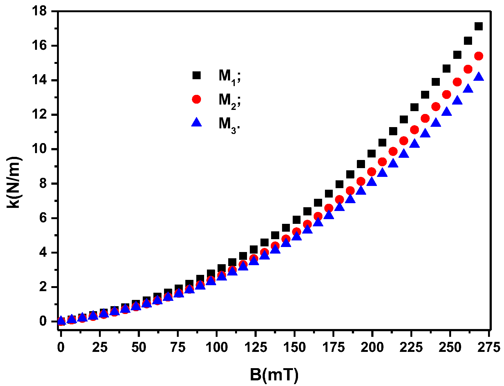
If, in the group of Relation (12), we introduce the
from
Figure 8a, we obtain the
, as shown in
Figure 9.
It can be seen from
Figure 9 that the quantities
appear when a magnetic field is applied. Their value depends on the surface area of the membranes and on the volume fractions of the magnetic dipoles,
. On the other hand, for the same membrane geometry and the same values of
, the values of
depend significantly on the density of the magnetic flux,
B. In addition, from
Figure 9, it can be seen that by adding silver microparticles, such as in the case of membranes
and
, and reducing the volume fraction of microparticles CI (see
Table 3), the value of
k decreases relative to that of membrane
for the same values of
B. This result suggests that we can consider the columns of dipoles as chains arranged in an orderly manner in the volume of the membranes
. The stiffness of the chains is dependent on the volume fraction of the magnetic dipoles and the values of the magnetic flux density
B. This result suggests that we can consider the columns with chain dipoles as being arranged in an orderly manner in the volume of the membranes
, as reported in [
28] for magnetorheological elastomers.
The decrease in the value of the volume fraction of the magnetic dipoles (see
Table 3) denotes the reduction in the number of chains and, consequently, the reduction in the value of
k for the membranes
and
compared with that of membrane
for the same value of
B, as can be seen from
Figure 9. If we introduce
from
Figure 9 into Equation (10), we obtain the polynomial fits in
Figure 8a, which are a good approximation of the experimental data.
Further, we can use Equation (3), adapted for the case of membranes
placed in a magnetic field, in which we introduce the
from
Figure 8a to obtain
represented in
Figure 8b. It can be seen from
Figure 8b that the plots of function
have the same shape and dependence on the volume fractions of conductive microparticles and the magnetic flux density values as the corresponding plots of
in
Figure 8a.
From
Table 4, it can be seen that the membranes
are characterized by an intrinsic or own electrical conductivity due to their composition (see
Table 3) and an apparent electrical conductivity (
Figure 8a,b) as an effect of the induction of magneto-deformations in Ms placed in the magnetic field, as given by Equations (6) and (9). Indeed, according to Equation (6), in the membranes placed in the magnetic field, the forces
induce deformations in the direction of the Oz coordinate axis with the following components:
where
and
are the thicknesses of the membranes
in the presence and absence of the magnetic field, respectively.
If, in Equation (13), we replace
and
from the definitions (7) and (9) of the electrical resistances in the presence and absence of the magnetic field, we can obtain the components of the deformations as
We insert the
from
Figure 8a into Equation (14) to obtain
. For each value of the magnetic flux density,
B, there are corresponding components of the deformations and values of the electrical conductivity in
Figure 8b. Similar results were reported for the case of magnetorheological elastomers [
29,
30], and for hydrogels [
31]. The deformations
correspond to the electrical conductivity values from
Figure 8b, at the same value as the magnetic field density,
B. The
σ values are due to the electronic conduction achieved through the tunnel effect [
27,
32]. As reported in [
27,
32], by increasing the values of the magnetic field density,
B, the height of the electrical potential well decreases so that the electrons from lower energy levels can pass over. The effect is the increase of electrical conductivity with the increase of
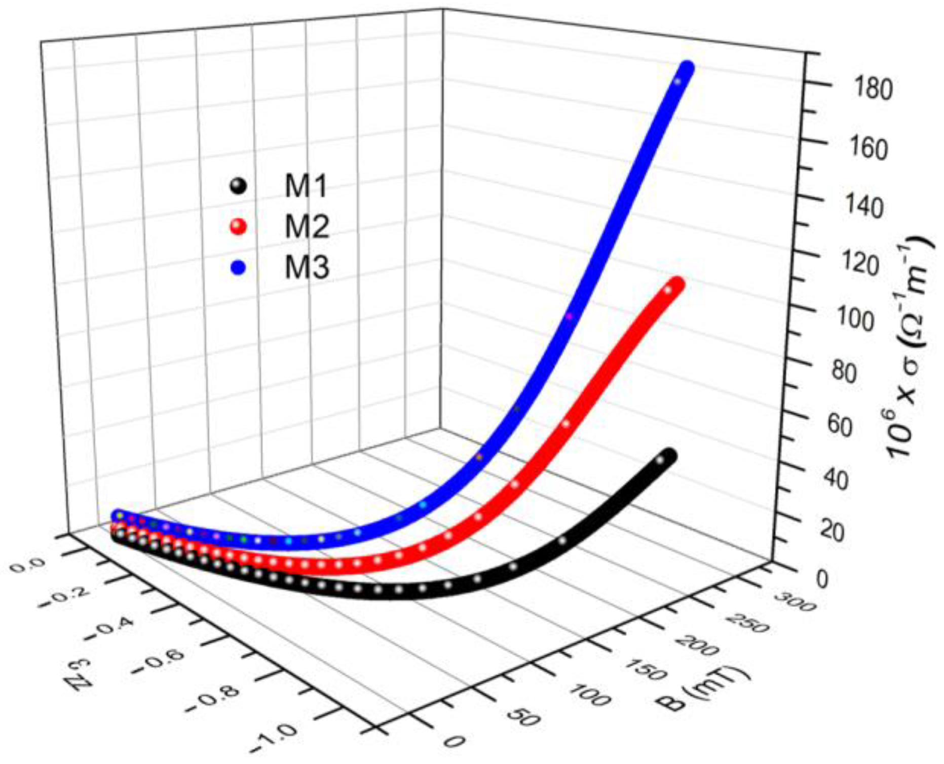
B. Through the 3D representation of the coordinate points (
B,
σ,
), we obtain
, as shown in
Figure 10.
It can be seen from
Figure 10 that for each value of the magnetic flux density,
B, deformations with the components
and apparent electrical conductivities of
are induced in the membranes
. From the same figure, we can see that the coordinate points (
B,
σ,
) depend on the composition of the membranes from
Table 3 and on the values of the magnetic flux density
B. To highlight the effect of the magnetic field on electrical conductivity, we extracted the numerical values from the 3D graph shown in
Figure 10 for two extreme values of the magnetic field, as shown in
Table 5.
It was observed that by increasing the value of the magnetic flux density, as an effect of the magneto-deformation of the membranes (see Equation (6)), the components of the deformations as well as the values of the apparent electrical conductivity increase in absolute value.


