Entropy in Tribology: in the Search for Applications

Abstract

The paper discusses the concept of entropy as applied to friction and wear. Friction and wear are classical examples of irreversible dissipative processes, and it is widely recognized that entropy generation is their important quantitative measure. On the other hand, the use of thermodynamic methods in tribology remains controversial and questions about the practical usefulness of these methods are often asked. A significant part of entropic tribological research was conducted in Russia since the 1970s. Surprisingly, many of these studies are not available in English and still not well known in the West. The paper reviews various views on the role of entropy and self-organization in tribology and it discusses modern approaches to wear and friction, which use the thermodynamic entropic method as well as the application of the mathematical concept of entropy to the dynamic friction effects (e.g., the running-in transient process, stick-slip motion, etc.) and a possible connection between the thermodynamic and information approach. The paper also discusses non-equilibrium thermodynamic approach to friction, wear, and self-healing. In general, the objective of this paper is to answer the frequently asked question “is there any practical application of the thermodynamics in the study of friction and wear?” and to show that the thermodynamic methods have potential for both fundamental study of friction and wear and for the development of new (e.g., self-lubricating) materials.

1. Introduction

The topic of this paper is the application of the concept of entropy in tribology. Tribology is defined as the science and technology of interacting surfaces in relative motion, or, in other words, the study of friction, wear and lubrication. The concept of entropy often seems difficult and confusing for non-physicists. The reason is that, unlike in the case of temperature and energy, there is no direct way of measuring entropy, so our everyday intuition does not work well when we have to deal with entropy. This is apparently the main reason why entropy, being the most important quantitative measure of disorder and dissipation, has not yet become the major tool for analyzing such dissipative processes as friction and wear.

The classical thermodynamic definition of entropy was suggested by R. Clausius in the 1860s. According to that definition, every time when the amount of heat dQ is transferred to a system at temperature T, the entropy of the system grows by

$$dS=\frac{dQ}{T}$$

(1)

Thus, when heat is transferred from a body with temperature T₁ to a body with temperature T₂, the entropy grows by dS = (1/T₂ – 1/T₁)dQ. This provides a convenient mathematical formulation for the Second Law of thermodynamics, which states that heat does not spontaneously flow from a colder body to a hotter body or, in other words, that the entropy does not decrease, just dS ≥ 0. A more formal thermodynamic definition involves the energy of a system U(S,V,N) as a function of several parameters, including entropy, volume V, and the number of particles, N. Then temperature is defined as a partial derivative of the energy of the system with respect to entropy

$$T=\frac{\partial U}{\partial S}$$

(2)

whereas the change of energy is given by

$$dU=TdS-PdV+\mu dN$$

(3)

where P is the pressure and μ is the chemical potential [1].

Note that the temperature and entropy are so-called “conjugate variables,” in a similar manner as the pressure and volume, or the chemical potential and the number of particles. For a mechanician, the most common examples of conjugate variables are the force F and distance x, defined in such a manner that the change of energy (or just the work of the force F) is given by dU = Fdx. Similarly to the force-coordinate pair F and x, the temperature, pressure, and the chemical potential are generalized forces, while entropy, volume and the number of particles are corresponding generalized coordinates. Note that the classical thermodynamic definition to entropy (as outlined in Equations 1-3) requires the internal energy U to be defined prior to the definition of entropy.

Many textbooks define entropy also as a measure of the uniformity of the distribution of energy, or a difference between the internal energy of a system and the energy available to do the useful work, known as the Helmholtz free energy A = U – TS. Every time when irreversible dissipation of energy occurs, the difference between the internal energy and the Helmholtz free energy grows, so that less energy remains available for the useful work.

A different approach to entropy was suggested by L. Boltzmann in 1877, who defined it using the concept of microstates, which correspond to a given macrostate. Microstates are arrangements of energy and matter in the system, which are distinguishable at the atomic or molecular level; however, they are indistinguishable at the macroscopic level. If Ω microstates correspond to a given macrostate, then the entropy of the macrostate is given by

S = klnΩ

(4)

where k is Boltzmann’s constant. The microstates have equal probabilities, and the system tends to evolve to a more probable macrostate, i.e., the macrostate that has a larger number of microstates [2]. The entropy definition given by Equation 4 is convenient for using entropy as a measure of disorder, since it deals with a finite (and, actually, integer) number of microstates. In the most ordered ideal state, i.e., at the absolute zero temperature, there is only one microstate and the entropy is zero. In the most disordered state of a particular system (e.g., the homogeneous mixing of two substances), the number of microstates reaches its maximum and thus the entropy is at maximum. The definition of Equation 3 can also be easily generalized for the theory of information, since the discrete microstates can be seen as bits of information required to uniquely characterize the macrostate, and thus the so-called Shannon entropy serves a measure of uncertainty in the information science.

The concept of microstate is, however, a bit obscure. It is noted, that the statistical definition of entropy given by Equation 4 implies a finite number of microstates and thus a discrete spectrum of entropy, whereas the thermodynamic definition in Equations 1-3 apparently implies a continuum spectrum of entropy and an infinite number of microstates. According to Boltzmann, the microstates should be grouped together to obtain a countable set. Two states of an atom are counted as the same state if their positions, x, and momenta, p, are within δx and δp of each other. Since the values of δx and δp can be chosen arbitrarily, the entropy is defined only up to an additive constant. However, an apparent contradiction between the continuum and discrete approach remains, so the question is often asked, whether the entropy given by Equation 1 is the same quantity as the entropy given by Equation 4? The question “what is a microstate” is not completely clarified even if we take into consideration the fact that any measurement of any parameter is conducted with a finite accuracy and, therefore, a measuring device provides a discrete rather than continuum output. Thermodynamic parameters should be independent of the resolution of our measurement devices. Some authors prefer to use the concept of “quantum states” instead of the microstates [3]; however, the classical (non-quantum) description should use classical concepts.

Fortunately, Equation 4 works independently of what is microstate. The only property of microstates that is of importance is their multiplicativity, that is, for a system consisting of two non-interacting subsystems, the total number of microstates is equal to the product of the numbers of microstates of the subsystems. This makes entropy, defined as a logarithm of the number of microstates, an additive function, that is, the entropy of a system is equal to the sum of entropies of the sub-systems. In a sense, Equation 4 serves as a definition of the microstate: the number of microstates is just an exponent of S/k. The arbitrary constant, which can be added to S, corresponds to the arbitrarily choice of δx and δp during the grouping of the microstates. The additive constant is usually chosen in such a manner that S = 0 at T = 0. In other words, there is only one microstate of any system at the absolute zero temperature when no thermal motion occurs.

While for discrete systems, microstates have a well defined meaning, for continuum systems the number of microstates is just the exponent of entropy. Therefore, another question can be asked: whether the concept of entropy provides a connecting link between the discrete and continuum systems, in other words, between energy and information? For example, the standard molar entropy (i.e., entropy per mol at the room temperature) of diamond and water is equal to 2.38 J/(K mol) and 189 J/(K mol) per mol, respectively, or, 0.3 and 22.7 per molecule. These values of entropy are calculated by integrating Equation 1 by temperature from the absolute zero to the room temperature. Does this literally mean that every atom of diamond has, on average, exp(0.3) = 1.35 microstates and every water molecule has exp(22.7) = 7.2 billion microstates? The opposite question can be asked as well. For example, the entropy of rolling a set of N dice is S = Nln6, since every die has six states. Does it mean that every time when the rolling occurs at temperature T, the amount of energy kNln(6)/T is dissipated? Indeed in order to stop a rolling die, frictional damping is needed and some dissipation always occurs; otherwise it will continue to roll forever due to the inertia. In practice, for a macroscopic die, a much larger amount of energy is dissipated than kln(6)/T. However, in the limit of a very small die, kln(6)/T is the lower limit of the energy that should be dissipated. A student of classical thermodynamics who starts to ask these questions finds quickly that an answer is found only in quantum physics, which states that most systems have a discrete spectrum of energy.

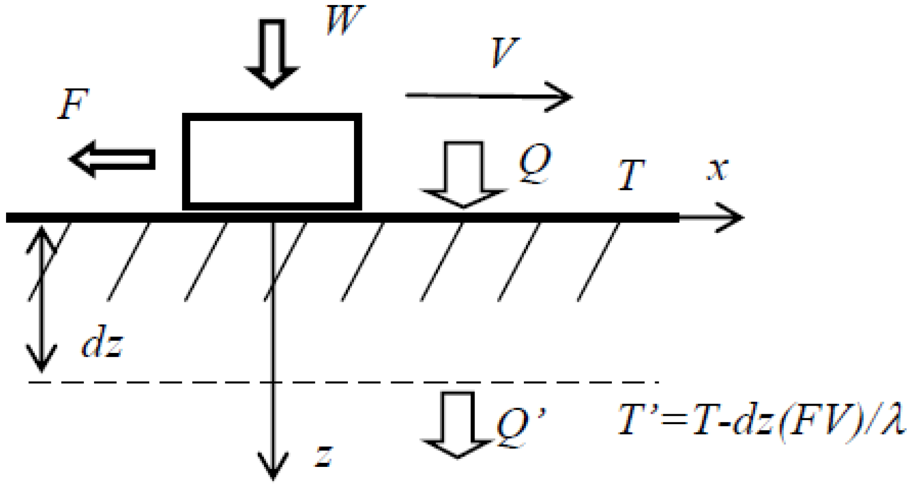
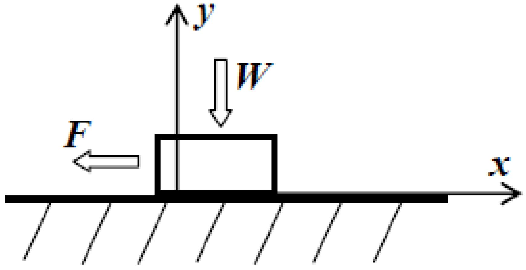
The kinetic friction is an irreversible dissipative process, during which heat is generated. For example, when the friction force F is applied to a body that passes the distance dx, the energy dQ = Fdx is dissipated into the environment, and the entropy of the environment increases for the amount of dS = F/Tdx. Furthermore, friction is a complex phenomenon which involves many diverse mechanisms, such as adhesion, elastic and plastic deformation, fracture, etc. However, in most cases it does not matter (and even not known), which particular mechanism of dissipation dominates in a particular situation, because it does not affect the macroscale properties of friction. The remarkable property of friction is its universality. It is very difficult to completely eliminate friction. Friction represents the general tendency for irreversible energy dissipation in accordance with the Second Law of thermodynamics. It is therefore reasonable to expect that the concept of entropy can capture some general properties of systems with friction, which are present irrespective of a particular mechanism of friction and thus define the phenomenon of friction.

Wear is the degradation of surface as a result of friction. While friction is manifested in the heat transfer and dissipation, wear is manifested in the mass transfer. Wear is characterized by irreversible change of surface and thus by an increase of entropy, so it is natural also to characterize wear using the concept of entropy. Despite that, the concept of entropy is rarely used in Tribology. One of the reasons is the above mentioned difficulty of the concept of entropy for the students of engineering, who prefer to use more intuitively tangible energies, temperatures, and forces in their calculations.

Historically, several attempts to use the concept of entropy in tribology were made in the Soviet Union since the 1970s. Several groups should be mentioned. First, B. Kostetsky and L. Bershadsky [4,5] at the Institute for Materials Science in Kiev investigated the formation of the so-called self-organized “secondary structures” during friction and the regime of “structural dissipative adjustment.” According to Bershadsky, friction and wear are two sides of the same phenomenon and they represent the tendency of energy and matter to achieve the most disordered state. However, the synergy of various mechanism can lead to the self-organization of the secondary structures, which are “nonstoichiometric and metastable phases,” whereas “the friction force is also a reaction on the informational (entropic) excitations, analogous to the elastic properties of a polymer, which are related mostly to the change of entropy and have the magnitude of the order of the elasticity of a gas.” [5]. Bershadsky also formulated entropic variational principles that governed friction and wear and a number of important ideas on the structural dissipative nature of friction.

Many of these ideas were influenced by the theory of self-organization developed by Ilya Prigogine (a Belgian physical chemist of the Russian origin), the winner of the 1977 Nobel Prize in Chemistry. Prigogine [6] used the ideas of Onsager’s non-equilibrium thermodynamics to describe the processes of self-organization [7]. Later, Prigogine wrote several popular books about the scientific and philosophical importance of self-organization [8,9]. At the same time, in the end of the 1970s, the concept of “Synergetics” was suggested by H. Haken [10] as an interdisciplinary science investigating the formation and self-organization of patterns and structures in open systems, which are far from thermodynamic equilibrium. The very word “synergetics” was apparently coined by the architect and philosopher R.B. Fuller (the same person, after whom the C₆₀ molecule was later called “fullerene”). The books by Prigogine and Haken were published in the USSR in Russian translations and became very popular in the 1980s among critically-minded Soviet intellectuals, since the “synergetic” studies claimed to suggest a general methodology to investigate physical, biological, information and social phenomena, which, in a sense, was (or at least, was perfected in this way by some scientists) an alternative to the official Soviet Marxist methodology. On the other hand, many more traditionally-minded theoretical physicists opposed the “synergetics,” since the synergetic studies often contained a lot of rhetoric and little practical quantitative and verifiable results [11], and even the term “pseudo-synergetics” was coined to refer to these speculative studied.

It is important to understand this historical context of the studies of self-organization during friction. According to Bershadsky [4], “tribosystems apparently constitute the most diverse objects capable for self-organization, which possess all major features of a synergetic system (strong non-linearity, parameter distribution and delay, auto-catalysis, natural regulator, feedback and target function, etc.), as well as a number of specific features, such as the energetic and materials heterogeneity, memory, learning capability, etc. This is why many unsolved tribological problems are in fact general problems of synergetics.”

The group of N. Bushe and his assistant I. Gershman at the Research Institute for the Railway Transport in Moscow is the second group that should be mentioned. To a large extent, they continued the research of the Kiev group, in particular, in the theory of “tribological compatibility” of materials, and the synergetic action of the electric current during the current collection, as well as wear resistant composite metallic coatings for heavily loaded cutting tools. Their results, which employ extensively the concept of entropy, were summarized in the monograph edited by Fox-Rabinovich and Totten [12]. In 2002, N. Bushe won the most prestigious tribology award, the Tribology Gold Medal, for his studies of tribological compatibility and other related effects.

A different approach, which also employed the concept of entropy, was suggested by Prof. Col. D. Garkunov [13] of the Air Force Academy in Russia, who claimed the discovery of the synergetic “non-deterioration effect” also called the “selective transfer.” Together with A. Polyakov, he suggested a concept of dynamically formed protective tribofilms (which they called “servovite films” or “serfing-films”). These films are formed due to a chemical reaction induced by friction and they protect against wear, leading to a dynamic equilibrium between the wear and the formation of the protective film. Garkunov’s heavily experimental research also received an international recognition when he was awarded the 2005 Tribology Gold Medal “for his achievements in tribology, especially in the fields of selective transfer.”

Among other related groups engaged in entropic studies in tribology, the scientists of Rostov and Tomsk University, Prof. K. Krawczyk of Poland, and Dr. L. Sosnovsky [14] from Gomel, Byelorussia should be mentioned. The latter suggested the concept of “tribofatika” (the coupling of wear and fatigue).

In the English-speaking world, an important entropic study of the thermodynamics of wear was conducted by M. Bryant et al. [15], who introduced a degradation function and formulated the Degradation-Entropy Generation theorem in their approach intended to study the friction and wear in complex. They note that friction and wear, which are often treated as unrelated processes, are in fact manifestations of the same dissipative physical processes occurring at sliding interfaces [16]. Their approach is based on classical Clausius’ concept of entropy.

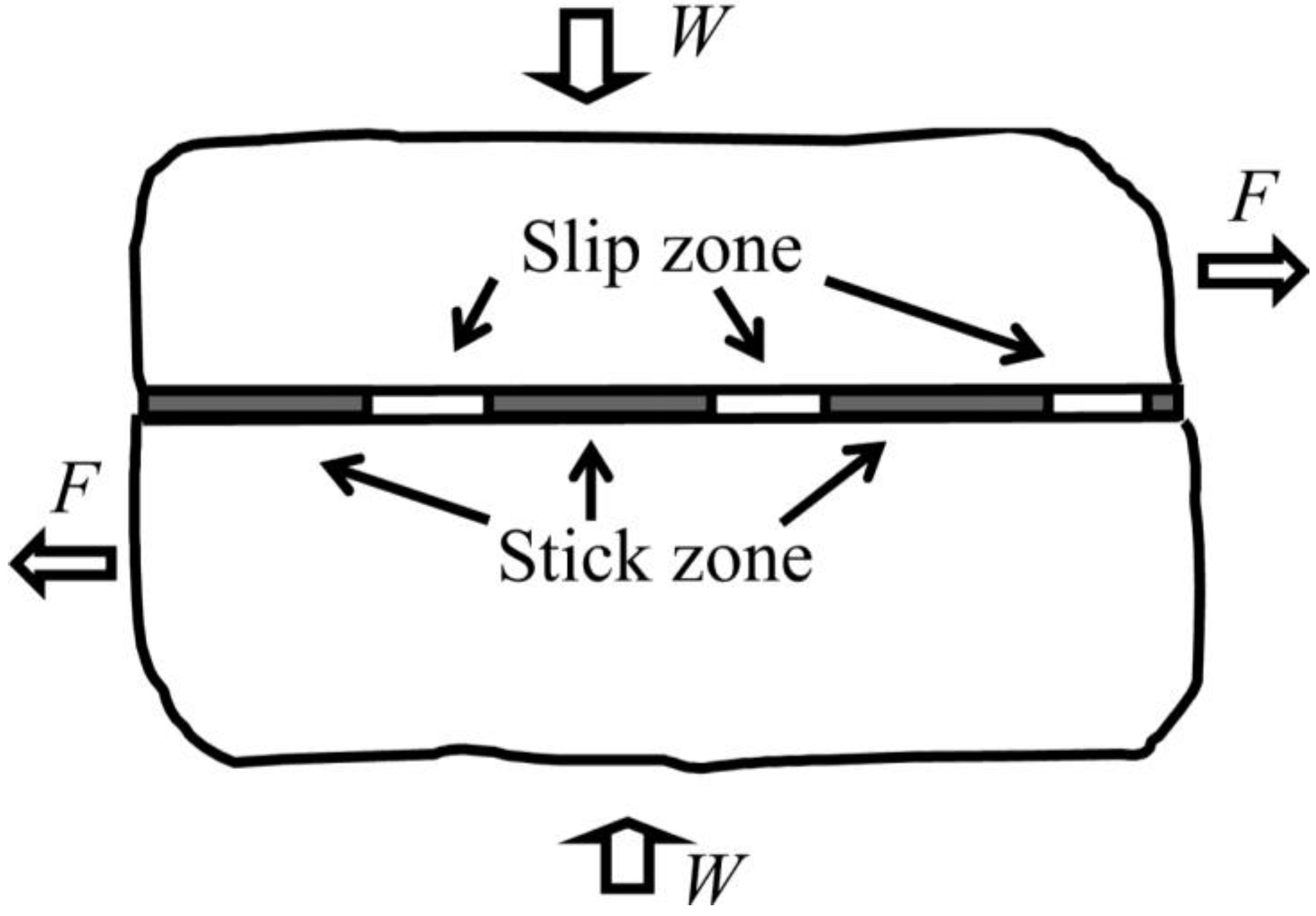
A completely different approach is related to the theory of dynamical systems. The results of friction tests can be viewed as data series characterized by certain statistical parameters, including the entropy of distributions. Since the 1980s, it has been suggested that a very specific type of self-organization, called self-organized criticality, plays a role in diverse “avalanche-like” processes, such as the stick-slip phenomenon during dry friction. The research of F. Zypman and J. Ferrante [17,18,19,20] and others deals with this topic. A different approach on the basis of the theory of dynamical systems was suggested by E. Kagan [21], and it is based on the so-called Turing systems (the diffusion-reaction systems) to describe formation of spatial and time patterns induced by friction.

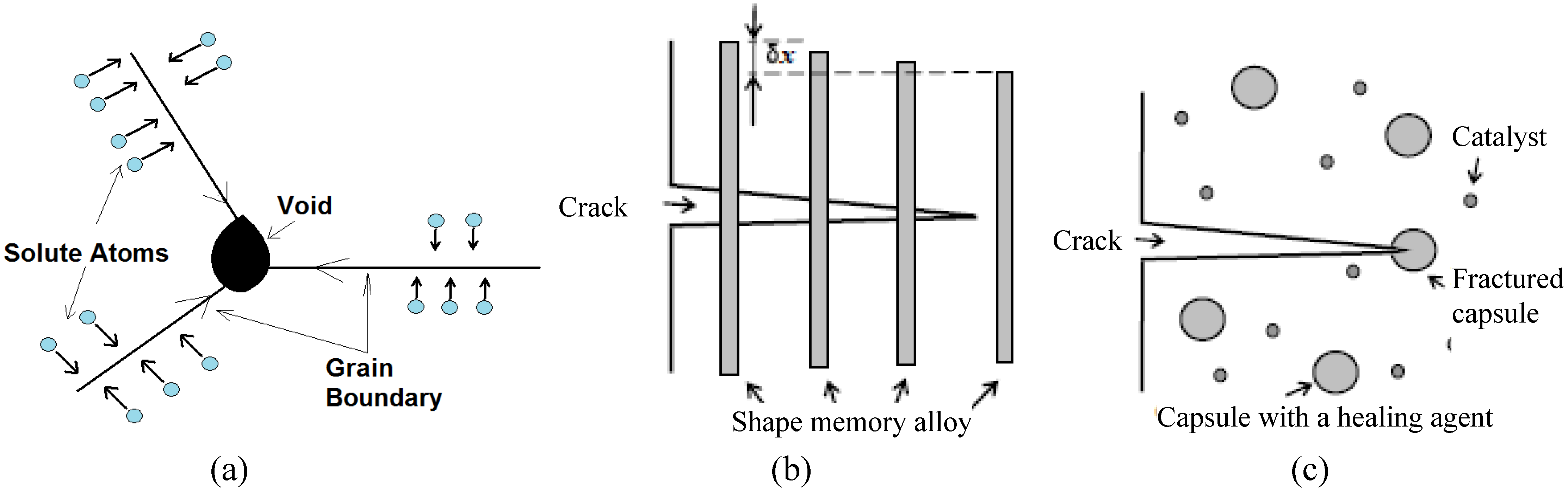
Nosonovsky and co-authors [22,23,24] suggested using the entropic methods to describe self-lubrication and surface-healing (self-healing surfaces). He noted that the orderliness at the interface can increase (and, therefore, the entropy is decreased) at the expense of the entropy either in the bulk of the body or at the microscale. He also suggested that self-organized spatial patterns (such as interface slip waves) can be studied by the methods of the theory of self-organization.

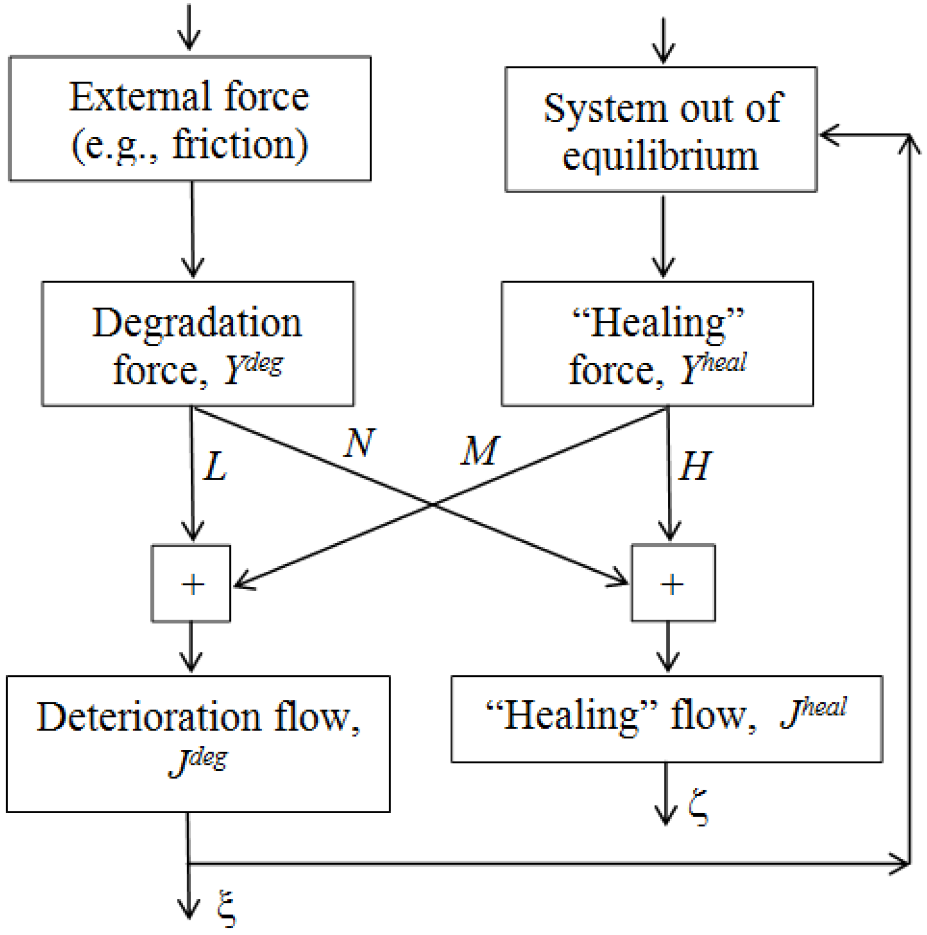
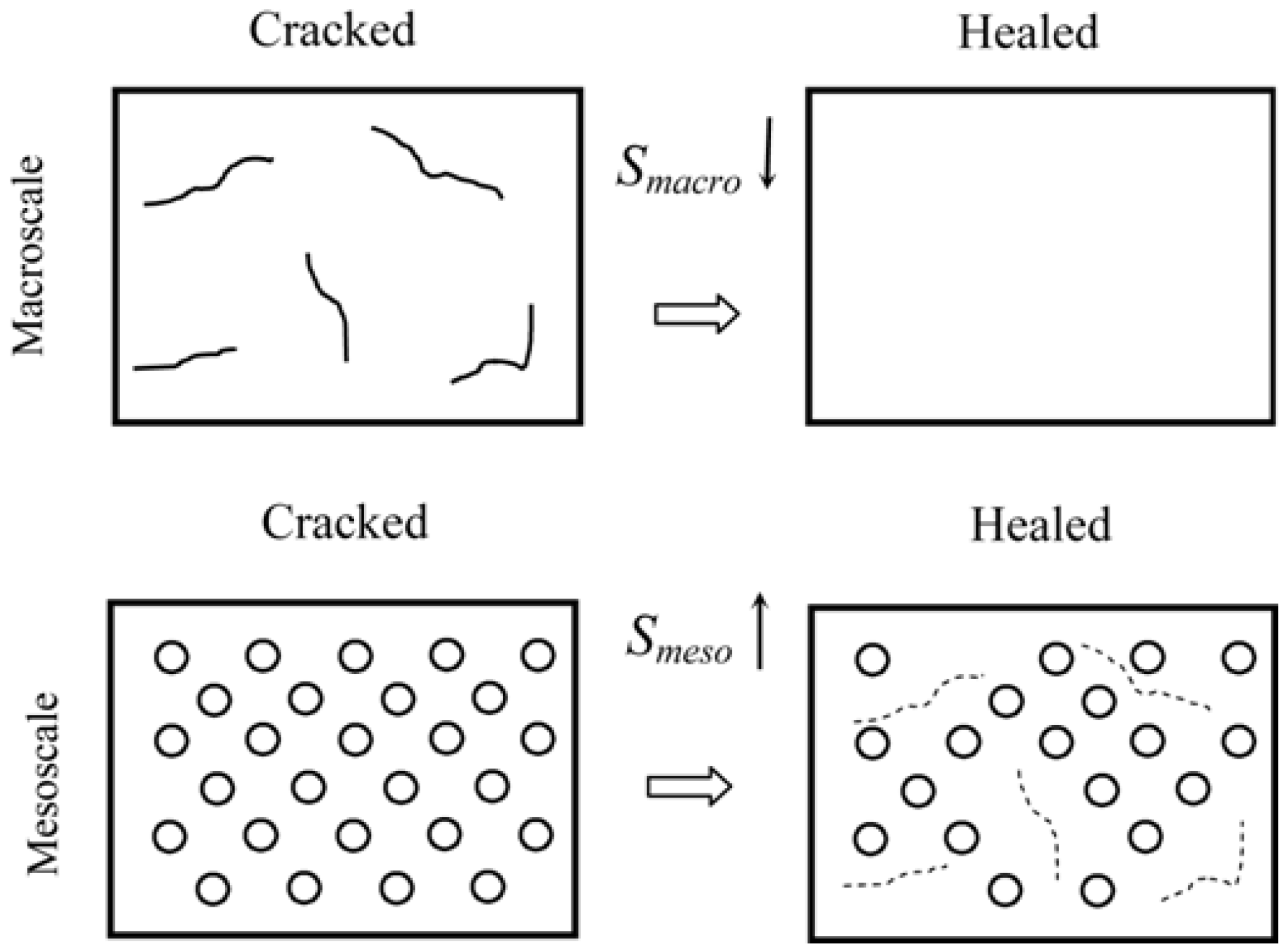
In the opinion of the author, the entropic methods are especially promising for the analysis of friction-induced self-organization, especially self-lubrication, surface-healing and self-cleaning. According to the preliminary studies, there are two key features in these processes. First, the hierarchical (multiscale) organization of the material, which allows implementing healing (as observed at the macroscale) at the expense of microscale deterioration. Second is the presence of positive and/or negative feedbacks that lead to dynamic destabilization and friction-induced vibrations. Hierarchical organization is the key feature of biological systems, which have capacity for self-organization, self-healing, and self-lubrication, so it is not surprising that hierarchy plays a central role also in artificial materials capable for self-organization. In most cases, the self-organization is induced by bringing the system out of thermodynamic equilibrium, so that the restoring force is coupled with the degradation in such a manner that healing (decreasing degradation) occurs during the return to the thermodynamic equilibrium.

The question is often asked by practical engineers and applied scientists, are there any practical benefits of using the concept of entropy in tribology? The present paper is intended to answer this question and to demonstrate practical applications, both potential and actual, of the concept of entropy, such as establishing the structure-property relationships for new materials. In this review, I will emphasize entropic approaches to friction and wear which deal with structure-property relationships, rather than speculations about entropy in friction and wear.

2. Entropy During Friction and Wear

In this section, I will discuss entropic methods of the description of friction and wear.

2.1. Friction and Dissipation

Consider a rigid body sliding upon a flat solid surface with the sliding velocity V = dx/dt (Figure 1). The normal load W is applied to the body and the friction force F = μW is generated [22]. The work of the friction force is equal to the dissipated energy, and, therefore, I will assume for now that all dissipated energy is converted into heat

$$dQ=\mu Wdx$$

(5)

The rate of entropy generation during friction is given by

$$\frac{dS}{dt}=\frac{\mu WV}{T}$$

(6)

It is noted, that friction is a non-equilibrium process. When a non-equilibrium process, which can be characterized by a parameter q (a so-called generalized coordinate), occurs, a generalized thermodynamic force X that drives the process can be introduced in such a manner that the work of the force is equal to dQ = Xdq. The flux (or flow rate) $J=\dot{q}$ is associated with the generalized coordinate. For many linear processes the flow rate is linearly proportional to Y. For sliding friction, the flow rate J = V, and the thermodynamic force X = μW/T. Note that, for the Coulombian friction, J is not proportional to Y, which is; however, the case for the viscous friction. This problem of bringing the linear friction in compliance with the linear thermodynamics will be discussed in detail in the consequent sections.

Figure 1. Heat flow away from the frictional interface.

Figure 1. Heat flow away from the frictional interface.

The net entropy growth rate for frictional sliding of rigid bodies is given by Equation 6. However, if instead of the net entropy, the entropy per surface area at the frictional interface is considered, the rate equation becomes more complicated. I consider the 1D flow of entropy near the infinite interface in the steady-state situation, and the flow is equal to entropy generation. Heat dQ is generated at the interface in accordance with Equation 5. For simplicity, I assume that all generated heat is dissipated in one of the two contacting bodies and ignore the division of heat between the two bodies. The heat is flown away from the interface in according with the heat conduction equation

$$\lambda \frac{\partial T}{\partial z}=\mu WV$$

(7)

where z is the vertical coordinate (distance from the interface), and λ is the heat conductivity. Consider a thin layer near the interface with the thickness dz. The temperature drop across the layer is dT = (μWV/λ)dz. The ratio of the heat released at the interface, dQ, to that radiated at the bottom of the layer, $d{Q}^{\prime }$, is equal to the ratio of the temperatures at the top and at the bottom of the layers

$$\frac{d{Q}^{\prime }}{dQ}=\frac{T-\mu WVdz/\lambda }{T}$$

(8)

Therefore, the energy released at the subsurface layer of depth dz is given by [22]

$$dq=\frac{dQ-d{Q}^{\prime }}{dz}=dQ\frac{\mu WV}{\lambda T}=\frac{{\left(\mu WV\right)}^2}{\lambda T}$$

(9)

Thus the entropy in the subsurface layer, dS/dt = dq/T, is given by

$$\frac{dS}{dt}=\frac{{\left(\mu WV\right)}^2}{\lambda T^2}$$

(10)

Note that S in Equation 10 is entropy per unit surface area and thus it is measured in JK⁻¹m⁻², unlike the total entropy in Equation 6, which is measured in JK⁻¹ [22,25].

The difference between Equation 6 and Equation 10 is that the latter takes into account the thermal conductivity and that in Equation 6 gives the net entropy rate, while Equation 10 gives the rate of entropy in the subsurface layer. Note the form for the thermodynamic flow is now J = μWV, and the thermodynamic force is X = μWV/(λT²).

2.2. Wear and Entropy

In the non-equilibrium (or irreversible) thermodynamics, a process that does not depend on time is called stationary, whereas a process that does not depend on the spatial coordinates is called homogeneous. A process which is both homogeneous and stationary is called equilibrium, whereas a process which is either non-stationary or inhomogeneous is called non-equilibrium. When a non-equilibrium process, which can be characterized by a parameter q (a so-called generalized coordinate), occurs, a generalized thermodynamic force Y that drives the process can be introduced in such a manner that the work of the force is equal to dQ = Ydq. The flux (or flow rate) $J=\dot{q}$ is associated with the generalized coordinate, so the entropy production rate per unit time is $\dot{S}=YJ$. For sliding friction, the flow rate is equal to the sliding velocity J = V, and the thermodynamic force is equal to the friction force Y = μW/T. Frictional sliding and wear are irreversible processes, since they are inhomogeneous and often non-stationary.

The endeavors to use thermodynamic methods to develop a general theory of wear have been taken by many researchers; however, most of these attempts had limited success due to the complexity of the equations involved and the difficulty of their solution [16,26,27]. Doelling et al. [28] experimentally correlated wear with entropy flow, dS/dt, at a wearing surface and found that wear was roughly proportional to the entropy produced for the steady sliding of copper on steel under boundary lubricated conditions. Bryant et al. [15] conducted an interesting entropic study of wear. They started from the assumption that friction and wear are manifestations of the same dissipative physical processes occurring at sliding interfaces. The production of irreversible entropy by interfacial dissipative processes is associated with both friction and wear. Friction force dissipates power and generates entropy, whereas wear irreversibly changes material’s structure, often with loss of material. Bryant [16] identified entropy production mechanisms during various dissipative processes relevant to friction and wear, which are summarized in Table 1. It is observed that the change of entropy has the general form of dS = Ydξ, that is, a thermodynamic force Y times the change of the generalized coordinate dξ.

Table 1. Entropy change during various dissipative processes (based on [16]).

Process	Entropy change
Adhesion	$dS=\frac{\gamma dA}{T}$, where γ is surface energy, A area
Plastic deformation	$dS=\frac{U_{p}dV}{T}$, where Up is the work per volume, V volume
Fracture	$dS=\frac{\left(\frac{\partial U}{\partial a}-2\gamma \right)da}{T}$, where $\frac{\partial U}{\partial a}$ is the energy release rate, a is crack length
Phase transition	$dS=\frac{dH}{T}$, where H is enthalpy
Chemical reaction	$dS=\frac{{\displaystyle \sum _{react}{\mu }_{i}d{N}_i}-{\displaystyle \sum _{products}{\mu }_{i}d{N}_i}}{T}$, where Ni are numbers of molecules and μi are chemical potentials for reactants and products.
Mixing	$\Delta S=-R{\displaystyle \sum _i^n\frac{N_i}{N}\ln \frac{N_i}{N}}$, where Ni are numbers of molecules and R is the universal gas constant
Heat transfer	$dS=\left(\frac{1}{T_1}-\frac{1}{T_2}\right)dQ$, where T1 and T2 are temperatures of the two bodies

Table 1. Entropy change during various dissipative processes (based on [16]).

Process	Entropy change
Adhesion	$dS=\frac{\gamma dA}{T}$, where γ is surface energy, A area
Plastic deformation	$dS=\frac{U_{p}dV}{T}$, where Up is the work per volume, V volume
Fracture	$dS=\frac{\left(\frac{\partial U}{\partial a}-2\gamma \right)da}{T}$, where $\frac{\partial U}{\partial a}$ is the energy release rate, a is crack length
Phase transition	$dS=\frac{dH}{T}$, where H is enthalpy
Chemical reaction	$dS=\frac{{\displaystyle \sum _{react}{\mu }_{i}d{N}_i}-{\displaystyle \sum _{products}{\mu }_{i}d{N}_i}}{T}$, where Ni are numbers of molecules and μi are chemical potentials for reactants and products.
Mixing	$\Delta S=-R{\displaystyle \sum _i^n\frac{N_i}{N}\ln \frac{N_i}{N}}$, where Ni are numbers of molecules and R is the universal gas constant
Heat transfer	$dS=\left(\frac{1}{T_1}-\frac{1}{T_2}\right)dQ$, where T1 and T2 are temperatures of the two bodies

Bryant et al. [15] also formulated the so-called “Degradation-Entropy generation theorem”, which states that for N dissipative processes, characterized by energies p_i = p_i(ζⁱ₁, ζⁱ₂,… ζⁱ_n,), where ζ_j are generalized coordinates (or “phenomenological variables”) associated with the processes, and for a degradation measure w(p₁, p₂,… p_n), which is non-negative and monotonic function of the process energies pi , the rate of degradation $\dot{w}={\displaystyle \sum _i^n{B}_i}{\dot{S}}_i$ is a linear function of the components of entropy production ${\dot{S}}_i={\displaystyle \sum _j^n{X}_i^j{J}_i^j}$ of the dissipative processes (where X and J are generalized forces and flows of the processes). Degradation components ${\dot{w}}_i={{\displaystyle \sum _j^n{Y}_i^j{J}_i^j}}_i$ proceed at rates $J_i^j$ determined by entropy production, whereas the generalized “degradation forces” $Y_i^j=B_i{Y}_i^j$are linear functions of Y_i = B_iX_i, and degradation coefficients B_i are partial derivatives of w by entropy.

For the wear process, it is natural to take wear volume as the degradation measure w. Using $\dot{w}=B\dot{S}$we obtain the wear rate

$$\frac{dw}{dt}=B\frac{\mu WV}{T}$$

(11)

For plastic contact, Equation 11 can be re-written by setting the wear coefficient k=μHB/T as

$$\frac{dw}{dt}=k\frac{WV}{H}$$

(12)

where H is hardness of a softer material in contact. For elastic contact, k = μE^*(σ/β^*)B/T yields

$$\frac{dw}{dt}=k\frac{WV}{E^{*}\left(\sigma /{\beta }^{*}\right)}$$

(13)

where E^* is the effective elastic modulus, σ is the standard deviation of rough profile height, and β^* is the correlation length of profile roughness (in a sense, σ is the height, and β^* is the length of a typical asperity). Equation 13 is widely used as the Archard equation for adhesive wear [22].

The non-trivial part of this derivation is that the wear volume per unit time is linearly proportional to the friction force for a given sliding process. This implies that (i) a constant value of energy dissipated by friction is consumed for wear debris generation and (ii) a constant amount of energy is consumed, in average per wear particle volume. Wear and friction are essentially two sides of the same dissipative process, as the energy consumed for creating wear particles is related to the work of friction. The model, however, cannot predict actual values of the wear coefficients, and its advantage is in providing theoretical foundation of the empirical laws of wear.

A different approach was suggested by Berkovich and Gromakovsky [29], who pointed out that thermodynamically wear is an irreversible mass transfer process dependent upon the local gradients of chemical potentials. The balance of energy in a tribosystem is given by

$$\mathsf{\rho }\text{TdS}=\mathsf{\rho }\text{dU}-{\mathsf{\sigma }}_{\mathrm{ik}}·\text{d}\overline{{\mathsf{\epsilon }}_{\mathrm{ik}}}-{\mathrm{N}}_{\mathrm{i}}\text{d}{\mathsf{\mu }}_{\mathrm{i}}$$

(14)

where ρ is the density, σ_ik and ε_ik are the stress and strain tensors, N_i and μ_i are the number of particles and the chemical potential of the fraction i. The mass transfer in a frictional system depends upon the heat flow, dissipation, and chemical potentials of components in the system.

Figure 2. Hidden energy density vs. the number of cycles [29].

Figure 2. Hidden energy density vs. the number of cycles [29].

According to the model by Fedorov (as presented in [29]), the probability of deterioration is proportional to the exponent of the entropy flow and relaxation time τ, which characterizes the process of restoring the thermodynamic equilibrium

$$\omega \propto \exp \left(\frac{\dot{S}\tau }{k}\right)$$

(15)

where ω is the density of defects or their “hidden energy.” The hidden energy of degradation is created by the fluctuation of thermal energy in the mechanical stress field. When the hidden energy reaches its critical density, the destruction occurs. The entropy rate in Equation 15 depends on the under the applied stress, σ. The “hidden energy density” as a function of time for steel is shown in Figure 2 for the values of stress σ = (25.3, 24.8, 23.9, 23.1, 22.5) kg/mm² and it shows an agreement with the experimental values on the deterioration as a function of the numner of cycles for various loadings [29].

It is of interest also to mention the model, suggested by Bershadsky [4,5], who also believed that friction and wear are inter-related processes that represent the trend to deteriorate for energy and matter, respectively. According to his concept of the “structural adjustment”, during the structural adjustment all types of interactions (adhesion, deformation, material transfer) are localized at the surface, which minimizes the absorbed energy ΔE in the work of friction A = ΔE+Q. As a result, the ratio of ΔE/A is minimized over the volume, so that the variational principle holds

$$\delta {\displaystyle \underset{V}{\int }\frac{\Delta E(V)}{A}dV}=0$$

(16)

According to this principle, most work is converted into heat. Dissipative ability of the material, along with its hardness, defines the wear resistance.

To summarize, the thermodynamic theories of wear provide foundation for the empirical wear laws (such as the Archard law) and suggest the principles to calculate the parameters of these laws (such as the wear coefficient).

3. Entropic Methods of Study of Self-organized Tribological Systems

While the net entropy grows in most systems in accordance with the Second law of thermodynamics, some thermodynamic systems may lead to an increasing orderliness and self-organization [6]. These are thermodynamically open systems that operate far from thermodynamic equilibrium and can exchange energy, matter, and entropy with the environment. Many of these self-organizing systems (such as the Bénard cells in boiling liquid and oscillating chemical reactions) were known a long time ago; however, the universality and generality of the processes involved in these systems was understood only with the works by Prigogine and Haken [6,7,8,9,10]. It is believed that this ability for self-organization of physical systems led to the formation of complex hierarchical chemical and biological systems.

The flow of heat, entropy, and material away from the interface during the dry friction and wear can lead to self-organization when so-called “secondary structures” form. The secondary structures are either patterns that form at the interface (e.g., stick and slip zones) or those formed as a result of mutual adjustment of the bodies in contact. The entropy production rate reaches its minimum in the self-organized state. Therefore, the self-organization is usually beneficial for the tribolological system, as it leads to the reduction of friction and wear [22].

3.1. Self-organization in Tribology

The idea that friction and wear can lead not only to deterioration, but, in some cases, to self-organization was at first suggested and investigated in the 1970-1980s. As I have already discussed in the introduction, this was under the clear influence of the “Synergetics” and philosophical ideas of Haken and Prigogine. The earlier work on self-organization is characterized by qualitative, rather than quantitative analysis of self-organization mechanisms. For example, it is noted in many of these publications that typical tribosystems possess the qualities which, according to Prigogine, are required (but not sufficient) for the self-organization, for example, that the system should be thermodynamically open, non-linear, and it should operate far from the equilibrium.

Bershadsky [4] suggested a classification of various friction-induced self-organization effects. In search of self-organization during friction he investigates quite a diverse range of processes and phenomena–auto-hydrodynamic effects, the evolution of microtopography, the formation of chemical and convective patterns, the oscillation of various parameters measured experimentally during friction. Some of these phenomena had well-investigated principles and mechanisms, while other were studied in a phenomenological manner, so it was not possible to approach them all in uniform manner. He, therefore, suggested that the state and evolution of a self-organized tribosystem might be described using different methods, including the equations of motion, statistical description, measurement of a certain parameter, etc. Depending on the method of description, different features of self-organization (“synergism”) were observed, but in most situations a self-regulated parameter existed and governing principle or target function could be identified. Table 2 summarizes the features of “synergism” in various tribological phenomena and corresponding governing principles and by target function, based on Bershadsky [4].

Table 2. Self-organization effects in tribosystems.

Effect	Description of the state or evolution	Features of synergism	Self-regulated parameter	Target function and/or governing principle
Auto-hydrodynamic effects (wedges, gaps, canyons)	Equations of motion, competing processes for entropy and negentropy production	Bifurcation; self-excited vibrations and waves; feedback and target functions	Gap thickness, temperature, and microtopography distributions	Minimum friction
Self-reproducing micro-topography, waviness	Equations of motion or kinetics	Bifurcations; self-excited vibrations and waves	Rough surface microtopography	Minimum energy dissipation; pressure or heat flow distribution
Steady state microtopography of worn surfaces (“natural wear shape”)	Competing processes for entropy and negentropy (information) production	Feedback and target function	Shape of the profile	Minimum energy dissipation
Self-excited vibrations of wear, electric resistance, stresses, etc.	Measurements of a parameter of the system (friction force, electrical resistance, wear rate, etc)	Instabilities and self-excited oscillations of the measured parameter	Corresponding parameter	Minimum entropy production
Spatial or periodic chemical pattern	Molecular, atomic, or dislocation structure	Large-scale ordered structures	Secondary heterogeneity at the surface	Dissipative principles
Periodic or concentric structures, such as Bénard cells	Molecular, atomic, or dislocation structure; Entropy is measured	Large-scale order structures; a sudden decrease in entropy production	-	Minimum entropy production
Decrease in macrofluctuation of temperature, particle size and other parameters	Order-parameter dependent on generalized coordinate, Measurements of a parameter of the system	Microfluctuations; phase transitions; instabilities and self-excited vibrations of the measured parameter	-	Sub-minimal friction

Table 2. Self-organization effects in tribosystems.

Effect	Description of the state or evolution	Features of synergism	Self-regulated parameter	Target function and/or governing principle
Auto-hydrodynamic effects (wedges, gaps, canyons)	Equations of motion, competing processes for entropy and negentropy production	Bifurcation; self-excited vibrations and waves; feedback and target functions	Gap thickness, temperature, and microtopography distributions	Minimum friction
Self-reproducing micro-topography, waviness	Equations of motion or kinetics	Bifurcations; self-excited vibrations and waves	Rough surface microtopography	Minimum energy dissipation; pressure or heat flow distribution
Steady state microtopography of worn surfaces (“natural wear shape”)	Competing processes for entropy and negentropy (information) production	Feedback and target function	Shape of the profile	Minimum energy dissipation
Self-excited vibrations of wear, electric resistance, stresses, etc.	Measurements of a parameter of the system (friction force, electrical resistance, wear rate, etc)	Instabilities and self-excited oscillations of the measured parameter	Corresponding parameter	Minimum entropy production
Spatial or periodic chemical pattern	Molecular, atomic, or dislocation structure	Large-scale ordered structures	Secondary heterogeneity at the surface	Dissipative principles
Periodic or concentric structures, such as Bénard cells	Molecular, atomic, or dislocation structure; Entropy is measured	Large-scale order structures; a sudden decrease in entropy production	-	Minimum entropy production
Decrease in macrofluctuation of temperature, particle size and other parameters	Order-parameter dependent on generalized coordinate, Measurements of a parameter of the system	Microfluctuations; phase transitions; instabilities and self-excited vibrations of the measured parameter	-	Sub-minimal friction

Nosonovsky and co-workers [22,23,24,30] suggested entropic criteria for friction-induced self-organization on the basis of the multiscale structure of the material (when self-organization at the macroscale occurs at the expense of the deterioration at the microscale) and coupling of the healing and degradation thermodynamic forces. Table 3 summarizes his interpretation of various tribological phenomena, which can be viewed as self-organization. In addition, self-organization is often a consequence of coupling of friction and wear with other processes, which creates a feedback in the tribosystem.

Table 3. Self-organization effects in tribosystems [30]

Effect	Mechanism/ driving force	Condition to initiate	Final configuration
Stationary microtopography distribution after running in	Feedback due to coupling of friction and wear	Wear affects microtopography until it reaches the stationary value	Minimum friction and wear at the stationary microtopography
In situ tribofilm formation	Chemical reaction leads to the film growth	Wear decreases with increasing film thickness	Minimum friction and wear at the stationary film thickness
Slip waves	Dynamic instability	Unstable sliding	Reduced friction
Self-lubrication	Embedded self-lubrication mechanism	Thermodynamic criteria	Reduced friction and wear
Surface-healing	Embedded self-healing mechanism	Proper coupling of degradation and healing	Reduced wear

Table 3. Self-organization effects in tribosystems [30]

Effect	Mechanism/ driving force	Condition to initiate	Final configuration
Stationary microtopography distribution after running in	Feedback due to coupling of friction and wear	Wear affects microtopography until it reaches the stationary value	Minimum friction and wear at the stationary microtopography
In situ tribofilm formation	Chemical reaction leads to the film growth	Wear decreases with increasing film thickness	Minimum friction and wear at the stationary film thickness
Slip waves	Dynamic instability	Unstable sliding	Reduced friction
Self-lubrication	Embedded self-lubrication mechanism	Thermodynamic criteria	Reduced friction and wear
Surface-healing	Embedded self-healing mechanism	Proper coupling of degradation and healing	Reduced wear

In addition, self-organization is often a consequence of coupling of friction and wear with other processes, which create a feedback in the tribosystem. These “other processes’ may include radiation, electricity, ultrasound, electric field etc. Following Haken and Prigogine, Bershadsky considered self-organization as a general property of matter, which is complimentary to wear and degradation. These ideas, while interesting from the philosophical point of view, caused the criticism of the synergetics as not being a sufficiently “scientific” field in terms of quantitative analysis. It took several decades until the investigation of spatial and temporal pattern formation during friction found a foundation in the thermodynamics and the theory of dynamical systems.

3.2. Thermally Activated Self-organization

In the preceding sections, Equations 6 and 10 were presented, which provide the total entropy rates and surface entropy rate during friction. In this section, its application to the tribosystems will be discussed. Frictional sliding and wear are irreversible processes, since they are inhomogeneous and often non-stationary. The transition from the steady state (stationary) sliding regime to the regime with self-organized structures occurs through the destabilization of the steady state regime. At the steady state, the rate of entropy production is at minimum. The stability condition for the thermodynamic system is given in the variational form by

$$\frac{1}{2}{\delta }^2\dot{S}={\displaystyle \sum _k\delta X_k\delta J_k}\ge 0$$

(17)

where ${\delta }^2\dot{S}$ is the second variation of entropy production rate [22] and k is the number of the generalized forces and flows. Equation 17 states that the energy dissipation per unit time at the steady state should be at its minimum, or the variations of the flow and the force should be of the same sign. Otherwise, the steady-state regime becomes unstable and the transition to the self-organized regime with patterns can occur. Equation 17 is valid for a wide range of interactions, including mechanical, thermal, and chemical, however, corresponding terms in the entropy production rate should be considered. When Equation 17 is not satisfied, the system is driven away from the equilibrium, which creates the possibility for self-organization.

In the situation when only mechanical interactions are significant, and the change of temperature T has a negligible effect on friction, the entropy is proportional to the dissipated energy divided by temperature dS = dQ/T. Consider first the situation when the production of entropy depends on the sliding velocity V. The rate of entropy production is given by Equation 6. The stability condition (Equation 17) now yields

$$\frac{1}{2}{\delta }^2\dot{S}=\delta \left(\frac{\mu W}{T}\right)\delta \left(V\right)=\frac{W}{T}\frac{\partial \mu }{\partial V}{\left(\delta V\right)}^2\ge 0$$

(18)

If the slope of the μ(V) curve (the partial derivative ${{\mu }^{\prime }}_V\equiv \frac{\partial \mu }{\partial V}$) is negative, then the steady state sliding becomes unstable. And understandably so, since decreasing friction leads to increasing sliding velocity and to further increasing friction, and thus to the positive feedback loop.

Suppose that one contacting material has microstructure characterized by a certain parameter ψ, such as, for example, the size of reinforcement particles in a composite material. Such values of ψ that ${\mu }_V^{\prime }\left(\psi \right)>0$ correspond to steady state sliding. However, ${\mu }_V^{\prime }\left(\psi \right)=0$ corresponds to the destabilization of the steady state solution. As a result, new equilibrium position will be found with a lower value of μ. Suppose now that the coefficient of friction depends also on a microstructure parameter ϕ, such as the thickness of the interface film (Figure 3a). The difference between ψ and is ϕ that the parameter ψ is constant (the composition of the material does not change during the friction), whereas the parameter ϕ can change during friction (the film can grow or decrease due to a friction-induced chemical reaction or wear). The stability condition is now given by

$$\frac{1}{2}{\delta }^2\dot{S}=\delta \left(\frac{\mu W}{T}\right)\delta \left(V\right)=\frac{W}{T}\frac{\partial \mu }{\partial \varphi }\frac{\partial V}{\partial \varphi }{\left(\delta \varphi \right)}^2\ge 0$$

(19)

If the stability condition is violated for a certain value of ϕ, then further growth of the film will result in decreasing friction and wear, which will facilitate the further growth of the film. The destabilization occurs at ${\mu }_{\varphi }^{\prime }\left(\psi ,\varphi \right)=0$. Note that Equation 19 becomes Equation 18 if ϕ = V. At this point, we are not discussing the question of which particular thermodynamic force is responsible for the growth of the film.

Since we are interested in the conditions of the formation of such a protective film, consider now the limit of the thin film ($\varphi \to 0$). With increasing film thickness the value of μ changes from that for the bulk composite material to that of the film material. On the other hand, the value for the bulk composite material depends also on its microstructure ψ (Figure 3b). The critical value, ψ_cr, corresponds to ${\mu }_{\varphi }^{\prime }\left(\psi ,0\right)=0$. For the size of reinforcement particles finer than ψ_cr, the bulk (no film, ϕ = 0) values of the coefficient of friction are lower than the values of the film. That can lead to a sudden destabilization (formation of the film with thickness ϕ₀) and reduction of friction to the value of μ(ψ, ϕ₀) as well as wear reduction. Here we do not investigate the question why the film would form and how its material is related to the material of the contacting bodies. However, it is known that such reaction occurs in a number of situations when a soft phase is present in a hard matrix, including Al-Sn and Cu-Sn-based alloys [33].

Figure 3. (a) Self-organized protective film at the interface of a composite material (b) The coefficient of friction as a function of film thickness for various values of the microstructure parameter ψ. Sub-critical values of ψ < ψ_cr result in the positive slope (no layer formed), whereas ψ < ψ_cr results in the instability and self-organization of the protective layer. The slope depends on the ratio of the bulk and layer values of μ, which allows finding composite microstructure that provides the self-organization of the layer.

Figure 3. (a) Self-organized protective film at the interface of a composite material (b) The coefficient of friction as a function of film thickness for various values of the microstructure parameter ψ. Sub-critical values of ψ < ψ_cr result in the positive slope (no layer formed), whereas ψ < ψ_cr results in the instability and self-organization of the protective layer. The slope depends on the ratio of the bulk and layer values of μ, which allows finding composite microstructure that provides the self-organization of the layer.

An experimental example of such sudden decrease of friction and wear with a gradual decrease of the size of reinforcement particles, which could be attributed to the destabilization, is presented in Figure 3 for Al₂O₃ reinforced Al matrix nanocomposite friction and wear tests (steel ball-on-disk in ambient air, [30,31]). The abrupt decrease of friction and wear occurs for reinforcement particles smaller than ψ_cr = 1 μm in size and can be attributed to the changing sign of the derivative ${\mu }_{\varphi }^{\prime }\left({\psi }_{cr},0\right)=0$. The decrease is sudden and dramatic, so it can be explained by the loss of stability (cf. Equation 17) rather than by a gradual change of properties; although additional study is required to prove it.

Figure 4. A significant wear and friction reduction with decreasing particle size in Al-Al₂O₃ nanocomposite (based on [31]) can be attributed to surface self-organization

Figure 4. A significant wear and friction reduction with decreasing particle size in Al-Al₂O₃ nanocomposite (based on [31]) can be attributed to surface self-organization

For the entropy production governed by Equation 10, the stability condition of Equation 17 yields

$$\frac{\partial }{2\partial t}\left({\delta }^{2}S\right)=\frac{1}{2}{\delta }^2\left(\frac{{\left(\mu WV\right)}^2}{\lambda T^2}\right)=\delta X\delta J=\delta \left(\mu WV\right)\delta \left(\frac{\mu WV}{\lambda T^2}\right)\ge 0$$

(20)

The coefficient of friction and the thermal conductivity depend upon material’s microstructure, ϕ, so that

$$\begin{gathered} \mu =\mu (\psi ,\varphi ) \\ \lambda =\lambda (\psi ,\varphi ) \end{gathered}$$

(21)

The stability condition given by Equation 20 takes the form of

$$\frac{1}{2}{\delta }^2\dot{S}=\frac{V^2{W}^2}{T^2}\frac{\partial \mu }{\partial \varphi }\left(\frac{1}{\lambda }\frac{\partial \mu }{\partial \varphi }-\frac{\mu }{{\lambda }^2}\frac{\partial \lambda }{\partial \varphi }\right){\left(\delta \varphi \right)}^2\ge 0$$

(22)

The stability condition can be violated if

$$\frac{\partial \mu }{\partial \varphi }\frac{\partial \lambda }{\partial \varphi }<0$$

(23)

It is known from non-equilibrium thermodynamics that when the secondary structure is formed, the rate of entropy production reduces [25]. Therefore, if Equation 23 is satisfied, the frictional force and wear can reduce. By selecting appropriate values of ψ (e.g., the density of a micropattern), the condition of Equation 23 can be satisfied. Note, that the wear rate is related to the rate of surface entropy production

$$\frac{dw}{dt}=B\frac{dS}{dt}=YJ$$

(24)

It is suggested to use the theory presented in this section to optimize the microstructure of a composite material in order to ensure that the self-organized regime occurs. For that end, the dependencies Equation 21 should be investigated experimentally and their derivatives obtained. Following that the value of ψ should be selected, which provides the best chances for the transition to the self-organized regime [30].

A particular field where this approach has been applied is the electrical contact, involving the current collection (e.g., for a railroad locomotive). It is noted, that when Tribology, which is today considered the science and technology of friction, wear, and lubrication, emerged in the 1960s; it was meant to include the fourth component, namely, the electrical contact. The electrical current is important in many applications involving the mechanical contact, such as the microelectromechanical systems (MEMS). Besides that, electromechanical contact is a typical example of a system, where two coupled processes (friction and electrical current) take place simultaneously which creates a potential for feedback, destabilization and pattern formation. Frictional self-organization during electromechanical contact was investigated by Gershman [32]. Other areas where this approach has been successfully applied include cutting tools, and the theory of “tribological compatibility” of materials [33].

3.3. The Concept of “Selective Transfer”

The concept of the “selective transfer” or the “non-deterioration effect” was developed by D.N. Garkunov [13]. According to his definition, the selective transfer is a type of friction which is characterized by the formation at the contact interface of a thin non-oxidized metallic film with a low shear resistance which is not able to accumulate dislocations. According to the selective transfer scheme, a selective dissolution of a component of a copper alloy occurs, followed by the transfer of the component to a contacting body (a steel shaft). The standard example of the selective transfer is the formation of a copper layer in a bronze-steel system lubricated by glycerin.

In the 1950s, Kragelsky and Garkunov studied the state of airplane chassis which included a bronze-steel lubricated frictional system, and found that a protective copper film can form, which reduces the wear to very small values. The copper film is formed due to the anodic dissolution of bronze (an alloy of copper and tin with additive elements). The additives, such as iron, zinc, and aluminum, as well as tin, dissolved in the lubricant, while copper forms a film on the surfaces of the of contacting materials. The film is in a dynamic equilibrium, while contacting layers are worn and destroyed, new layers of copper are formed, resulting in virtual absence of wear and the friction force reduction by an order of magnitude. A similar effect can be achieved by the diffusion of copper ion dissolved in a lubricant. The authors called the effect the “selective transfer” of copper ions, and the protective effect “servovite films” (or “serfing-films”) [34], although a more common term in modern literature is “in situ formation of self-lubricating films.”

While the “non-deterioration” effect was presented as a unique and universal type of self-organization in tribosystems and as a very promising way of wear reduction, the concept also caused criticism of scientist who did not see any generality in the suggested effect. For example, Bershadsky [4] wrote: “Selective transfer shows neither new mechanisms, nor new phenomena that change our concepts. The concept of self-organization is used here in an artificial manner without any convincing proof.”

3.4. The Concept of “Tribofatigue”

The concept of tribofatigue (or “tribofatika”) was suggested in the early 1990s and since developed by Dr. L. Sosnovsky from Gomel, Byelorussia. The concept implies the coupling between the wear damage and fatigue damage. It stresses the fact that in engineering calculations of lifetime of components it may not be sufficient to consider the two modes separately. Sosnovsky [14] provides several examples when “the normative documents and methods of calculation” could not predict a catastrophic failure in a machine, such as a gigantic turbine of the 1.2 GW power plant, which he calls a ticking “tribofatigue bomb.” Apparently, the phenomenon is a manifestation (or even just another mane) of the fretting fatigue.

The concepts of entropy and information play a certain role in the “tribofatogue” analysis. For the tribofatigue damage, ω_Σ, the change of energy in the volume W_p, where degradation occurs, the effective energy and the tribofatigue entropy production are given by

$$\begin{gathered} d{U}_{\Sigma }={\gamma }_1{\omega }_{\Sigma }d{W}_p \\ d{S}_{TF}=\frac{{\gamma }_1{\omega }_{\Sigma }}{T}d{W}_p \end{gathered}$$

(25)

where γ₁ is a coefficient characterizing the proportionality.

Sosnovsky and Sherbakov [14] further suggest considering the rate of change of the damaged volume dW_p/dt as the generalized flux and γ₁ω_Σ/T as the corresponding generalized force. The authors claim that, on the basis of Prigogine’s approach, the state of thermodynamic equilibrium is characterized either by the minimum entropy generation (in the self-organized state) or by the maximum entropy. They also distinguish several states of objects depending on the value of the tribofatigue damage parameter: (a) ω_Σ = 0, (undamaged), (b) 0 < ω_Σ < 1 (damaged) (c) ω_Σ = 1 (critical), (d) 1 < ω_Σ <∞ (supercritical), (e) ω_Σ = ∞ (decomposition). Further investigation of structure-property relationship on the basis of this model can be promising.

4. Frictional Dynamical Systems: Self-Organization and Entropy

In this section, I will discuss the pattern-formation in tribological systems and the possibility to use entropic methods for the investigation of the patterns. The pattern formation or self-organization can be studied from different viewpoints. From the viewpoint of the control theory, the situation that leads to the formation of spatial and temporal patterns can be seen as a feedback loop, which exists due to several concurrent processes in the system, and which can lead to self-excited oscillations. Consider a dynamic problem of the sliding contact of two elastic bodies. From the viewpoint of the linear theory of elasticity, the stability of a steady-state solution should be analyzed by investigating small perturbations of the steady state solution. If the amplitude of the perturbations can grow with time, the solution is unstable. The linear theory typically predicts an unlimited exponential growth of the amplitude of a perturbed unstable solution. However, the exponential growth will continue only while the limits of the linear approximation are valid. Beyond that, a non-linear theory should be used, which can predict that the motion attains a certain “limiting cycle.” There is no comprehensive non-linear theory of vibration; however, there are several approaches which are used to determine the limiting cycle, and they will be discussed in this section.

4.1. Frictional Adjustment During the Running-in

Surface adjustment during the running-in is a simple case of friction-induced self-organization, which can be viewed as a model example. It is well known that the static coefficient of friction is usually greater than the kinetic coefficient of friction. This phenomenon often leads to the so-called non-linear stick-slip motion (Figure 5a). During the stick-slip motion, the frictional force does not remain continuous, but rather oscillates significantly as a function of sliding distance or time. During the stick phase, the friction force builds to a critical value. Once the critical force has been attained (to overcome the static friction), slip occurs at the interface, and energy is released so that the frictional force decreases.

Figure 5. (a) Variation of the steady state and stick-slip friction with sliding distance [35]; (b) a typical decrease of friction during the running-in.

Figure 5. (a) Variation of the steady state and stick-slip friction with sliding distance [35]; (b) a typical decrease of friction during the running-in.

When friction is initiated, there is a certain transient period, referred to as the “running-in”, during which friction and wear rate decrease to their stationary value (Figure 5b). Furthermore, when the load or sliding velocity change the friction force usually increases at first, and then decreases to the steady state value. This is an experimental observation, and it is not obvious at all a priori, why the opposite tendency (increasing friction during the transient period) is almost never observed.

During the running-in period, the surfaces roughness of contacting solid surfaces changes, until it reaches a certain equilibrium value and thus the adjustment of surfaces to each other occurs. This process can be viewed as self-organization that leads to minimized energy dissipation and thus minimum friction and wear. However, a particular mechanism of this process remains to be explained.

4.1.1. Feedback Loop Model for the Running-in

Let us consider such transient process of running-in, when sliding that causes friction and wear is initiated. Since I am looking for very general, qualitative conclusions about the running-in, I will investigate a simplified model, which, however, is intended to capture the main qualitative features of the running-in. I assume that both friction and wear depend on two different mechanisms, namely, the deformation (plastic plowing and fracture of asperities) and the adhesion mechanisms. It is recognized that other mechanisms of friction can be present as well. However, I assume that their action, in terms of the formation of the feedback loop, is similar to the adhesive and deformational mechanisms of friction and wear.

One of the surfaces in contact is harder than the other, so most wear occurs on the softer surface. The surface roughness of the softer surface at any moment of time is characterized by a certain distribution of microtopography parameters. For simplicity, I assume that the surface roughness is sufficiently characterized by only one parameter, R, for example, the root-mean-square of the rough profile of the softer material.

For the deformational mechanism, higher asperities results in higher wear rates and higher friction coefficients. For the adhesion mechanism, quite oppositely, smother surface results in higher adhesion force, and, therefore, in higher friction and higher wear rates. I assume a simple linear dependence of the friction and wear coefficients on R for the deformational mechanism, an on 1/R for the adhesional mechanism.

$$\begin{gathered} {\mu }_{def}=C_{def}R \\ {k}_{def}=K_{def}R \\ {\mu }_{adh}=C_{adh}/R \\ {k}_{adh}=K_{adh}/R \end{gathered}$$

(26)

where μ_def and μ_adh are the deformational and adhesional components of the coefficient of friction, k_def and k_adh are the deformational and adhesional components of the wear coefficient, and C_def, K_def, C_adh, and K_adh are corresponding proportionality constants.

There is a feedback between wear and surface roughness since, for the deformational mechanism, higher asperities tend to fracture due to wear and make the surfaces smoother. For the adhesional mechanism, quite oppositely, wear tends to make the surface rougher. Again, I assume a linear dependency of the rate of change of roughness on the wear coefficient; however, the sign of the corresponding proportionality constants, A and B, will be opposite

$$\dot{R}=-A{k}_{def}+B{k}_{adh}=-A{K}_{def}R+B{K}_{adh}/R$$

(27)

The total friction and wear are given by the sum of the deformational and adhesional components

$$\begin{gathered} \mu =C_{def}R+C_{adh}/R \\ k=K_{def}R+K_{adh}/R \end{gathered}$$

(28)

The solution of Equation 27 has a stationary point that corresponds to $\dot{R}=0$, and it is given by

$$R=\sqrt{B{K}_{adh}/A{K}_{def}}$$

(29)

The stationary point is stable, since the slope of the curve $\dot{R}$ versus R is negative. The coefficient of friction and wear that correspond to the stationary state are given by

$$\begin{gathered} \mu =C_{def}\sqrt{B{K}_{adh}/A{K}_{def}}+C_{adh}/\sqrt{B{K}_{adh}/A{K}_{def}} \\ k=K_{def}\sqrt{B{K}_{adh}/A{K}_{def}}+K_{adh}/\sqrt{B{K}_{adh}/A{K}_{def}} \end{gathered}$$

(30)

Note that the minimum wear occurs at the minimum point of k, that is, $R=\sqrt{K_{adh}/K_{def}}$, whereas minimum friction occurs at $R=\sqrt{C_{adh}/C_{def}}$. The stationary point given by Equation 29 corresponds to the minimum wear only if A = B, and it further corresponds to minimum friction if K_adh/K_def = C_adh/C_def. The assumption of A = B is justified if the rate of change of roughness is proportional to the wear rate. The assumption K_adh/K_def = C_adh/C_def is justified if wear is proportional to friction.

Figure 6. A feedback loop (a) model and (b) its presentation in Simulink. Two simultaneous processes (adhesion and deformation) affect surface roughness in different manners. (c) Total friction is the sum of the deformational and adhesional components and the equilibrium value of roughness R corresponds to the minimum value of friction. Consequently, an equilibrium value of roughness exists, which corresponds to minimum friction [36].

Figure 6. A feedback loop (a) model and (b) its presentation in Simulink. Two simultaneous processes (adhesion and deformation) affect surface roughness in different manners. (c) Total friction is the sum of the deformational and adhesional components and the equilibrium value of roughness R corresponds to the minimum value of friction. Consequently, an equilibrium value of roughness exists, which corresponds to minimum friction [36].

The above derivation remains valid in the case of a more complicated (e.g., non-linear) dependencies instead of the linear dependencies of Equation 26. The only requirement is that the function $\dot{R}$ versus R is decreasing and crosses zero. For that end, essentially two mechanisms of friction/wear are needed: one that tends to decrease the magnitude of roughness for a rough surface, and one that tends to increase roughness for a smooth surface. A control model, using the concept specified above, was developed with Matlab/ Simulink software (Figure 6). We can conclude that two (or more) of such mechanisms are present, there is a stationary (steady state) value of surface roughness, which corresponds to the minimum friction and wear.

The time-dependence of the coefficient of friction and roughness parameter during the running-in simulated with Simulink for A = B and A ≠ B (Figure 7). For A = B, while roughness reaches its equilibrium value (which may be higher or lower than the initial value of R), the coefficient of friction always decreases. Therefore, self-organization of the rough interface results in the decrease of friction and wear. This is due to the fact that the two concurrent processes (wear due to adhesion and deformation) have opposite effect on roughness in accordance to Equation 27: deformation makes the surface smoother, whereas adhesion can make a smooth surface rougher.

Figure 7. The time-dependence of the coefficient of friction and roughness parameter during the running-in simulated with Simulink for A = B and A ≠ B. For A = B, while roughness reaches its equilibrium value, the coefficient of friction always decreases. Therefore, self-organization of the rough interface results in the decrease of friction and wear. For A ≠ B the coefficient of can decrease or increase depending on the initial value of roughness [36].

Figure 7. The time-dependence of the coefficient of friction and roughness parameter during the running-in simulated with Simulink for A = B and A ≠ B. For A = B, while roughness reaches its equilibrium value, the coefficient of friction always decreases. Therefore, self-organization of the rough interface results in the decrease of friction and wear. For A ≠ B the coefficient of can decrease or increase depending on the initial value of roughness [36].

In the preceding sections I discussed the growth of a tribofilm, when a growth of the film thickness due to a random fluctuation results in the decrease of wear and therefore causes a further growth of the film, until the thickness reaches an equilibrium value. In a similar manner, the decrease of the roughness results in the decrease of the deformational wear and, therefore, causes a further decrease of the roughness, until another process – the adhesion – starts to play a significant role and thus the equilibrium value of roughness is achieved. The values presented in Figure 7 were obtained with MATLAB and Simulink modeling and they correspond to the equilibrium roughness R = 1 (and corresponding coefficient of friction μ = 2), and initial values of roughness lower and higher than R = 1.

For A ≠ B, the coefficient of friction can decrease or increase depending on the initial value of roughness. For most practical situations, the initial roughness state of surface is rougher than the equilibrium steady-state roughness, so both the roughness and the coefficient of friction decrease during the running-in transient period.

Figure 8. The change of the coefficient of friction and the surface roughness in Cu substrate with the number of cycles during a ball-on-disk test with a tungsten carbide (WC) ball [36].

Figure 8. The change of the coefficient of friction and the surface roughness in Cu substrate with the number of cycles during a ball-on-disk test with a tungsten carbide (WC) ball [36].

4.1.2. Shannon Entropy and Entropy Rate of a Random Process as Measures of Surface Roughness

In order to check whether the self-organization occurs with experimental data about the running-in, we will check whether the information (Shannon) entropy of the surface decreases. For this end, the surface profile y(x) is viewed as a random (stochastic) process. The data is assumed to be discrete, and each data point (or a pixel) corresponds to a “bin.” The Shannon entropy of a rough profile can be calculated as

$$S=-{\displaystyle \sum _{j=1}^B{p}_j\ell n[p_j]}$$

(31)

where $p_j$ is the probability of appearance of a height in the bin $j$, and $B$ is the total number of bins [10]. The Shannon entropy is a generalization of the thermodynamic entropy (Equation 4) for the information theory. A surface profile with lower Shannon entropy is “more ordered” (or “less random”) than a profile with a higher Shannon entropy, and, therefore, decreasing Shannon entropy during the transient process is an indication of self-organization. Thus, a smooth surface (B = 1, p₁ = 1) has the lowest possible entropy S = 0, a periodic profile with two values of equal probability (B = 2, p₁ = p₂ = 0.5) S = ln2, whereas for a random profile the value of S will be higher. Therefore, the Shannon entropy essentially constitutes a new surface roughness parameter appropriate for the description of the adjustment of sliding surfaces. Note that Equation 31 ignores the spatial correlation between the measurement points. In order to take the spatial correlation into account, the entropy of a random process (entropy rate) should be considered instead.

The interplay between the three types of entropy during the frictional contact is of great interest, namely, (i) the Shannon entropy of the rough surface (ii) the thermodynamic entropy of frictional dissipation, and (iii) the entropy of mixing during wear (Table 4). The lowest value of the surface entropy (following the running-in regime) can correspond to the lowest rates of friction and wear and corresponding types of entropy production.

Table 4. Entropic description of the surface roughness, friction, and wear.

	Information	Energy	Mass
	Surface roughness	Friction (dissipation)	Wear (mass flow)
Entropic description	Shannon entropy and entropy rate for a stochastic process $S=-{\displaystyle \sum _{j=1}^B{p}_j\ell n[p_j]}$	Thermodynamic entropy $dS=\frac{dQ}{T}$	Entropy of mixing (configurational) $\Delta S=-R{\displaystyle \sum _i^n\frac{N_i}{N}\ln \frac{N_i}{N}}$

Table 4. Entropic description of the surface roughness, friction, and wear.

	Information	Energy	Mass
	Surface roughness	Friction (dissipation)	Wear (mass flow)
Entropic description	Shannon entropy and entropy rate for a stochastic process $S=-{\displaystyle \sum _{j=1}^B{p}_j\ell n[p_j]}$	Thermodynamic entropy $dS=\frac{dQ}{T}$	Entropy of mixing (configurational) $\Delta S=-R{\displaystyle \sum _i^n\frac{N_i}{N}\ln \frac{N_i}{N}}$

The following scheme can be suggested. A surface is micropatterned to achieve certain functionality, e.g., to decrease friction and wear. The micropattern corresponds to a (negative) component of the Shannon entropy rate. Due to the presence of the micropattern, the rates of the frictional and wear entropy production decrease; however, the micropattern can deteriorate. Thus friction and wear are reduced at the expanse of the entropy growth (deterioration) of the micropattern. A more detailed example will be discussed in the following section, where “self-healing” materials are introduced, i.e., materials with embedded capability to heal cracks. Healing can be achieved, for example, due to release of the healing agent (“glue”) from microballoons embedded into the matrix of the material, while the balloons themselves are fractured.

4.2. The Problems of Combining Friction with Dynamics and Linear Elasticity

Despite the simplicity of the Coulomb friction law, combining friction with other areas of mechanics, such as dynamics and the elasticity, encounters numerous difficulties. First, there are several paradoxes of friction due to the non-existence or non-uniqueness of static and dynamic solutions of the equations of elasticity, combined with friction. Second, many dynamic problems of elasticity that involve friction result in unstable solutions and, in some cases, in ill-posedness (a situation when small wavelength perturbations has unlimited rate of growth). Together, these two observations lead us to the conclusion that (i) frictional dynamic instabilities should be investigated, since they can lead to self-organized patterns and structures, and (ii) additional efforts should be made to consistently combine friction laws with other areas of mechanics.

4.2.1. Paradoxes

Despite the linear dependence of the friction force upon the normal load, Amontons-Coulomb’s rule is inherently non-linear. The direction of the friction force depends upon the direction of motion, so that in the vector form the friction force is given by

$$\overrightarrow{F}=-\frac{\overrightarrow{V}}{\left|\overrightarrow{V}\right|}\mu \left|\overrightarrow{W}\right|$$

(32)

where $\overrightarrow{V}$ is sliding velocity. The ratio $\overrightarrow{V}/\left|\overrightarrow{V}\right|$ is non-linear. This non-linearity results in some static frictional problems having no solution or non-unique solution, e.g., the so-called Painlevé [37] paradox. These paradoxes show that the rigid-body dynamics is inconsistent with the Coulombian friction. To resolve these problems, the dynamic friction and elastic deformation should be considered [38]. Note also, that the coefficient of static friction (for $\overrightarrow{V}=0$) is usually greater than the coefficient of the kinetic friction (for $\overrightarrow{V}\ne 0$), which can also be viewed as a manifestation of non-linearity.

Adams et al. [39] also demonstrated that dynamic effects lead to new types of frictional paradoxes, in the sense that the assumed direction of sliding used for Coulomb friction is opposite that of the resulting slip velocity. In a strict mathematical sense, the Coulomb friction is inconsistent not only with the rigid body dynamics (the Painlevé paradoxes), but also with the dynamics of elastically deformable bodies.

What is the reason for the inconsistency? In order to investigate it, the very nature and foundation of the Coulomb friction should be examined. Urbakh et al. [40] viewed friction as a non-linear phenomenon which is characterized by the reduction of a very large number of collective degrees of freedom (molecular vibrations) to one or several degrees of freedom of a tribosystem. It is clear that the Coulomb friction law does not always adequately describe such a radical reduction, which constitutes an over-simplification in many situations. Bershadsky [5] suggested that since the Coulomb law leads to paradoxes due to the incompatibility of mechanical links, the coefficient of friction should be treated not as a coefficient, but as an operator that performs an orthogonal transformation of forces. According to his approach, the friction force is the reaction of the tribosystem on the dissipative flux, and this reaction is delayed

4.2.2. Frictional Dynamic Instabilities

Frictional sliding can lead to several types of instabilities due to the velocity-dependence of the coefficient of friction, destabilization of interface elastic waves, thermal expansion, and the effect of wear. These instabilities can potentially result in the formation of the self-organized “secondary structures”, e.g., in the form of a train of slip pulses that may lead to the reduction of friction. The best known manifestation of these instabilities is the “squealing brakes” [41].

Instabilities due to velocity-dependence of friction: When the coefficient of friction is dependent on sliding velocity, the positive feedback can occur in the system in the case when friction decreases with increasing velocity (the so-called “negative viscosity”). With increasing velocity, the resistance to the motion decreases and the velocity further grows, leading to the instability. This can be formally deduced from Equation 18, which states that if $\partial \mu /\partial V\ge 0$ (the positive viscosity), the motion is stable, δYδJ > 0 meaning that the change of the driving force of the process (with is opposite to the friction force) opposes the change of velocity. However, if $\partial \mu /\partial V<0$ (the “negative viscosity”), the motion is unstable, and the secondary structures can form. The “negative viscosity” effect is often found in systems with dry friction, since it is not just the kinetic coefficient of friction is smaller than the static, but the kinetic coefficient also decreases with the sliding velocity. This is due to the increase of the real area of contact with the age of contact as a result of viscosity. The physical meaning of this conclusion is clear: if the friction force decreases with increasing velocity, the velocity will further grow leading to the instability [42]. The process will continue until it will leave the linear region and enter a limiting cycle, which is likely to be manifested in the stick-slip motion. Such stick-slip motion can be viewed as a self-organized secondary structure.

Elastodynamic instabilities: Let us assume now that the coefficient of friction is constant; however, the contacting body can be deformed elastically. The mathematical formulation of quasi-static sliding of two elastic bodies (half-spaces) with a flat surface and a frictional interface is a classical contact mechanics problem. Interestingly, the stability of such sliding has not been investigated until the 1990s, when Adams [43] showed that the steady sliding of two elastic half-spaces is dynamically unstable, even at low sliding speeds. Steady-state sliding was shown to give rise to a dynamic instability in the form of self-excited motion. These self-excited oscillations are confined to a region near the sliding interface and can eventually lead to either partial loss of contact or to propagating regions of stick–slip motion (slip waves). The existence of these instabilities depends upon the elastic properties of the surfaces, however, it does not depend upon the friction coefficient, nor does it require a nonlinear contact model. The same effect was predicted theoretically by Nosonovsky and Adams [44] for the contact of rough periodic elastic surfaces. These instabilities exist for slightly dissimilar materials in terms of their elastic properties (the shear modules G, the Poisons ratios ν, and densities ρ), whereas for significantly dissimilar materials dilatational and shear elastic waves can be radiated away from the frictional interface under the wave angles prescribed by the elastic properties of the materials (Figure 9).

Figure 9. Elastic waves radiated from the frictional interface between two elastic half-spaces. The bodies are shown pre-stressed with the pressure p^* and shear q^* applied at infinity [45].

Figure 9. Elastic waves radiated from the frictional interface between two elastic half-spaces. The bodies are shown pre-stressed with the pressure p^* and shear q^* applied at infinity [45].

It is well known that two types of elastic waves can propagate in an elastic medium: the shear and dilatational waves. In addition, surface elastic waves (Rayleigh waves) may exist, and their amplitude decreases exponentially with the distance from the surface. For two slightly dissimilar elastic materials in contact, the interface slip waves (generalized Rayleigh waves, GRW) may exist at the interface zone. Their amplitude decreases exponentially with the distance from the interface within the both bodies. The instability mechanism described above is essentially one of slip-wave (GRW) destabilization, that is, when friction is introduced, the amplitude of the GRW is not constant anymore, but it exponentially grows with time [44].

The stability analysis involves the following scheme. First, a steady-state solution should be obtained. Second, a small arbitrary perturbation of the steady state solution is considered. Third, the small arbitrary perturbation is presented as a superposition of modes, which correspond to certain eigenvalues (frequencies). Fourth, the equations of the elasticity (Navier equations) with the boundary conditions are formulated for the modes, and solved for the eigenvalues. Positive real parts of the eigenvalues show that the solution is unstable.

The above-mentioned instabilities are a consequence of energy being pumped into the interface as a result of the positive work of the driving force (that balances the friction force). As a result, the amplitude of the interface waves grows with time. In a real system, of course, the growth is limited by the limits of applicability of the linear elasticity and linear vibration theory. This type of friction-induced vibration may be, at least partially, responsible for noise and other undesirable effects during friction [44]. These instabilities are a consequence of inherent non-linearity of the boundary conditions with the Coulombian friction. Whereas the interface waves occur for slightly dissimilar (in the sense of their elastics properties) materials, for very dissimilar materials, waves would be radiated along the interfaces, providing a different mechanism of pumping the energy away from the interface [45].

Thermoelastic instabilities: Another type of friction-induced instability is thermoelastic instability [46]. Heat is generated during friction, and it leads to the thermal expansion of the material, which increases the contact pressure. The increased pressure results in increased friction force and excess heat generation, i.e., the instability.

The role of wear: Another mechanism that may provide instability is the coupling between friction and wear. As friction increases, so does the wear, which may result in an increase of the real area of contact between the bodies and in further increase of friction. The sliding bodies adjust to each other, and the process is known as the frictional self-organization. On the other hand, wear produces smoothening of the surface distorted by the TEI mechanism, and thus the wear and thermal expansion are competing factors, with the wear leading to stabilization of sliding and the thermal expansion leading to destabilization (Figure 10).

Figure 10. Positive feedback leading to the friction-induced instabilities [22]

Figure 10. Positive feedback leading to the friction-induced instabilities [22]

4.2.3. Self-organized Elastic Structures

The self-excited oscillations are confined to a region near the sliding interface and can eventually lead to either partial loss of contact or to propagating regions of stick–slip motion (slip waves). In a slip wave, a region of slip propagates along the interface, which is otherwise at the stick state. When a train of slip pulses propagates, two bodies shift relative to each other in a “caterpillar” or “carpet-like” motion (Figure 11). This microslip can lead to a significant reduction of the observed coefficient of friction, as the slip is initiated at a shear load much smaller than μW [45,47].

There is, however, another possibility for the formation of slip waves. As it was explained above, the elastodynamic instabilities occur when two slightly dissimilar materials (in terms of their elastic properties, and the term “slightly dissimilar” has a strict definition) are in contact. Otherwise (for significantly dissimilar materials) the instabilities confined at the interface do not occur; however, frictional dissipation can result in the radiation of the elastic waves away from the interface. The steady sliding is compatible with the formation of a pair of body waves (dilatational and shear) in each body, radiated away from the sliding interface. Each wave propagates at a different angle such that the trace velocities along the interface are equal. The angles of the propagation are determined by the material properties (the Young modules, the Poisson’s ratios and the densities) and by the coefficient of friction. The wave amplitudes are subject only to the restriction that the perturbations in interface contact pressure and relative tangential velocity satisfy the inequality constraints for unilateral sliding contact. Furthermore, these waves are shown to exist for a variety of frictional sliding laws, including speed-dependent and speed-independent friction. A slip pulse (which can be viewed as a Fourier sum of the waves that forms a rectangular pulse at the interface) can exist which allows the two bodies to undergo relative tangential motion with a ratio of applied shear to normal stress which is less than the friction coefficient [45]. A propagating slip pulse (microslip) plays a role in various theories of atomic-scale friction, where it can be associated with a gliding dislocation at the interface [47,48,49].

Figure 11. Friction reduction due to propagating stick-slip zones. The shear force F is smaller than the force needed to initiate friction μW; however, due to many propagating slip regions the two contacting bodies shift relative to each other in what is observed as friction at the reduced apparent coefficient of friction μ_ap = F/W<μ.

Figure 11. Friction reduction due to propagating stick-slip zones. The shear force F is smaller than the force needed to initiate friction μW; however, due to many propagating slip regions the two contacting bodies shift relative to each other in what is observed as friction at the reduced apparent coefficient of friction μ_ap = F/W<μ.

The motion at a low shear rate is observed as the reduction of the coefficient of friction (in comparison with the physical coefficient of friction μ) due to the formation of a train of slip pulses. The slip pulses can be viewed as “secondary structures” formed (self-organized) at the interface, which result in the reduction of the observed coefficient of friction. Note that the analysis in this case remains linear and it just shows that the equations of elasticity with friction are consistent with the existence of such waves. The amplitude of the slip waves cannot be determined from this analysis, since they are dependent of the initial and boundary conditions. In order to investigate whether the slip waves will actually occur, it is important to ask the question whether it is energetically profitable for them to exist. For that end, the energy balance should be calculated of the work of the friction force and the energy dissipated at the interface and radiated away from the interface. A stability criterion based on Equation 17 can be used. Note that for the case of constant temperature, T = const, the entropic criterion yields essentially an energetic criterion, since the dissipated energy is equal to TdS.

Different types of elastic waves at the interface are summarized in Table 5. It shows the Rayleigh and generalized Rayleigh waves, Stoneley waves (which exist in the case of welded elastic surfaces with no slip or infinite friction), and frictional elastic instabilities. For the latter, the basic instabilities are shown and liner or non-linear slip waves that can form due to these instabilities.

Table 5. Types of elastic waves and instabilities at the interface.

System	Single half-space	Two half-spaces, no friction	Two welded half-spaces	Two half-spaces, finite friction
				slightly dissimilar	significantly dissimilar
Waves	Surface (Rayleigh) waves	Interface (generalized Rayleigh) waves (GRW)	Stoneley waves	Instabilities confined at the interface (GRW with growing amplitude)	Radiated waves
Derivative waves				Non-linear stick-slip waves	Linear slip waves

Table 5. Types of elastic waves and instabilities at the interface.

System	Single half-space	Two half-spaces, no friction	Two welded half-spaces	Two half-spaces, finite friction
				slightly dissimilar	significantly dissimilar
Waves	Surface (Rayleigh) waves	Interface (generalized Rayleigh) waves (GRW)	Stoneley waves	Instabilities confined at the interface (GRW with growing amplitude)	Radiated waves
Derivative waves				Non-linear stick-slip waves	Linear slip waves

4.3. Non-linear Models

The dynamic problems described in the preceding sections are inherently non-linear, since they involve a non-linear friction law (with non-continuity at the zero sliding velocity) and non-linear boundary conditions (stick and slip zones). However, in these problems I assumed that vibrations near the steady-state solution are linear, and a linear stability analysis was performed. Such analysis is independent of the amplitudes of small vibrations and in the case of the instability it predicts an exponential growth of the amplitudes until they become so large that the linear analysis cannot apply anymore. It is much more difficult to perform the non-linear analysis to find the amplitudes. Several approaches have been suggested.

One is that a special type of self-organization, known as self-organized criticality (SOC) plays a role in frictional systems. SOC is a concept in the theory of dynamic systems that was introduced in the 1980s [50]. The best studied example of SOC is the “sandpile model,” representing grains of sand randomly placed into a pile until the slope exceeds a threshold value, transferring sand into the adjacent sites and increasing their slope in turn. Placing a random grain at a particular site may have no effect or it may trigger an avalanche that will affect many sites at the lattice. Thus, the response does not depend on the details of the perturbation. Note that the scale of the avalanche is much greater than the scale of the initial perturbation; thus, the avalanche belongs to the upper level of hierarchical organization. Unlike the self-organized systems studied in the preceding sections, SOC systems are constantly “tuned” to the critical behavior. The system tends to return to the state when an avalanche can be initiated. In the case of the sandpile, the slope of the sandpile tends to reach the critical threshold value. There are typical external signs of a SOC system, such as the power-law behavior (the magnitude distribution of the avalanches) and the “one-over-frequency” noise distribution [50]. The concept has been applied to such diverse fields as physics, cellular automata theory, biology, economics, sociology, linguistics, and others [22].

The term “criticality” originates in the physics of phase transitions, which provides another way of viewing SOC. Many physical systems have a critical point, that is, a point at which a distinction between two phases vanishes. Typical length of fluctuations (referred to as the correlation length) tends to grow up to infinity near the critical point. Simple scaling relationships between various parameters of the system in the vicinity of the critical point can usually be established. These relationships are governed by power laws with certain critical exponents. For example, the critical point of water is at T_c = 374 °C and P_c = 218 atm, and the distinction between liquid and gas water at these conditions disappears, so that no energy is needed to convert liquid water into vapor. At the critical point the energy barrier vanishes. The systems with SOC have a critical point as an attractor, so that they spontaneously reach the vicinity of the critical point and exhibit power law scaling behavior. Since SOC allows a system to reach criticality spontaneously and without tuning the controlling parameter, it was suggested that it plays a major role in the spontaneous creation of complexity and hierarchical structures in various natural and social systems [50]. SOC was suggested to be responsible for landslides and earthquakes, because it is known that the number of earthquakes and their amplitude are related by a power law. In other words, a number of earthquakes with the amplitude greater than a certain level in a given area during a given period is related to that level by a power law. During earthquakes, the stress between two plates is accumulated for a long time and released suddenly in a catastrophic event, which is similar to the sandpile avalanche [22,51].

In the case of dry frictional sliding, it has been suggested that a transition between the stick and slip phases during dry friction may be associated with the SOC, since the slip is triggered in a similar manner to the sandpile avalanches and earthquake slides. Zypman et al. [17] showed that in a traditional pin-on-disk experiment, the probability distribution of slip zone sizes follows the power law. In a later work, the same group found nanoscale SOC-like behavior during AFM studies of at least some materials [17,18,19]. Thus “stick” and “slip” are two phases, and the system tends to achieve the critical state between them: in the stick state elastic energy is accumulated until slip is initiated, whereas energy release during slip leads, again, to the stick state. The entropic methods of analysis of frictional the systems with SOC were used by Zypman and co-workers [20], who calculated Shannon entropy of the surface profile and showed that the entropy of the profile decreased indicating to the self-organization.

A different approach was suggested by E. Kagan [21], who studied friction as a reaction-diffusion system (a Turing friction) with the exchange of mass and heat. Turing system is defined as a following system of n partial differential equations:

$$\frac{\partial u}{\partial t}=D\Delta u+f(u)$$

(33)

where Δ stands for two-dimensional Laplace operator, $u=(u_1,u_2\dots u_n)$ is interpreted as a vector of reagent concentrations, $D={\Vert {\alpha }_{ij}\Vert }_{n\times n}$—as a diagonal diffusion matrix. The solutions of reaction—diffusion equations display a wide range of behaviors, including the formation of travelling waves and wave-like phenomena as well as other self-organized patterns like stripes, hexagons, etc. During friction, the exchange of heat (due to the friction) and matter (due to the wear) occurs, and thus a tribosystem with coupled friction and wear can be viewed as a Turing system [21].

5. Non-equilibrium Thermodynamic Approach to Friction, Wear and Self-healing

In the preceding sections, we found that the Coulomb friction law is not always compatible with the equations of mechanics, in particular, the elasticity. However, thermodynamic methods can serve as a basis to introduce friction and wear in a consistent way. In this section I will suggest a consistent way to introduce friction, wear and surface-healing using the non-equilibrium thermodynamics approach.

5.1. Linear Equations of the Non-equilibrium Thermodynamics and Friction

In the non-equilibrium thermodynamics, a thermodynamic force Y_i and a thermodynamic flow $J_i={\dot{q}}_i$ are associated with every generalized coordinate q_i. In the widely accepted linear approximation, the flows are related to the forces by

$$J_k={\displaystyle \sum _i{L}_{ki}{Y}_i}$$

(34)

where L_ki are Onsager coefficients [52]. The heat production per unit time is given by

$$\frac{dQ}{dt}={\displaystyle \sum _i{J}_i{Y}_i}$$

(35)

and the rate of entropy production is

$$\dot{S}=\frac{dQ}{Tdt}=\frac{1}{T}{\displaystyle \sum _i{J}_i{Y}_i}$$

(36)

is a linear function of thermodynamic flows.

The empirical Coulomb (or Amontons-Coulomb) law of friction states that the dry friction force F is linearly proportional to the normal load force W

F = μW

(37)

where μ is the coefficient of friction, which is independent of load, sliding velocity and the nominal area of contact. Despite the fact that the Coulomb law is only an approximation, it has striking universality. The Coulomb law is valid for a very diverse range of material combinations including such classes of materials as metals, polymers, ceramics, composites, and virtually any other materials. It is also valid for normal loads ranging from nano-Newtons (in many nano-tribological applications) to thousands of tons (in geophysical applications). Furthermore, friction is a complex phenomenon that involves various apparently unrelated physical mechanisms, such as the van der Waals, covalent, and capillary adhesion, elastic and plastic deformation, brittle fracture, the so-called ratchet, cobblestone, and “third-body” mechanisms. However, all these diverse mechanisms of friction are described by the simple Coulomb law. Numerous attempts were made to define the limits of applicability of the Coulomb law either at the nanoscale (e.g., introducing the nanoscale laws of friction), in dynamic friction (e.g., introducing the “state-and-rate” dynamic friction laws), or using the molecular dynamics (MD) simulation to investigate the atomic-scale friction. Despite that, the Coulomb law remains widely used as a simple empirical observation, in other words, assuming that Equation 1 is valid for all these diverse situations just by chance.

Most linear empirical laws of physics, such as the Ohm’s law of electrical conductivity, the Fourier law of heat conduction, or Fick’s law of diffusion, that relate thermodynamic flows J_k with thermodynamic forces Y_k can be treated in the view of the assumptions of the linear thermodynamic equations of motion (Equation 34). However, unlike many other linear empirical laws, the Coulomb law cannot be directly deduced from the linear equations of the non-equilibrium thermodynamics, such as Equation 34. Indeed, in the case of dry or lubricated friction, the sliding velocity is the thermodynamic flow, V = J, which, in accordance with Equation 34 should be proportional to the friction force F = Y (as it is the case for the viscous friction), so that the energy dissipation rate is given by the product of the thermodynamic flow and force

$$\dot{\psi }=JY=VF$$

(38)

However, the Coulomb friction force is independent of sliding velocity.

Figure 12. Normal (y) and tangential (x) degrees of freedom during friction.

Figure 12. Normal (y) and tangential (x) degrees of freedom during friction.

To overcome this difficulty, I consider the normal degree of freedom y, in addition to the sliding coordinate x (Figure 12). Introducing the normal degree of freedom is a standard procedure in the study of the dynamic friction, where normal vibrations are often coupled with the in-plane vibrations. I further define the generalized flows as $J_1=\dot{x}$, $J_2=\dot{y}$ and forces as Y₁ = F, Y₂ = W [53].

The thermodynamic equations of motion Equation 34 immediately yield the law of viscous friction in the form of

$$\left(\begin{array}{l}\dot{x}\\ \dot{y}\end{array}\right)=\left[\begin{array}{cc}{L}_{11}& L_{12}\\ L_{21}& L_{22}\end{array}\right]\left(\begin{array}{l}F\\ W\end{array}\right)$$

(39)

Note that Equation 39 is valid, in a general case, for the bulk of 3D deformable medium and not necessarily for the interface between two solids.

The interface between sliding bodies has highly anisotropic properties, because a small force in the direction of the interface causes large displacements, whereas a small force in the normal direction causes only small displacements. To compensate for this anisotropy, we can substitute coordinates using a small parameter ε as $\left(x,y\right)\to \left(\epsilon x,y\right)$. The force-displacement relationships are now given by

$$\left(\begin{array}{l}\dot{x}\\ \dot{y}\end{array}\right)=\left[\begin{array}{cc}{L}_{11}/\epsilon & L_{12}/\epsilon \\ L_{21}& L_{22}\end{array}\right]\left(\begin{array}{l}F\\ W\end{array}\right)$$

(40)

In the limit of ε → 0, Equation 5 yields

$$\begin{gathered} F=-\frac{L_{12}}{L_{11}}W \\ \dot{x}=(L_{11}F+L_{12}W)/\epsilon =0/0 \\ \dot{y}=\left(L_{22}-\frac{L_{12}{L}_{21}}{L_{11}}\right)W \end{gathered}$$

(41)

According to Equation 41, any velocity $\dot{x}$ satisfies Equation 40, provided L₁₁F + L₁₂W = 0, which is exactly the case of Coulomb friction if μ = −L₁₂/ L₁₁ [53].

Thus I showed that the Coulomb friction law (Equation 37) can be deduced from the thermodynamic equations of motion (Equation 34) provided two assumptions are made: (i) motion in the normal degree of freedom (y) is coupled with the tangential degree of freedom (x) and (ii) the change of coordinates $\left(x,y\right)\to \left(\epsilon x,y\right)$ is introduced and the limiting case of ε → 0 is investigated. The normal degree of freedom was introduced into the analysis of the dynamic friction since the pioneering works of Tolstoi [54], who discovered the existence of natural normal micro-vibrations coupled with the tangential vibrations, which strongly affect the magnitude of the friction force as well as the stability of sliding. The introduction of a small parameter ε and an asymptotic decomposition is the standard way of the transition from a 3D to a 2D problem (for example, from the bulk elastic 3D body to a thin elastic plate). The Coulomb friction is an interface (2D) phenomenon and it is natural to obtain its properties using an asymptotic decomposition from a 3D case [53].

5.2. Linear Equations of the Non-equilibrium Thermodynamics and Wear

Not only friction is described by an empirical linear law, but also wear volume is linearly proportional to the applied force according the Archard’s law (Equation 12). Using the degradation measure w that is a parameter associated with a particular degradation mechanism [15], so that the rate of degradation is given by

$$\frac{dw}{dt}=YJ$$

(42)

whereas the rate of entropy is given by

$$\frac{dS}{dt}=XJ$$

(43)

where Y = BX is the generalized degradation force and B is a constant degradation coefficient (a material property). As it was explained above, Equation 42 leads to Equation 12 if the rate of degradation is equal to the wear volume.

5.3. Self-healing

Self-healing or surface-healing materials constitute a special class of novel smart materials, usually composites, which are capable of repairing minor damage caused by wear and deterioration. Self-healing is a non-equilibrium process. In order to characterize degradation, it is convenient to introduce a so-called “degradation parameter” ξ to represent, for example, the wear volume or the total area of the cracks. The degradation parameter is a generalized coordinate of the degradation process. The corresponding thermodynamic flow (or the rate of degradation) is linearly related to the thermodynamic forces (Equation 34) and entropy rates (Equation 36). The physical meaning of this proportionality is that a constant fraction of the dissipated energy is spent for the deterioration. It is easy to generalize for the case of several degradation parameters that correspond to several processes; however, I will concentrate on the case of a single degradation parameter.

When a system exchanges mass and energy with its surroundings, various irreversible processes inside the system may interact with each other. These interactions are called thermodynamic couplings, which provide a mechanism for a process without its primary driving force or it may move the process in a direction opposite to the one imposed by its own driving force. For example, in thermodiffusion a species diffuses not because of a concentration gradient but because of a temperature gradient. When a species flows from a low to a high concentration region, it must be coupled with a compensating process. The principles of thermodynamics allow the progress of a process without or against its primary driving force only if it is coupled with another process [30].

In most self-healing schemes, the self-healing material is driven away from the thermodynamic equilibrium either by the deterioration process itself or by an external intervention, such as heating. After that, the composite slowly restores thermodynamic equilibrium, and this process of equilibrium restoration drives the healing. For metallic materials, there are three main self-healing mechanisms that are currently investigated by different research groups: (i) precipitation in alloys to close voids and cracks, (ii) material reinforcement with embedded Shape-memory alloy (SMA) microwires, and (iii) embedding liquid healing agent into matrix by microballoon encapsulation (Figure 13). In the precipitation mechanism voids serve as nucleation centers for the diffusion of the oversaturated solid solute in the alloy. The size of the voids is the degradation parameter ξ, and the concentration of diffused solute is the healing parameter ζ, while the kinetics of the diffusion of the solute into the void is governed by a kinetic equation. The microstruture parameter of relevance is the concentration of the solute.

For material reinforcement with SMA microwires, the closing of the crack is achieved by heating the sample. The SMAs are capable for the shape memory effect due to their ability for the temperature- and stress-induced reversible martensite/austenite phase transition. This transition is only dependent on temperature and stress, not time, as most phase changes are, as there is no diffusion involved. The temperature of the transition is different during heating and cooling due to hysteresis. The martensitic phase can be generated also by stressing the metal in the austenitic state, and this martensite phase is capable of large strains. When the stress is released, the reversed martensite/austenite transition does not occur, if the temperature remains above the transition temperature during cooling. However, when the temperature is raised above the transition temperature during heating, the martensite transforms back into the austenite phase and resumes its original shape. While the deformation of a SMA looks similar to plastic deformation, it is actually a reversible deformation. However, deformation of SMA-reinforced metal, unlike pure SMA, is not necessarily reversible, as residual stresses remain to be overcome, which can prevent the complete reoccurrence of the austenite phase. For an SMA-reinforced metal, the cross-sectional concentration of microwires can be the structural parameter ψ, the volume of voids is the degradation parameter ξ, and the strain in SMA is the healing parameter ζ.

Figure 13. Schematics of self-healing using (a) precipitation (figure provided by Mr. J. M. Lucci, from the UWM) (b) reinforcement with shape-memory alloy (c) embedding of a healing agent (e.g., low melting point solder).

Figure 13. Schematics of self-healing using (a) precipitation (figure provided by Mr. J. M. Lucci, from the UWM) (b) reinforcement with shape-memory alloy (c) embedding of a healing agent (e.g., low melting point solder).

Encapsulation of a healing agent is used for crack damage repair. When the crack propagates, the capsule ruptures and liquid adhesive is released that can heal the crack. This method is especially successful with polymeric materials. Crack propagation is an irreversible process, because when intermolecular bonds are broken, the energy γ is released irreversibly, and a certain amount of entropy is produced. When a capsule ruptures and its content is released, the configurational entropy grows because mixing occurs. The macroscale entropy is reduced at the expense of the microscale entropy. For this mechanism, the total area of the cracks can be the degradation parameter ξ, the amount of released healing agent is the healing parameter ζ, and the concentration of microcapsules or microtubes is the structural parameter ψ. The three self-healing mechanisms which are typically used in metals (precipitation), are summarized in Table 6.

When a self-healing mechanism is embedded in the system, another generalized coordinate, the healing parameter, ζ, can be introduced, for example, the volume of released healing agent. Again, the corresponding thermodynamic flow is linearly related to the thermodynamic forces (Equation 4) and entropy rates (Equation 6). However, the degradation and healing processes usually have characteristic scale lengths and thus belong to different hierarchy levels, as was discussed above. The generalized degradation and healing forces are external forces that are applied to the system, and flows are related to the forces by the governing equations

$$\begin{gathered} J^{\mathrm{deg}}=L{Y}^{\mathrm{deg}}+M{Y}^{heal} \\ {J}^{heal}=N{Y}^{\mathrm{deg}}+H{Y}^{heal} \end{gathered}$$

(44)

where L, M, N, H are corresponding Onsager coefficients (Figure 14). It is expected that L > 0, H > 0 (degradation and healing grow when corresponding positive forces are applied), M < 0, N < 0 (degradation and healing decrease when opposite forces are applied), and N = M due to the Onsager reciprocity condition [52].

Table 6. Self-healing mechanisms in metals.

Mechanism	Precipitation	SMA reinforcement	Healing agent encapsulation
Type (according to [56])	Damage prevention	Damage management
Type (according to [57])	Solid-state	Solid-state (possibly also liquid assisted)	Liquid-assisted
Matrix Material	Al-Cu, Fe-B-Ce, Fe-B-N, etc.	Sn-Bi, Mg-Zn	Al
Reinforcement Materials	-	NiTi	Sn-Pb
Microstructure parameter,	Solute fraction	Concentration of microwires	Concentration of microcapsules or low-melting point alloy
Degradation measure,	Volume of voids	Volume of voids	Volume of voids
Healing measure,	Amount of precipitated solute	SMA strain	Amount of released healing agent
Characteristic length of degradation	Void size (microscale)	Void/crack size (macroscale)	Void/crack size (macroscale)
Characteristic length of the healing mechanism	Atomic scale (atomic diffusion)	Microwires diameter (macro or microscale)	Microcapsule size (microscale)
Phase transition involved	Solute precipitation	Martensite/austenite	Solidification of the solder
Healing temperature	Ambient	Martensite/austenite transition	Melting of the low-melting point alloy
Property improved	Creep resistance	Restored strength	Restored strength and fracture toughness

Table 6. Self-healing mechanisms in metals.

Mechanism	Precipitation	SMA reinforcement	Healing agent encapsulation
Type (according to [56])	Damage prevention	Damage management
Type (according to [57])	Solid-state	Solid-state (possibly also liquid assisted)	Liquid-assisted
Matrix Material	Al-Cu, Fe-B-Ce, Fe-B-N, etc.	Sn-Bi, Mg-Zn	Al
Reinforcement Materials	-	NiTi	Sn-Pb
Microstructure parameter,	Solute fraction	Concentration of microwires	Concentration of microcapsules or low-melting point alloy
Degradation measure,	Volume of voids	Volume of voids	Volume of voids
Healing measure,	Amount of precipitated solute	SMA strain	Amount of released healing agent
Characteristic length of degradation	Void size (microscale)	Void/crack size (macroscale)	Void/crack size (macroscale)
Characteristic length of the healing mechanism	Atomic scale (atomic diffusion)	Microwires diameter (macro or microscale)	Microcapsule size (microscale)
Phase transition involved	Solute precipitation	Martensite/austenite	Solidification of the solder
Healing temperature	Ambient	Martensite/austenite transition	Melting of the low-melting point alloy
Property improved	Creep resistance	Restored strength	Restored strength and fracture toughness

Figure 14. Block diagram of the healing process. Deterioration is caused by an external force. The deteriorated system is brought out of equilibrium so that the restoring (“healing”) force is created, which is coupled with the degradation flow through the parameter M.

Figure 14. Block diagram of the healing process. Deterioration is caused by an external force. The deteriorated system is brought out of equilibrium so that the restoring (“healing”) force is created, which is coupled with the degradation flow through the parameter M.

The degradation force Y^deg in Equation 44 is an externally applied thermodynamic force that results in the degradation. The healing force Y^heal is an external thermodynamic force that is applied to the system. In most self-healing mechanisms the system is placed out of equilibrium and the restoring force emerges, so we can identify this restoring force with Y^heal. Since the restoring force is coupled with the degradation parameter ξ by the negative coefficients N = M, it also causes degradation decrease or healing.

The entropy rate is given, using Equation 36, by

$$\dot{S}={\dot{S}}^{\mathrm{deg}}+{\dot{S}}^{heal}=\frac{L}{T}{\left(Y^{\mathrm{deg}}\right)}^2+\frac{2M}{T}{Y}^{\mathrm{deg}}{Y}^{heal}+\frac{H}{T}{\left(Y^{heal}\right)}^2$$

(45)

The first term in the right-hand part of Equation 45 corresponds to the degradation, ${\dot{S}}^{\mathrm{deg}}=L{\left(Y^{\mathrm{deg}}\right)}^2/T$, while the healing term involves a positive and a negative parts. ${\dot{S}}^{heal}=2M{Y}^{\mathrm{deg}}{Y}^{heal}/T+H{\left(Y^{heal}\right)}^2/T$. Assuming that the macroscale healing occurs at the expense of microscale deterioration, I postulate

$$\begin{array}{l}{\dot{S}}_{macro}=\frac{2M}{T}{Y}^{\mathrm{deg}}{Y}^{heal}\\ {\dot{S}}_{micro}=\frac{H}{T}{\left(Y^{heal}\right)}^2\end{array}$$

(46)

The Equations 44-46 can be easily generalized for the case of several degradation and healing parameters.

Processes that lead to material degradation (wear, corrosion, fatigue, fracture, creep, etc.) often involve interactions with different characteristic length scales, so that different isolated hierarchical levels (macro- and microscale) can be distinguished in the system in a natural way. For example, friction and wear involve the contact of microscale and nanoscale asperities and wear particles, capillary interactions, adhesion, chemical molecular bonding [55]. In most cases, these interactions lead to irreversible energy dissipation and, therefore, to the production of entropy. However, in certain cases the entropy production at a particular scale level may be compensated by the entropy consumption at another level. Since the processes at different scale levels are independent and entropy is an additive function, the net entropy can be presented as the sum of entropy changes associated with the structures and process at corresponding scale levels

ΔS_net = ΔS_macro + ΔS_micro

(47)

where the indices “net,” “macro,” and “micro” correspond to the net entropy, macroscale, and microscale components [22,58].

Figure 15. Self-healing observed at the macroscale (healed cracks and increased orderliness) and microscale (ruptured microcapsules and decreased orderliness) [23].

Figure 15. Self-healing observed at the macroscale (healed cracks and increased orderliness) and microscale (ruptured microcapsules and decreased orderliness) [23].

As an example, let us consider a solid homogeneous body (Figure 15). The micro/nanoscale level corresponds to the vibrations of atoms in the crystalline lattice and is not of interest for us at this point. The mesoscale structures, such as grains, defects and dislocations correspond to the microscale levels. A perfect single-crystal body with no defects has lower microscale entropy ΔS_micro than a body with such defects. Larger-scale defects such as cracks and voids contribute to the macroscale component of the entropy, ΔS_macro. A material or a surface with a regular microstructure (e.g., a microtextured surface) is more ordered and thus it has lower microscale entropy, S_micro than a material with an irregular microstructure [54]. At the same time, it is noted that the approach is limited in the general case, but not in the situation when “seeds” exist at the microlevel that could, in the future, give rise to macro defects.

This can be utilized for healing of macroscale defects. Suppose there is excess entropy, ΔS_macro, associated with the macroscale defects, such as cracks or voids. Healing can be triggered by affecting the mesoscale structure, e.g., by release of microcapsules. The fracture of the microcapsules decreases the orderliness of the microstructure and thus increases the entropy for ΔS_micro. In the case |ΔS_macro| < |ΔS_micro|, the healing is done by decreasing the macroscale component of entropy at the expense of the mesoscale component [23]. In other words, for most practical applications, the macroscale integrity and orderliness of material are of interest, and thus the expression for net entropy given by Equation 3 can be truncated at the macroscale level, ΔS_net= ΔS_macro. The orderliness of the material, as observed at the macroscale, can grow (and, therefore, entropy can decrease) at the expense of excess entropy production at the lower scales. This is analogous to the crystal grain growth (e.g., in aluminum) due to thermal fluctuations: with growing grains material structure becomes more ordered, however, dissipation and excess entropy production occurs at the nanoscale every time when a grain border propagates [58].

6. Future Directions

The entropic approach to different phenomena related to friction, which were discussed in the preceding sections, is summarized in Table 7, and their potential applications are discussed.

Table 7. Application of entropic description of various friction-related phenomena

Phenomena	Principle	Application
Wear (friction-induced)	Proportionality of the wear rate and entropy flow	Wear reduction for various applications [15,16]
Running-in	Microtopography adjustment observed as Shannon entropy and roughness reduction	Friction and wear reduction in the stationary regime [20,30]
Formation of in-situ tribofilms	Friction-induced diffusion of the film-material to the interface due to the destabilization of the stationary state.	Friction and wear reduction due to protective tribofilm [12,13,22,25,31,32,33,34]
Slip waves	Elastic waves at the interface which can result in friction reduction. Can result in self-organized critical behavior and stick-slip.	Novel ways of ultrasonic motors, etc. [43,44,45]; new theories of dislocation-assisted sliding [47]; geomechanical applications [17,18,19,20]
Friction-induced instabilities	Coupling of friction with wear, thermal expansion, etc. Usually leads to the “negative viscosity” and similar types of frictional instabilities	Eliminating friction-induced vibrations and noise [39,42,43,44,45,46]
Self-healing by embedding microstructures	A mechanism, which provides the coupling of healing with another relevant thermodynamic force, is embedded into material. Healing can occur due to the deterioration of embedded microstructure (e.g., microcapsules).	Self-healing materials and surfaces [22,23,24,30, 53, 56,57]
Damage prevention	A mechanism to heal voids as they appear is embedded into material (e.g., nucleation of a solute at void points in supersaturated solid solution).	Wear-resistant and self-healing materials and surfaces [56,57]
Self-lubrication	Various mechanisms, including embedded microstructure, to reduce friction and wear.	Self-lubricating materials [30,53]

Table 7. Application of entropic description of various friction-related phenomena

Phenomena	Principle	Application
Wear (friction-induced)	Proportionality of the wear rate and entropy flow	Wear reduction for various applications [15,16]
Running-in	Microtopography adjustment observed as Shannon entropy and roughness reduction	Friction and wear reduction in the stationary regime [20,30]
Formation of in-situ tribofilms	Friction-induced diffusion of the film-material to the interface due to the destabilization of the stationary state.	Friction and wear reduction due to protective tribofilm [12,13,22,25,31,32,33,34]
Slip waves	Elastic waves at the interface which can result in friction reduction. Can result in self-organized critical behavior and stick-slip.	Novel ways of ultrasonic motors, etc. [43,44,45]; new theories of dislocation-assisted sliding [47]; geomechanical applications [17,18,19,20]
Friction-induced instabilities	Coupling of friction with wear, thermal expansion, etc. Usually leads to the “negative viscosity” and similar types of frictional instabilities	Eliminating friction-induced vibrations and noise [39,42,43,44,45,46]
Self-healing by embedding microstructures	A mechanism, which provides the coupling of healing with another relevant thermodynamic force, is embedded into material. Healing can occur due to the deterioration of embedded microstructure (e.g., microcapsules).	Self-healing materials and surfaces [22,23,24,30, 53, 56,57]
Damage prevention	A mechanism to heal voids as they appear is embedded into material (e.g., nucleation of a solute at void points in supersaturated solid solution).	Wear-resistant and self-healing materials and surfaces [56,57]
Self-lubrication	Various mechanisms, including embedded microstructure, to reduce friction and wear.	Self-lubricating materials [30,53]

There are several areas of tribology where non-equilibrium thermodynamics can be successfully used. First are various situations when friction is coupled with another process. The obvious example is the electrical contact. Tribology emerged as a new scientific discipline in the 1960s, following the so-called “Jost report” for the U.K. government on the importance of this area (although the term “tribophysics” was used in the 1940s by D. Tabor, who worked then in Australia). According to some founders of tribology, the original concept was to combine the study of friction, wear, lubrication and electrical contact [59]. Despite the fact that the electrical contact dropped from the list later, many situations that involve electrical contact have also relevance to tribology, since the contact of rough surfaces in relative motion is involved. These are both macroscale systems (such as the devices for the collection of the electrical current) as well as micro/nanoelectromechanical systems, for which microswitches constitute one of the main elements.

Another novel area of importance is the Green Tribology, which emerged as a separate area, in 2009, and it is defined as “the science and technology of the tribological aspects of ecological balance and of environmental and biological impacts” [60,61,62,63]. In his address to the Fifth World Tribology Congress in September 2009 in Kyoto, Prof. Peter Jost, one of the founders of the Tribology in the 1960s, elaborated on the need for the Green Tribology and mentioned that “the influence of economic, market, and financial triumphalisms have retarded tribology and could retard ‘Green Tribology’ from being accepted as a not-unimportant factor in its field…. Therefore, by highlighting the economic benefits of tribology, tribology societies, groups and committees are likely to have a far greater impact on the makers of policies and the providers of funding than by only preaching the scientific logic… Tribology societies should highlight to the utmost the economic advantage of tribology. It is the language financial oriented policy makers and markets, as well as governments, understand.” [60] Prof. Jost gave the credit for coining the term “Green Tribology’ to Prof. Si-wei Zhang of China, who “launched [it] as a tribology policy in London on 8th June of this year (2009 – M.N.), which date can be regarded as the acknowledged birthday of Green Tribology as an international concept.” [60]

The specific field of green or environment-friendly tribology emphasizes the aspects of interacting surfaces in relative motion, which are of importance for energy or environmental sustainability or which have impact upon today’s environment. There are a number of tribological problems that can be put under the umbrella of Green Tribology, and they are of mutual benefit to one another. This includes tribological technology that mimics living nature (biomimetic surfaces) and thus is expected to be environment-friendly, the control of friction and wear that is of importance for energy conservation and conversion, environmental aspects of lubrication and surface modification techniques, and tribological aspects of green applications such as the wind-power turbines, tidal turbines, or solar panels (Figure 16). Nosonovsky and Bhushan have formulated the twelve principles of Green Tribology [61,62]. Thermodynamic methods of analysis are of relevance to the Green Tribology, since it emphasizes the importance of energy and deals with self-organizing biomimetic applications.

Figure 16. The paradigm of Green Tribology: renewable energy, biomimetic surfaces, and biodegradable lubrication [61,62,63].

Figure 16. The paradigm of Green Tribology: renewable energy, biomimetic surfaces, and biodegradable lubrication [61,62,63].

7. Conclusion

Although thermodynamic methods are still rarely used by practical engineers and applied scientists who work in the field of tribology, these methods have a significant potential. I showed that the entropic methods are important for the investigation of both the fundamental problems related to friction and wear, to the design of new materials (such as self-lubricated or self-healing surfaces), and to the novel areas of tribology (such as MEMS and green tribology). In particular, the entropic methods can be used to obtain structure-property relationships for these novel materials, since their structure parameters are related to the rates of entropy production, which, in turn, govern their self-organization properties.

References and Notes

1. Sandler, S.I. Chemical and Engineering Thermodynamics, 3rd ed.; Wiley: New York, NY, USA, 1999. [Google Scholar]
2. Craig, N. Entropy Analysis: An Introduction to Chemical Thermodynamics; VCH Publishers: New York, NY, USA, 1992. [Google Scholar]
3. Suo, Z. Statistical Mechanics. 2006. Available online: http://imechanica.org/node/288 (Accessed on 1 March 2010).
4. Bershadski, L.I. On the self-organization and concepts of wear-resistance in tribosystems. Trenie I Iznos (Russian Friction and Wear) 1992, 13, 1077–1094. [Google Scholar]
5. Bershadski, L.I. B.I. Kostetski and the general concept in tribology. Trenie I Iznos (Russian Friction and Wear) 1993, 14, 6–18. [Google Scholar]
6. Prigogine, I. Thermodynamics of Irreversible Processes; John Willey & Sons: New York, NY, USA, 1968. [Google Scholar]
7. Nicolis, G.; Prigogine, I. Self-Organization in Nonequilibrium Systems; John Wiley & Sons: New York, NY, USA, 1977. [Google Scholar]
8. Prigogine, I. From Being to Becoming; WH Freeman and Company: San Francisco, CA, USA, 1980. [Google Scholar]
9. Prigogine, I.; Stengers, I. Order Out of Chaos; Bantam: New York, NY, USA, 1984. [Google Scholar]
10. Haken, H. Synergetics. An Introduction. Nonequilibrium Phase Transitions in Physics, Chemistry and Biology, 3rd ed.; Springer-Verlag: New York, NY, USA, 1983. [Google Scholar]
11. Lin, S.K. Diversity and Entropy. Entropy 1999, 1, 1–3. [Google Scholar] [CrossRef]
12. Fox-Rabinovich, G.S.; Totten, G. Self-organization during friction: Advance Surface Engineered Materials and Systems Design; CRC Taylor and Francis Group: Boca Raton, FL, USA, 2006. [Google Scholar]
13. Garkunov, D.N. Triboengineering (wear and non-deterioration); Moscow Agricultural Academy Press: Moscow, Russia, 2000. (in Russian) [Google Scholar]
14. Sosnovskiy, L.A.; Sherbakov, S.S. Surprizes of Tribo-Fatigue; Magic Book: Minsk, Belorussia, 2009. [Google Scholar]
15. Bryant, M.D.; Khonsari, M.M.; Ling, F.F. On the thermodynamics of degradation. Proc. Roy. Soc. A 2008, 464, 2001–2014. [Google Scholar] [CrossRef]
16. Bryant, M.D. Entropy and dissipative processes of friction and wear. FME Trans. 2009, 37, 55–60. [Google Scholar]
17. Zypman, F.; Ferrante, J.; Jansen, M.; Scanlon, K.; Abel, P. Evidence of self-organized criticality in dry sliding friction. J. Phys. Cond. Matt. Lett. 2003, 15, 191. [Google Scholar] [CrossRef]
18. Adler, M.; Ferrante, J.; Schilowitz, A.; Yablon, D.; Zypman, F. Self-organized criticality in nanotribology. Mater. Re.s Soc. 2004, 782, 111. [Google Scholar] [CrossRef]
19. Buldyrev, J.; Ferrante, F.; Zypman. Dry friction avalanches: experiment and theory. Phys. Rev. E 2006, 74, 066110. [Google Scholar] [CrossRef]
20. Fleurquin, P.; Fort, H.; Kornbluth, M.; Sandler, R.; Segall, M.; Zypman, F. Negentropy Generation and Fractality in dry Friction of Polished Surfaces. Entropy 2010, 12, 480–489. [Google Scholar] [CrossRef]
21. Kagan, E. Turing Systems, Entropy, and Kinetic Models for Self-Healing Surfaces. Entropy 2010, 12, 554–569. [Google Scholar] [CrossRef]
22. Nosonovsky, M.; Bhushan, B. Thermodynamics of surface degradation, self-organization and self-healing for biomimetic surfaces. Phil. Trans. R. Soc. A. 2009, 367, 1607–1627. [Google Scholar] [CrossRef] [PubMed]
23. Nosonovsky, M.; Amano, R.; Lucci, J.M.; Rohatgi, P.K. Physical chemistry of self-organization and self-healing in metals. Phys. Chem. Chem. Phys. 2009, 11, 9530–9536. [Google Scholar] [CrossRef] [PubMed]
24. Nosonovsky, M.; Bhushan, B. Surface Self-Organization: from Wear to Self-Healing in Biological and Technical Surfaces. Appl. Surf. Sci. 2010, 256, 3982–3987. [Google Scholar] [CrossRef]
25. Fox-Rabinovich, G.S.; Veldhuis, S.C.; Kovalev, A.I.; Wainstein, D.L.; Gershman, I.S.; Korshunov, S.; Shuster, L.S.; Endrino, J.L. Features of self-organization in ion modified nanocrystalline plasma vapor deposited AlTiN coatings under severe tribological conditions. J. Appl. Phys. 2007, 102, 074305. [Google Scholar] [CrossRef]
26. Klamecki, B.E. Wear–an entropy production model. Wear 1980, 58, 325–330. [Google Scholar] [CrossRef]
27. Zmitrowicz, A. A thermodynamical model of contact, friction, and wear. Wear 1987, 114, 135–221. [Google Scholar] [CrossRef]
28. Doelling, K.L.; Ling, F.F.; Bryant, M.D.; Heilman, B.P. An experimental study of the correlation between wear and entropy flow in machinery components. J. Appl. Phys. 2000, 88, 2999–3003. [Google Scholar] [CrossRef]
29. Berkovich, I.I.; Gromakovsky, D.G. Tribology: Physical Fundamentals, Mechanical and Technical Applications; Samara State University: Samara, Russia, 2000. (in Russian) [Google Scholar]
30. Nosonovsky, M. Self-organization at the frictional interface for green tribology. Phil. Trans. R. Soc. A 2010, in press. [Google Scholar] [CrossRef] [PubMed]
31. Jun, Q.; Linan, A.; Blau, P.J. Sliding Friction and Wear Characteristics of Al2O3-Al Nanocomposites. In Proceeding of STLE/ASME International Joint Tribology Conference, New York, NY, USA, 2006.
32. Gershman, I.S. Formation of Secondary Structures and Self-Organization Process of Tribosystems during Friction with the Collection of Electric Current. In Self-Organization during Friction. Advanced Surface-Engineered Materials and Systems Design; Fox-Rabinovich, G.S., Totten, G.E., Eds.; CRC Taylor & Francis: Boca Raton, FL, USA, 2006; pp. 197–230. [Google Scholar]
33. Bushe, N.; Gershman, I.S. Compatibility of Tribosystems. In Self-Organization during Friction. Advanced Surface-Engineered Materials and Systems Design; Fox-Rabinovich, G.S., Totten, G.E., Eds.; CRC Taylor & Francis: Boca Raton, FL, USA, 2006; pp. 59–80. [Google Scholar]
34. Garkunov, D.N. Scientific Discoveries in Tribotechnology (in Russian); MSHA: Moscow, Russia, 2004. [Google Scholar]
35. Menezes, P.L.; Nosonovsky, M.; Kailas, S.V.; Lovell, M. Friction and Wear. In Tribology for Engineers; Davim, J.P., Ed.; Woodhead: Cambridge , UK, 2010; in press. [Google Scholar]
36. Mortazavi, V.; Wang, C.; Nosonovsky, M. Shannon entropy as a characteristic of a rough surface: why the running-in transient process leads to friction reduction. In Proceeding of STLE/ASME 2010 Intl. Joint Tribology Conference, New York, NY, USA, 2010.
37. Painlevé, P. Sur le lois du frottement de glissement. C. R. Acad. Sci. Paris 1895, 121, 112–115. [Google Scholar]
38. Stewart, D.E. Finite Dimensional Contact Mechanics. Phil. Trans. R. Soc. Lond. A 2001, 359, 2467–2482. [Google Scholar] [CrossRef]
39. Adams, G.G.; Barber, J.R.; Ciavarella, M.; Rice, J.R. A Paradox in Sliding Contact with Friction. ASME J. Appl. Mech. 2005, 72, 450–452. [Google Scholar] [CrossRef]
40. Urbakh, M.; Klafter, J.; Gourdon, D.; Israelachvili, J. The Nonlinear Nature of Friction. Nature 2004, 430, 525–528. [Google Scholar] [CrossRef] [PubMed]
41. Kincaid, N.M.; O’Reilly, O.M.; Papadopoulos, P. Automotive disc brake squeal. J. Sound Vib. 2003, 267, 105–166. [Google Scholar] [CrossRef]
42. Nguyen, Q.S. Instability and Friction. C. R. Mech. 2003, 331, 99–112. [Google Scholar] [CrossRef]
43. Adams, G.G. Self-Excited Oscillations of the Two Elastic Half-Spaces Sliding with a Constant Coefficient of Friction. ASME J. Appl. Mech. 1995, 62, 867–872. [Google Scholar] [CrossRef]
44. Nosonovsky, M.; Adams, G.G. Vibration and Stability of Frictional Sliding of Two Elastic Bodies With a Wavy Contact Interface. ASME J. Appl. Mech. 2004, 71, 154–300. [Google Scholar] [CrossRef]
45. Nosonovsky, M.; Adams, G.G. Dilatational and shear waves induced by the frictional sliding of two elastic half-spaces. Int. J. Engineering Sci. 2001, 39, 1257–1269. [Google Scholar] [CrossRef]
46. Barber, J.R. Thermoelastic instabilities in the sliding of conforming solids. Proc. Royal Soc. London A 1969, 312, 381–394. [Google Scholar] [CrossRef]
47. Bhushan, B.; Nosonovsky, M. Scale effects in friction using strain gradient plasticity and dislocation-assisted sliding (microslip). Acta Mater. 2003, 51, 4331–4340. [Google Scholar] [CrossRef]
48. Nosonovsky, M.; Bhushan, B. Scale Effects on Dry Friction During Multiple Asperity Contact. ASME J. Tribol. 2005, 127, 37–46. [Google Scholar] [CrossRef]
49. Bhushan, B.; Nosonovsky, M. Comprehensive Model for Scale Effects in Friction due to Adhesion and Two- and Three-Body Deformation (Plowing). Acta Mater. 2004, 52, 2461–2474. [Google Scholar] [CrossRef]
50. Bak, P. How Nature Works: the Science of Self-Organized Criticality; Springer: New York, NY, USA, 1996. [Google Scholar]
51. Turcotte, D.L. Self-Organized Criticality. Rep. Prog. Phys. 1999, 62, 1377–1429. [Google Scholar] [CrossRef]
52. De Groot, S.R.; Mazur, P. Non-Equilibrium Thermodynamics; Interscience: New York, NY, USA, 1962. [Google Scholar]
53. Nosonovsky, M. From Wear to Self-healing in Nanostructured Biological and Technical Surfaces. In Proceeding of ASME/STLE International Joint Tribology Conference IJTC2009, Memphis, TN, USA, 2009.
54. Tolstoi, D.M. Significance of the normal degree of freedom and natural normal vibrations in contact friction. Wear 1967, 10, 199–213. [Google Scholar] [CrossRef]
55. Nosonovsky, M.; Bhushan, B. Multiscale Dissipative Mechanisms and Hierarchical Surfaces: Friction, Superhydrophobicity, and Biomimetics; Springer-Verlag: Heidelberg, Germany, 2008. [Google Scholar]
56. van der Zwaag, S. Self-healing behaviour in man-made engineering materials: bioinspired but taking into account their intrinsic character. Phil. Trans. R. Soc. A 2009, 367, 1689–1704. [Google Scholar] [CrossRef] [PubMed]
57. Manuel, M.V. Principles of Self-Healing in Metals and Alloys: An Introduction. In Self-healing Materials: Fundamentals, Design Strategies, and Applications; Ghosh, S.K., Ed.; Wiley: New York, NY, USA, 2009; pp. 251–266. [Google Scholar]
58. Nosonovsky, M.; Esche, S.K. A Paradox of Decreasing Entropy in Multiscale Monte Carlo Grain Growth Simulation. Entropy 2008, 10, 49–54. [Google Scholar] [CrossRef]
59. Greenwood, J.A. Personal communication, July 2009.
60. Jost, P. Green Tribology. A Footprint Where Economics and Environment Meet. In Address to the Fourth World Tribology Congress, Kyoto, Japan, 5 September 2009.
61. Nosonovsky, M.; Bhushan, B. Introduction to Green Tribology: Principles, Research Areas, and Challenges. Phil. Trans. R. Soc. A 2010, (in press). [Google Scholar] [CrossRef] [PubMed]
62. Nosonovsky, M.; Bhushan, B. Towards the ‘Green Tribology’: Biomimetic Surfaces, Biodegradable Lubrication, and Renewable Energy. In Proceeding of STLE/ASME 2010 Intl. Joint Tribology Conference, New York, NY, USA, 2010.
63. Nosonovsky, M. Towards the ‘Green Tribology’: Self-Organization at the Sliding Interface for Biomimetic Surfaces. In Proceeding of ASME 10th Biannual Conference on Engineering Systems Design and Analysis, New York, NY, USA, 2010.