Thermodynamical Description of Running Discontinuities: Application to Friction and Wear

Abstract

The friction and wear phenomena appear due to contact and relative motion between two solids. The evolution of contact conditions depends on loading conditions and mechanical behaviours. The wear phenomena are essentially characterized by a matter loss. Wear and friction are in interaction due to the fact that particles are detached from the solids. A complex medium appears as an interface having a strong effect on the friction condition. The purpose of this paper is to describe such phenomena taking account of different scales of modelization in order to derive some macroscopic laws. A thermodynamical approach is proposed and models of wear are analysed in this framework where the separation between the dissipation due to friction and that due to wear is made. Applications on different cases are presented.

1. Introduction

The wear phenomena are induced by contact and by relative motion between two solids. They depend on the loading conditions and on the materials properties; they are essentially characterized by a matter loss.

Particles are detached from the solids in contact and a complex medium takes place between the two solids forming a thin layer. The conditions of friction are then affected and therefore the conditions of wear evolve simultaneously.

The interface is a complex medium made of detached particles and eventually of a lubricant fluid. The damaged zones belonging to the solids can be also considered as a part of the interface. All these zones constitute a layer where the materials lose their own cohesion.

The evolution of this layer is complex especially in the transient phase of the interface formation. However, for particular geometries and for steady states, with a constant flux of matter, the wear states can be studied experimentally and conceptually. This framework is a first step of comprehensive study for understand the parameters governing friction and wear.

Following the terminology introduced in [1] the interface is called “third body” and must be considered as an aggregate thin layer of different particles with sometimes a lubricant fluid. This layer develops non-linear macroscopic rheology that must be characterized.

If macroscopic descriptions of such an interface are known in the literature [1,2], the connection with local mechanical quantities and discussion based on microscopic scale modelling are not currently developed, unless in some recent studies [3,4,5,6].

Some well known wear criteria, as Archard’s law [7], are useful but such models cannot be predictive when the operating conditions are not sufficiently close to the experimental test conditions of their elaboration.

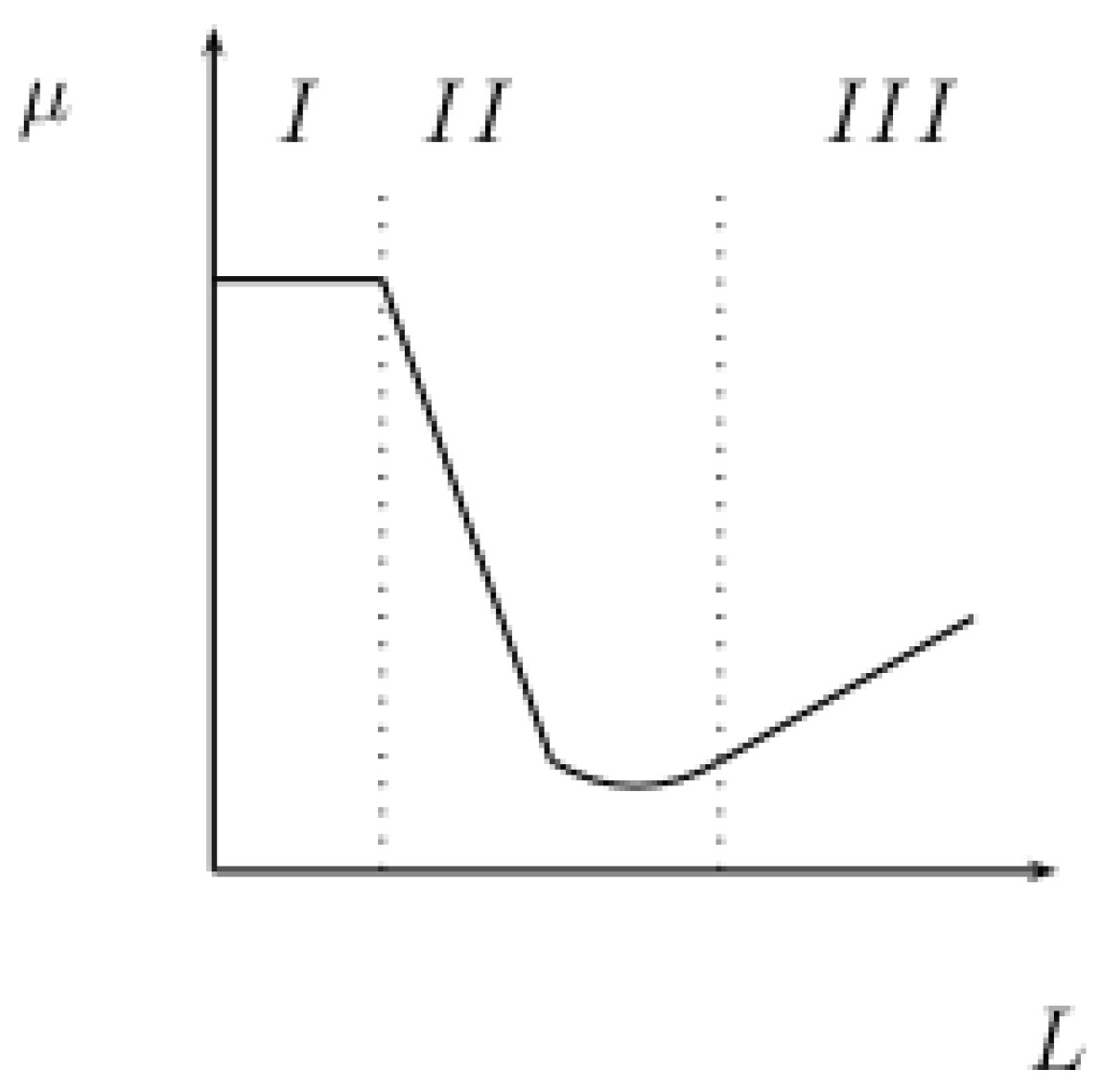
Experiments on wear and friction, as observed in Stribeck’s curve, can provide relations between the friction coefficient μ and the lubricant coefficient L : $\mu =\tau /p$, $L=\eta U/p$ where τ is the shear stress, p the pressure of contact, η the fluid viscosity and U the relative velocity.

Figure 1. Stribeck’s curve.

Figure 1. Stribeck’s curve.

This curve shows three particular regimes: the first regime corresponds to a Coulomb’s friction law with constant coefficient, the second is an unstable regime with a strong decrease of the friction and the third is a linear regime corresponding to a state of mild wear.

These results suggest clearly a strong interaction between debris and the solids in relative motion. The modelization of this interaction can be explored through the evolution of specific internal state variables governing the third-body behaviour.

The simpler approach is made using of theory of mixtures, where the volume fraction of debris plays an important role.

The main purpose of this article is to propose a more general formulation using of thermodynamical considerations on wear phenomena studying the propagation of surfaces or layers inside sound bodies taking account of damage evolution and loss of sound matter. A thermodynamical approach of third body is then introduced and dissipation is analyzed.

For a macroscopic view point the behaviour of the interface is modelized by unit of surface of contact. The density of mass by surface unit is related to the volume fractions of detached particles and plays the role of an internal parameter. The driving force associated to wear is then deduced and criteria of wear are proposed.

Finally, particular situations are studied using some constitutive law of the interface. In each case the dissipation is analysed. The matter loss and the geometry change are determined according to specific criteria and associated laws. Analytical and semi-analytical solutions are presented.

2. General Features on Moving Surfaces and Moving Layers

The wear phenomena due to contact and to relative motion between two solids $V_1$, $V_2$ depend on loading conditions and on material mechanical constitutive laws of the solids in contact. Wear is essentially characterized by a matter loss. Each solid $V_i$ is decomposed into a undamaged part ${\Omega }_i$ and a damaged zone ${\Omega }_{i3}$. The boundary between ${\Omega }_i$ and ${\Omega }_{i3}$ is ${\Gamma }_i={\Gamma }_{i3}$.

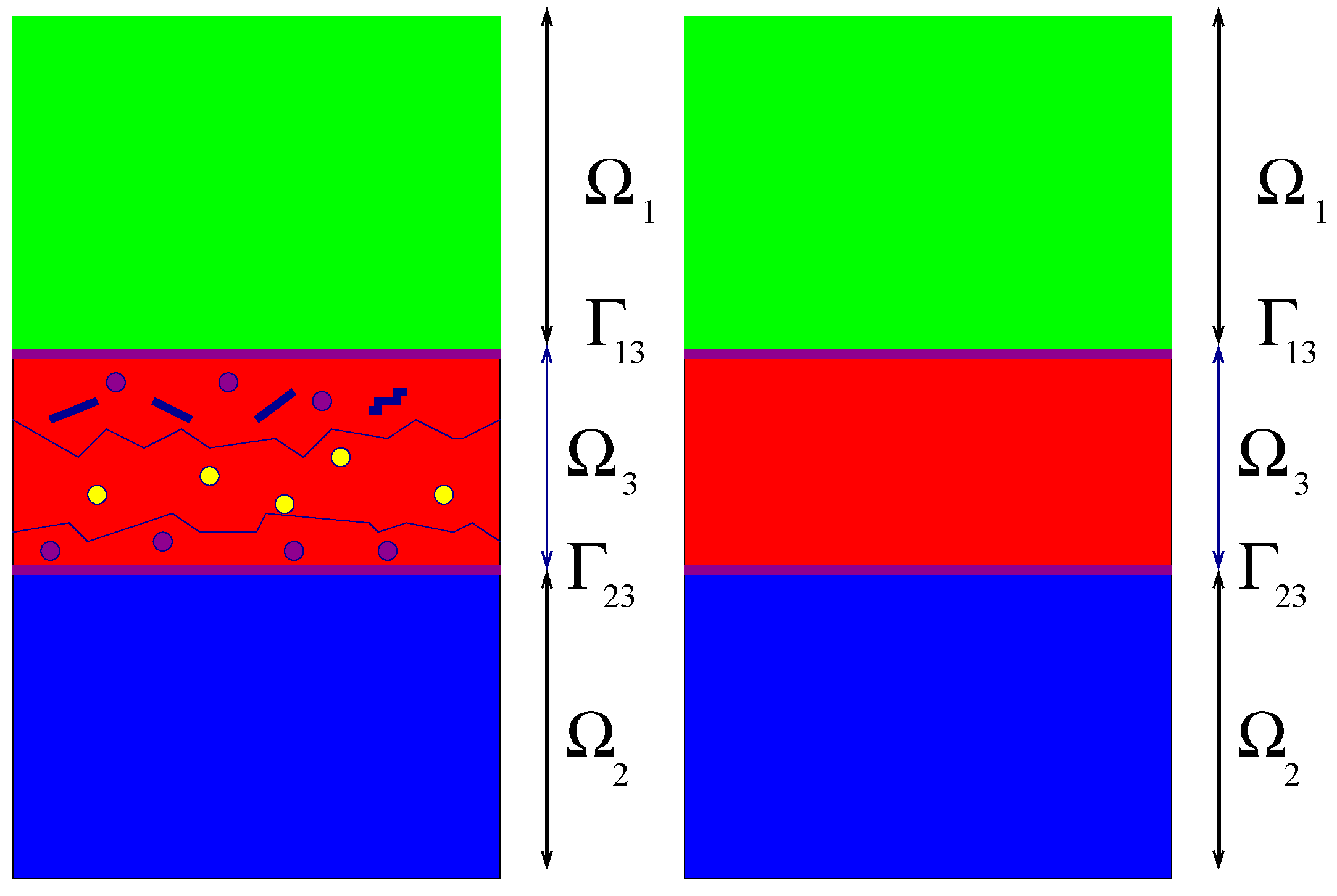
Particles are moved from the solids ${\Omega }_i$ when some criteria are satisfied at the boundaries ${\Gamma }_i$ between ${\Omega }_i$ and a complex medium ${\Omega }_3$ is generated called the interface or the third body.

The third body ${\Omega }_3$ is made of detached particles, damaged zone ${\Omega }_{i3}$ of the two solids as depicted in Figure 2.

Figure 2. The microscopic description of wear process.

Figure 2. The microscopic description of wear process.

The first step of modelization is to characterize the motion of the surface ${\Gamma }_i$. The third body ${\Omega }_3$ is then ${\Omega }_{13}\cup {\Omega }_{23}\cup {\Omega }_{33}$, where ${\Omega }_{33}$ is a complex mixture of detached particles and eventually of a lubricant fluid.

Along the surface ${\Gamma }_{i3}$ the displacement is continuous and the stress vector too. The local behaviour changes from those of the undamaged material ${\Omega }_i$ to those of a damaged solid ${\Omega }_{i3}$. The surface ${\Gamma }_{i3}$ moves with the normal velocity $c_i={\varphi }_i{\underline{\nu }}_i$ in the reference state of the solid, ${\underline{\nu }}_i$ is the outward unit normal vector to ${\Omega }_{i3}$ and then ${\varphi }_i$ is positive. The value of ${\varphi }_i$ is given by a constitutive law, this is a part of the wear description.

This transition can be brutal or diffuse. In the first situation, the transition is governed by the motion of a surface ${\Gamma }_{i3}$ along which the material characteristics endure change by an irreversible process. Due to damage, the elastic moduli in domain ${\Omega }_{i3}$ are lower then those in ${\Omega }_i$, then during this brutal transformation the elastic moduli are discontinuous along ${\Gamma }_{i3}$. These discontinuities contribute to the dissipation by a surface term.

In the second situation, the variation of the quantities is smooth and the quantities remain continuous. The damaged zone ${\Omega }_{i3}$ constitutes a thin layer where the damage and the internal variables vary continuously. The boundary ${\Gamma }_{i3}$ between the undamaged material and the damaged zone is moving but all the mechanical quantities are continuous, the surface term in the dissipation disappears.

Each situation implies different type of dissipation and for each case a driving force associated to the wear process is proposed.

The conditions of loading are chosen such that the inertia effects are small. Extension to dynamical problems uses dynamical concept for the driving force applied for defects motion [8], interface or surface motion [9,10,11,12].

The local constitutive law The state of each body is characterized by the displacement $\underline{u}$, from which the strain field ε is derived. The other parameters are the temperature θ and a set of internal parameters α. The behaviour of $V_i$ is defined by the free energy density ψ as a function of strain ε, the temperature θ and the set of internal parameters α. The mass density of each phase (undamaged and damaged) is the same ρ. The state equations of each phase are

$${\mathit{\sigma }}^r=\rho {\displaystyle \frac{\partial \psi }{\partial \epsilon }},s=-\rho {\displaystyle \frac{\partial \psi }{\partial \theta }},A=-\rho {\displaystyle \frac{\partial \psi }{\partial \alpha }}$$

(1)

The boundary ${\Gamma }_{i3}$, between ${\Omega }_i$ and ${\Omega }_{i3}$, is a perfect interface. The external boundary $\partial {\Omega }_i/{\Gamma }_{i3}$ is decomposed into $\partial V_u$ and $\partial V_T$ on which the displacement ${\underline{u}}^d$ and the loading $T^d$ are prescribed respectively.

The internal state of stresses satisfies the conservation of the momentum

$$div\mathit{\sigma }=0,\mathrm{over}V,\mathit{\sigma }.\underline{n}=T^d,\mathrm{on}\partial V_T,{\left[\mathit{\sigma }\right]}_{{}_{{\Gamma }_i}}.{\underline{\nu }}_i=0,\mathrm{along}{\Gamma }_{i3}$$

(2)

This state σ is decomposed in the reversible part ${\mathit{\sigma }}^r$ and an irreversible part ${\mathit{\sigma }}^{ir}$. The irreversible stresses ${\mathit{\sigma }}^{ir}$ are essentially due to viscosity. In non linear mechanics, the internal state is generally associated with irreversibility. The evolution of internal state must satisfy the second law of thermodynamics. Such requirement is fulfilled by the existence of a potential of dissipation.

Analysis of the dissipation and potential of dissipation The fundamental inequality of thermodynamics implies that the internal production of entropy must be non negative. The equations of state do not provide all the constitutive equations; some complementary laws are necessary to describe the irreversibility. In the total dissipation $D_T$ the contribution of the conduction and those of internal forces must be distinguished.

$$D_T=\mathit{\sigma }:\dot{\epsilon }-\rho (\dot{\psi }+s\dot{\theta })-\frac{q.\nabla \theta }{{\theta }^2}=D_m+D_c\ge 0$$

(3)

The two parts are assumed to be separately non-negative. The mechanical part has the form:

$$D_m=\mathit{\sigma }:\dot{\epsilon }-\rho (\dot{\psi }+s\dot{\theta })\ge 0$$

(4)

and using of equations of state, the thermodynamical forces associated to irreversibility are obtained

$$D_m=(\mathit{\sigma }-{\mathit{\sigma }}^r):\dot{\epsilon }+A.\dot{\alpha }\ge 0$$

(5)

and we recognize the role of the irreversible stresses ${\mathit{\sigma }}^{ir}$.

To determine the evolution of the internal state, relation between velocity and driving forces must be given. These relations must be compatible with the positivity of the internal production of entropy $D_m$.

Let us assume that the local behaviour belongs to the class of the so-called “generalized standard” materials [13]. For this class, a potential of dissipation $d(\dot{\epsilon },\dot{\alpha })$ defines the local irreversibility. The potential d is a convex function of these arguments with a minimum value at the origin. The evolution of the internal state is given by the normality rule:

$$({\mathit{\sigma }}^{ir},A)\in \partial d(\dot{\epsilon },\dot{\alpha })$$

(6)

this means that the subdifferential $\partial d(\dot{\epsilon },\dot{\alpha })$ of d is the set of state $({\mathit{\sigma }}^{ir},A)$ such that:

$$d(\dot{\epsilon },\dot{a})+{\mathit{\sigma }}^{ir}:({\epsilon }^{*}-\dot{\epsilon })+A.({\alpha }^{*}-\dot{\alpha })\le d({\epsilon }^{*},{\alpha }^{*})$$

(7)

for all admissible fields $({\epsilon }^{*},{\alpha }^{*})$. The existence of such a potential for the dissipation ensures the positivity of the entropy production:

$${\mathit{\sigma }}^{ir}:\dot{\epsilon }+A.\dot{a}\ge d(\dot{\epsilon },\dot{\alpha })-d(0,0)\ge 0$$

(8)

2.1. The conservation laws

Classical laws of conservation are written, taking discontinuities into account:

Mass conservation

$$\begin{array}{ccc}\hfill \mathrm{on}& {\Gamma }_{i3},& m_i=\rho c.{\underline{\nu }}_i=\rho {\varphi }_i\hfill \end{array}$$

(9)

$$\begin{array}{ccc}\hfill \mathrm{over}& V_i,& \dot{\rho }+\rho div\left(\underline{v}\right)=0\hfill \end{array}$$

(10)

Momentum conservation

$$\begin{array}{ccc}\hfill \mathrm{on}& {\Gamma }_{i3},& {\left[\mathit{\sigma }\right]}_{{}_{{\Gamma }_i}}.{\underline{\nu }}_i=0\hfill \end{array}$$

(11)

$$\begin{array}{ccc}\hfill \mathrm{over}& V_i,& div\left(\mathit{\sigma }\right)=0\hfill \end{array}$$

(12)

Energy balance

$$\begin{array}{ccc}\hfill \mathrm{on}& {\Gamma }_{i3},& m_i{[\psi +s\theta ]}_{{}_{\Gamma }}-{\underline{\nu }}_i.\mathit{\sigma }.{\left[\underline{v}\right]}_{{}_{{\Gamma }_i}}+{\underline{\nu }}_i.{\left[\underline{q}\right]}_{{}_{{\Gamma }_i}}=0\hfill \end{array}$$

(13)

$$\begin{array}{ccc}\hfill \mathrm{over}& V_i,& \dot{e}=\mathit{\sigma }:\dot{\epsilon }-div\underline{q}\hfill \end{array}$$

(14)

where e is the internal energy $e=w+s\theta$, s is the entropy, $\underline{q}$ the heat flux

Continuity of displacement

$$\mathrm{along}{\Gamma }_{i3},{\left[\underline{u}\right]}_{{}_{{\Gamma }_i}}=0\Rightarrow {\left[\underline{v}\right]}_{{}_{{\Gamma }_i}}+{\varphi }_i{\left[\nabla \underline{u}\right]}_{{}_{{\Gamma }_i}}.{\underline{\nu }}_i=0$$

(15)

Continuity of temperature

$$\mathrm{along}{\Gamma }_{i3},{\left[\theta \right]}_{{}_{{\Gamma }_i}}=0$$

(16)

2.2. On moving interface

To study this problem, the analysis is made on one body $V_i$. The solid is decomposed into ${\Omega }_i$ and ${\Omega }_{i3}$. Along the boundary ${\Gamma }_{i3}$, ${\underline{\nu }}_i$ is the outward unit normal vector to ${\Omega }_{i3}$, c is the normal velocity and ${\varphi }_i$ is the magnitude of c.

When the surface ${\Gamma }_{i3}$ is moving, a mechanical quantity f can suffer a discontinuity ${\left[f\right]}_{{}_{\Gamma }}=f_i-f_{i3}$. The volume $V_i$ is decomposed in two domains, separated by a moving boundary ${\Gamma }_{i3}$. The volume average of f has a rate defined by

$${\displaystyle \frac{d}{dt}}{\int }_{V_i}f\mathrm{d}\Omega ={\int }_{V_i}\dot{f}\mathrm{d}\Omega -{\int }_{{\Gamma }_{i3}}{\left[f\right]}_{{}_{\Gamma }}c.{\underline{\nu }}_i\mathrm{d}S$$

(17)

Entropy production Using the definition of the entropy of the system $S={\int }_{V_i}\rho s\mathrm{d}\Omega$ the second law of thermodynamic is written as

$$\dot{S}-{\int }_{\partial V}{\displaystyle \frac{\underline{q}.\underline{n}}{\theta }}\mathrm{d}S\ge 0$$

(18)

and after integration by part, the value of the volume dissipation $D_T$ is recovered and a surface contribution appears

$${\int }_{{\Gamma }_{i3}}\rho {\left[s\right]}_{{}_{{\Gamma }_i}}{\varphi }_i-{\left[{\displaystyle \frac{\underline{q}}{\theta }}\right]}_{{}_{\Gamma }}.{\underline{\nu }}_i\mathrm{d}S\ge 0$$

(19)

Taking the balance equation of energy and the continuity of temperature into account, the dissipation by unit of surface is obtained

$$D_S={\displaystyle \frac{1}{\theta }}(m_i{\left[\psi \right]}_{{}_{{\Gamma }_i}}-{\underline{\nu }}_i.\mathit{\sigma }.{\left[\underline{v}\right]}_{{}_{{\Gamma }_i}})={\displaystyle \frac{G_i}{\theta }}{\varphi }_i$$

(20)

This dissipation is a linear function of the normal velocity ${\varphi }_i$ of ${\Gamma }_{i3}$. The quantity $G_i$ is the driving force associated to the movement of ${\Gamma }_{i3}$. The displacement is continuous along ${\Gamma }_{i3}$ then the discontinuity ${\left[\nabla \underline{u}\right]}_{{}_{{\Gamma }_i}}$ satisfies the Hadamard’s relation

$${\left[\nabla \underline{u}\right]}_{{}_{{\Gamma }_i}}=\underline{\lambda }\otimes {\underline{\nu }}_i$$

(21)

and the release rate of energy $G_i$ becomes

$$G_i=\rho {\left[\psi \right]}_{{}_{{\Gamma }_i}}-\mathit{\sigma }:{\left[\epsilon \right]}_{{}_{{\Gamma }_i}}$$

(22)

The condition $m_i=0$, which explains that there is no loss of matter, induces that ${\varphi }_i=0$ then there is no discontinuity ${\left[\underline{v}\right]}_{{}_{{\Gamma }_i}}=0$, so there is no dissipation along the surface ${\Gamma }_{i3}$, because this surface does not move.

Interface propagation law To control the matter loss, a criterion based on $G_i$ can be formulated. For example, we can considered a Griffith’s type law for the propagation of the moving interface

$$G_i-G_c\le 0,{\varphi }_i\ge 0,(G_i-G_c){\varphi }_i=0$$

(23)

When the interface moves hence $G_i=G_c$, this quantity must be conserved during the motion.

Convected differentiation To study the evolution of the mechanical state around the moving surface ${\Gamma }_{i3}$ a convected derivative of any mechanical quantity f is needed. A point ${\underline{X}}_{\Gamma }$ is on ${\Gamma }_{i3}$ if its coordinates satisfy the scalar equation:

$$S({\underline{X}}_{\Gamma },t)=0$$

(24)

It is well known that the gradient $\nabla S({\underline{X}}_{\Gamma },t)=\left|\right|\nabla S\left|\right|{\underline{\nu }}_i$ is normal to the surface. At time $t+dt$ the point ${\underline{X}}_{\Gamma }$ comes in ${\underline{X}}_{\Gamma }+{\varphi }_i{\underline{\nu }}_i({\underline{X}}_{\Gamma },t)dt$ and

$$S(X+{\varphi }_i{\underline{\nu }}_{i}dt,t+dt)=0\to {\displaystyle \frac{\partial S}{\partial X}}.{\varphi }_i{\underline{\nu }}_i+{\displaystyle \frac{\partial S}{\partial t}}=0$$

(25)

For any function $f({\underline{X}}_{\Gamma },t),{\underline{X}}_{\Gamma }\in {\Gamma }_{i3}$, the convected derivative of f in the movement of ${\Gamma }_{i3}$ is

$$D_{\Gamma }f({\underline{X}}_{\Gamma },t):=\underset{dt\to 0}{lim}{\displaystyle \frac{f({\underline{X}}_{\Gamma }+{\varphi }_i{\underline{\nu }}_{i}dt,t+dt)-f({\underline{X}}_{\Gamma },t)}{dt}}$$

(26)

In particular, the evolution of the middle surface satisfies

$$D_{\Gamma }S({\underline{X}}_{\Gamma },t)=0$$

(27)

and the convected derivatives of ${\underline{X}}_{\Gamma }$ and ${\underline{\nu }}_i$ are

$$D_{\Gamma }{\underline{X}}_{\Gamma }={\varphi }_i{\underline{\nu }}_i,D_{\Gamma }{\underline{\nu }}_i={\underline{\nu }}_i.\nabla \left({\varphi }_i{\underline{\nu }}_i\right)$$

(28)

The convected derivative is useful for write the Hadamard’s equation of compatibility: for any continuous function f along ${\Gamma }_{i3}$

$${\left[f\right]}_{{}_{{\Gamma }_i}}=0\Rightarrow D_{\Gamma }{\left[f\right]}_{{}_{{\Gamma }_i}}={\left[D_{\Gamma }f\right]}_{{}_{{\Gamma }_i}}=0$$

(29)

For the displacement, we have

$${\left[\underline{u}\right]}_{{}_{{\Gamma }_i}}=\underline{u}({\underline{X}}_{\Gamma }^{+},t)-\underline{u}({\underline{X}}_{\Gamma }^{-},t)=0$$

(30)

The convected derivative of $\underline{u}({\underline{X}}_{\Gamma }^{+},t)={\underline{u}}^{+}$ and of $\underline{u}({\underline{X}}_{\Gamma }^{-},t)={\underline{u}}^{-}$ are given by

$$D_{\Gamma }{\underline{u}}^{\pm }={\displaystyle \frac{\partial \underline{u}}{\partial t}}({\underline{X}}_{\Gamma }^{\pm },t)+{\varphi }_i\nabla \underline{u}({\underline{X}}_{\Gamma }^{\pm },t).{\underline{\nu }}_i$$

(31)

the classical relation on discontinuity is recovered as

$${\left[\underline{v}\right]}_{{}_{{\Gamma }_i}}+{\varphi }_i{\left[\nabla \underline{u}\right]}_{{}_{{\Gamma }_i}}.{\underline{\nu }}_i={\left[D_{\Gamma }\underline{u}\right]}_{{}_{{\Gamma }_i}}=0$$

(32)

Consistency condition The law of propagation shows that the condition ${\varphi }_i\ne 0$ implies $G_i=G_c$, that relation is conserved during the propagation. The consistency condition associated with the Griffith’s propagation law is then written at point $s\in {\Gamma }_{i3}$ where $G_i=G_c$ in the form

$${\varphi }_i\left(s\right)\ge 0,\forall {\varphi }^{*}\left(s\right)\ge 0,({\varphi }_i\left(s\right)-{\varphi }^{*}\left(s\right))D_{\Gamma }\left(G_i\right)\ge 0$$

(33)

this ensures that ${\varphi }_i\ge 0$ if $D_{\Gamma }\left(G_i\right)=0$. This condition determines the velocity ${\varphi }_i({\underline{X}}_{\Gamma },t)$ ; the surface equation is then implicitly defined by the condition $G_i({\underline{X}}_{\Gamma },t)=G_c$.

This description is based on the fact that the transition between the initial solid and the damaged material is brutal, that transition induces discontinuities.

2.3. On moving layer

The situation of diffuse damage is now considered. For example, a damage constitutive law governed by a continuous scalar function d is assumed and a free energy is taken as

$$\psi (\epsilon ,d)=(1-d){\psi }_o\left(\epsilon \right)=(1-d){\displaystyle \frac{1}{2}}\epsilon :{\mathbb{C}}_o:\epsilon ,\mathit{\sigma }=(1-d){\mathbb{C}}_o:\epsilon$$

(34)

the damage parameter varies from 0 (no damage) to 1 (totally damaged). Over ${\Omega }_i$, $d=0$ and d varies continuously from 0 to 1 over ${\Omega }_{i3}$.

In this description along the surface ${\Gamma }_{i3}$, between sound material and damaged zone, $d=0$. The stress vector (${\left[\mathit{\sigma }\right]}_{{}_{{\Gamma }_i}}.{\underline{\nu }}_i=0$), the displacement and the elastic moduli are continuous quantities. These properties induce that $\nabla \underline{u}$ is continuous and so the energy release rates $G_i$ is zero along the surface ${\Gamma }_{i3}$. The previous results on dissipation must be revisited. The loss of matter is governed by the motion of the surface $d(x,t)=1$.

The volume $V_i$ is decomposed as previously, but now the displacement and the internal parameters are continuous along the surface ${\Gamma }_{i3}$. Inside the domain ${\Omega }_{i3}$, the evolution of a mechanical quantity $f(\epsilon ,\alpha )$ function of the strain ε and of the set of internal parameters α must be characterized. The volume average of f is decomposed as

$$F={\int }_{{\Omega }_i}f(\epsilon ,\alpha )\mathrm{d}\Omega +{\int }_{{\Omega }_{i3}}f(\epsilon ,\alpha )\mathrm{d}\Omega$$

(35)

and has a time-derivative expressed in term of a classical time derivative in ${\Omega }_i$ and a convected derivative on ${\Omega }_{i3}$. Convective derivative is useful to describe hypothesis of self-similarity process in the damaged zone during the wear.

The domain ${\Omega }_{i3}$ evolves simultaneously with two surfaces: one is ${\Gamma }_{i3}$ associated with the boundary $d(x,t)=0$ and the other is ${\Gamma }_o$ along which $d(x,t)=1$.

A point $\underline{x}$ in ${\Omega }_{i3}$ is locally defined by it’s normal projection ${\underline{X}}_{\Gamma }$ on the surface ${\Gamma }_{i3}$ and the normal coordinate z along the unit normal vector ${\underline{\nu }}_i$. The thickness of the layer is $H(S,t)$ and $0\le z\le H$.

$$\underline{x}={\underline{X}}_{\Gamma }-z{\underline{\nu }}_i$$

(36)

When the surface ${\Gamma }_{i3}$ moves with the normal velocity ${\varphi }_i$, the local frame ${\underline{\tau }}_i,{\underline{\nu }}_i$ moves simultaneously. For example a 2D motion of a curve satisfies the geometric relations

$${\displaystyle \frac{\mathrm{d}{\underline{X}}_{\Gamma }}{\mathrm{d}S}}={\underline{\tau }}_i,D_{\Gamma }{\underline{\tau }}_i=-{\displaystyle \frac{\mathrm{d}{\varphi }_i}{\mathrm{d}S}}{\underline{\nu }}_i,D_{\Gamma }{\underline{\nu }}_i={\displaystyle \frac{\mathrm{d}{\varphi }_i}{\mathrm{d}S}}{\underline{\tau }}_i,{\displaystyle \frac{\mathrm{d}{\gamma }_i}{\mathrm{d}S}}={\displaystyle \frac{{\mathrm{d}}^2{\varphi }_i}{\mathrm{d}{S}^2}}+{\gamma }_i^2{\varphi }_i$$

(37)

where ${\gamma }_i$ is the curvature of the surface ${\Gamma }_{i3}$ at point S, ${\underline{\nu }}_i$ the normal unit vector et ${\underline{\tau }}_i$ the tangent unit vector to the curve. It can be noticed that

$${\displaystyle \frac{\mathrm{d}\underline{x}}{\mathrm{d}S}}={\underline{\tau }}_i-z{\displaystyle \frac{\mathrm{d}{\underline{\nu }}_i}{\mathrm{d}S}}=(1-{\gamma }_{i}z){\underline{\tau }}_i$$

(38)

the elementary length is function of the curvature

$$\mathrm{d}s=j\left(\underline{x}\right)\mathrm{d}S$$

(39)

in the reference coordinates $({\underline{X}}_{\Gamma },z)$. Similar relations exist for a surface motion.

The point $\underline{x}$ has a convected derivative

$$D_{\Gamma }\underline{x}\left(z\right)={\varphi }_i{\underline{\nu }}_i-z{D}_{\Gamma }{\underline{\nu }}_i$$

(40)

During the motion, the thickness evolves and the velocity of the point $M=\underline{x}\left(H\right)$ is

$$D_{\Gamma }M=D_{\Gamma }\underline{x}\left(H\right)-\dot{H}{\underline{\nu }}_i$$

(41)

The evolution of each term of F can now be given.

$$\begin{array}{ccc}& & {\displaystyle \frac{d}{dt}}({\int }_{{\Omega }_i}f\mathrm{d}\Omega )={\int }_{{\Omega }_i}{\displaystyle \frac{df}{dt}}\mathrm{d}\Omega -{\int }_{{\Gamma }_{i3}}f{D}_{\Gamma }\underline{x}\left(o\right).{\underline{\nu }}_i\mathrm{d}S\hfill \end{array}$$

(42)

$$\begin{array}{ccc}& & {\displaystyle \frac{d}{dt}}({\int }_{{\Omega }_{i3}}f\mathrm{d}\Omega )={\int }_{{\Omega }_{i3}}{\displaystyle \frac{df}{dt}}\mathrm{d}\Omega -{\int }_{{\Gamma }_o}f{D}_{\Gamma }M.{\underline{\nu }}_H\mathrm{d}S+{\int }_{{\Gamma }_{i3}}f{D}_{\Gamma }x\left(o\right).{\underline{\nu }}_i\mathrm{d}S\hfill \end{array}$$

(43)

$$\begin{array}{ccc}& & \dot{F}={\int }_{{\Omega }_i}{\displaystyle \frac{df}{dt}}\mathrm{d}\Omega +{\int }_{{\Gamma }_{i3}}{\left[f\right]}_{{}_{\Gamma }}{D}_{\Gamma }x\left(o\right).{\underline{\nu }}_i\mathrm{d}S+{\int }_{{\Omega }_{i3}}{\displaystyle \frac{df}{dt}}\mathrm{d}\Omega +{\int }_{{\Gamma }_o}f{D}_{\Gamma }M.{\underline{\nu }}_H\mathrm{d}S\hfill \end{array}$$

(44)

In these expressions, $D_{\Gamma }\underline{x}\left(o\right)={\varphi }_i{\underline{\nu }}_i,D_{\Gamma }M={\varphi }_H{\underline{\nu }}_H={\varphi }_i{\underline{\nu }}_i-D_{\Gamma }\left(H{\underline{\nu }}_i\right)$.

The function f is continuous along Γ, then there is no contribution of discontinuities on the time derivative of F, then

$$\dot{F}={\int }_{{\Omega }_i}{\displaystyle \frac{df}{dt}}\mathrm{d}\Omega +{\int }_{{\Omega }_{i3}}{\displaystyle \frac{df}{dt}}\mathrm{d}\Omega +{\int }_{{\Gamma }_o}f{D}_{\Gamma }M.{\underline{\nu }}_H\mathrm{d}S$$

(45)

The only surface contribution is due to the flux of matter along the surface ${\Gamma }_o$. Along ${\Gamma }_o$, the loss matter occurs simultaneously with the full damage $d=1$.

Over ${\Omega }_{i3}$, the convected derivative of f is used

$$D_{\Gamma }f={\displaystyle \frac{df}{dt}}+\nabla f.D_{\Gamma }\underline{x}$$

(46)

and we have

$${\int }_{{\Omega }_{i3}}{D}_{\Gamma }f+ftr\left(\nabla D_{\Gamma }\underline{x}\right)\mathrm{d}\Omega ={\int }_{{\Omega }_{i3}}{\displaystyle \frac{df}{dt}}\mathrm{d}\Omega +{\int }_{\partial {\Omega }_{i3}}f{D}_{\Gamma }\underline{x}.\underline{\nu }\left(\underline{x}\right)\mathrm{d}S$$

(47)

then the rate of F is finally

$$\dot{F}={\int }_{{\Omega }_i}{\displaystyle \frac{df}{dt}}\mathrm{d}\Omega +{\int }_{{\Omega }_{i3}}\left(D_{\Gamma }f+f\mathrm{tr}\left(\nabla D_{\Gamma }\underline{x}\right)\right)\mathrm{d}\Omega -{\int }_{{\Gamma }_o}f\dot{H}{\underline{\nu }}_i.{\underline{\nu }}_H\mathrm{d}S$$

(48)

The global dissipation is expressed using these expressions.

Analysis of dissipation The dissipation has the classical expression

$$D_m={\int }_{\partial V}\underline{n}.\mathit{\sigma }.\underline{v}\mathrm{d}S-{\displaystyle \frac{\mathrm{d}}{\mathrm{d}t}}{\int }_V\psi (\epsilon ,\alpha )\mathrm{d}\Omega$$

(49)

as previously we have

$$D_m={\int }_{{\Omega }_{i3}}A.\dot{\alpha }+{\mathit{\sigma }}_{ir}:\dot{\epsilon }\mathrm{d}\Omega +{\int }_{{\Gamma }_o}\psi D_{\Gamma }M.{\underline{\nu }}_H\mathrm{d}S$$

(50)

The dissipation contains to terms, one in the volume and the last one defined on the surface. In the transient phase this terms is zero, because the material in ${\Omega }_{i3}$ is only partially damaged $d<1$, then $D_{\Gamma }M.{\underline{\nu }}_H=0$. When rupture occurs, this term contributes to the dissipation, the value of energy at point $d=1$ is lost.

Some others expressions for dissipation can be formulated.

Others expressions of dissipation Introducing the local Eshelby momentum tensor P

$$\mathit{P}=\psi \mathbf{1}-\mathit{\sigma }.\nabla \underline{u}$$

(51)

This tensor satisfies the relations

$$div{\mathit{P}}^T=-A:\nabla \alpha -{\mathit{\sigma }}_{ir}:\nabla \epsilon ,in{\Omega }_{i3},\underline{\nu }.{\left[\mathit{P}\right]}_{{}_{{\Gamma }_i}}=0,along{\Gamma }_{i3}$$

(52)

And using the convected frame with ${\Omega }_{i3}$ with the velocity $D_{\Gamma }\underline{x}$, the dissipation is rewritten as

$$\begin{array}{ccc}\hfill D_m& =& {\int }_{{\Omega }_{i3}}(A.D_{\Gamma }\alpha +{\mathit{\sigma }}_{ir}:D_{\Gamma }\epsilon )\mathrm{d}\Omega \hfill \\ & -& {\int }_{{\Omega }_{i3}}\mathit{P}:\left(\nabla D_{\Gamma }x\right)\left(z\right)\mathrm{d}\Omega +{\int }_{\partial {\Omega }_{i3}}\underline{\nu }.\mathit{P}.D_{\Gamma }x\left(z\right)\mathrm{d}S\hfill \\ & +& {\int }_{{\Gamma }_o}\psi \dot{H}{\underline{\nu }}_i.{\underline{\nu }}_H\mathrm{d}S\hfill \end{array}$$

(53)

This expression has a great interest when local conditions of the stationarity of the steady state is realized. If the damage d is a function of the distance z to the curve ${\Gamma }_{i3}$ the local stationarity is expressed as

$$D_{\Gamma }d=\dot{d}+{\varphi }_i\nabla d.{\underline{\nu }}_i=0$$

(54)

and for local stationarity, $D_{\Gamma }\alpha =0$.

Comments on local stationarity If Y is the driving force associated to d, then the contribution of damage to dissipation is

$$\begin{array}{ccc}\hfill D_d={\int }_{{\Omega }_{i3}}Y\dot{d}\mathrm{d}\Omega & =& -{\int }_{{\Omega }_{i3}}Y\nabla d.{\underline{\nu }}_{i}j\left(\underline{x}\right)dz{\varphi }_i\left(S\right)\mathrm{d}S\hfill \end{array}$$

(55)

$$\begin{array}{ccc}& =& -{\int }_{{\Gamma }_{i3}}{\int }_{H\left(S\right)}\left(Y\left(\underline{x}\right)\nabla d.{\underline{\nu }}_{i}j\left(\underline{x}\right)\right)dz{\varphi }_i\left(S\right)\mathrm{d}S\hfill \end{array}$$

(56)

Therefore, if the distribution of $\nabla d$ is known inside the layer, the average value $\overline{G_i}$ is the driving force associated to the velocity ${\varphi }_i$,

$${\overline{G}}_i=-{\int }_{H\left(S\right)}\left(Y\left(\underline{x}\right)\nabla d.{\underline{\nu }}_{i}j\left(\underline{x}\right)\right)dz$$

(57)

The quantity $j\left(\underline{x}\right)$ takes the shape of the layer into account and it defines the measure of area at $\underline{x}$ with respect to the measure of area at ${\underline{X}}_{\Gamma }$ so that

$$\mathrm{d}\Omega \left(\underline{x}\right)=\mathrm{d}sdz=j\left(\underline{x}\right)\mathrm{d}Sdz$$

(58)

Assuming now that the profile $d\left(z\right)$ is a given function, the propagation law is generalized as

$$({\overline{G}}_i-G_c){\varphi }_i=0,{\varphi }_i\ge 0,{\overline{G}}_i-G_c\le 0$$

(59)

Combining the hypothesis of stationarity and an imposed profile for d, the thickness H is given, the ${\Gamma }_o$ interface is moving with the normal velocity ${\varphi }_i$ of ${\Gamma }_{i3}$, when $-{\int }_H\nabla d.{\underline{\nu }}_{i}j\left(\underline{x}\right)dz=1$.

In this case, the iso-d curves are orthogonal to the normal ${\underline{\nu }}_i$ and each iso-d curve has the same velocity ${\varphi }_i$.

3. The Macroscopic Interface Study

From a macroscopic point of view, it is not necessary to model the microscopic behaviour which occurs in ${\Omega }_3$. Micromechanical considerations can be useful in order to describe in a realistic manner the behaviour of the interface. This type of analysis can provide a relevant interface law at the mesoscopic level and at macroscopic scale too. The multi scale approach of the interface is based on fundamental characteristics at three different scales:

• At the microscopic scale, the contact between asperities govern the wear mechanisms. Some studies with plastic strains and with micro cracks propagation have been tempted [5,14]. These are the fundamental ideas of the decomposition of ${\Omega }_3$ in ${\Omega }_{13}\cup {\Omega }_{33}\cup {\Omega }_{23}$.
• At the mesoscopic scale, this is the description of the third body. This model was proposed in [1] developed by [15] and [16]. The local physics is that ${\Omega }_{i3}$ is a porous medium. In ${\Omega }_{33}$ the solid particles are in suspension forming a shear layer as inside a viscous fluid flow. This point is developed in [3]. In other situations, a very large plastic shear deformation is present, so the profile of local deformation in this thin layer depends strongly on the loading conditions.
• The macroscopic modelling is based on models of friction law which are depending on parameters to account of the evolution of the interface. These models can be inferred from the smaller scale by some averaging technics as those proposed under local stationarity hypothesis.

Some other studies are founded on cyclic loading taking account of cyclic asymptotic behaviour of elastoplastic materials generalised to the theory of damage in mechanics [17].

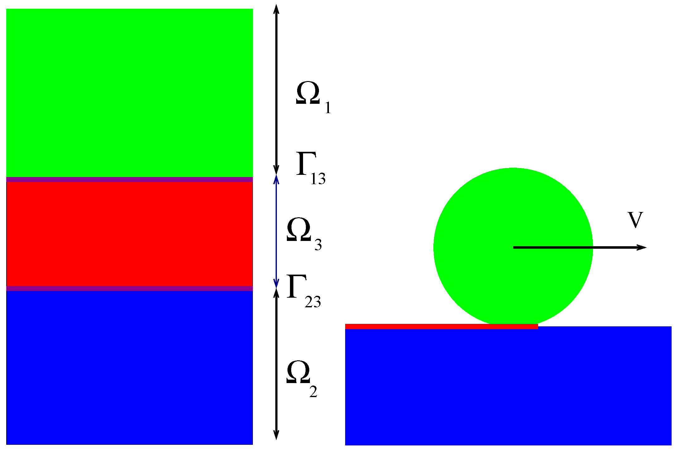
The system of two bodies in relative motion separated by the third body ${\Omega }_3$ is considered. As previously in each domain the local behaviour is described by a free energy ψ and a potential d of dissipation. The dissipation is considered only for domain ${\Omega }_3$. So the behaviour in ${\Omega }_1$ and ${\Omega }_2$ is reversible. Therefore dissipation is concentrate into the interface.

The proposed description is depicted in Figure 3.

Figure 3. The transition from microscopic to mesoscopic description of wear process.

Figure 3. The transition from microscopic to mesoscopic description of wear process.

Sharp transition At the mesoscopic level, the dissipation is given by

$$D={\int }_S{\int }_H{d}_{3}dz+\sum _i{\displaystyle \frac{1}{{\theta }_i}}{\varphi }_i({\left[\rho \psi \right]}_{{}_{{\Gamma }_i}}-\mathit{\sigma }:{\left[\epsilon \right]}_{{}_{{\Gamma }_i}})j_i\mathrm{d}S$$

(60)

where ${\left[f\right]}_{{}_{{\Gamma }_i}}=f_i-f_3$, and $d_3$ is the volume dissipation due to the irreversibility processes inside ${\Omega }_3$:

$$d_3=-{\displaystyle \frac{\underline{q}.\nabla \theta }{{\theta }^2}}+{\displaystyle \frac{1}{\theta }}(\mathit{\sigma }:\nabla \underline{v}-\rho (\dot{\psi }+s\dot{\theta }))$$

(61)

Comments If matter loss occurs, $m_1$ or $m_2$ is positive, then the corresponding discontinuity ${\left[\underline{v}\right]}_{{}_{{\Gamma }_i}}$ exists too and the local quantity $G_i=m_i{(\left[\psi \right]}_{{}_{{\Gamma }_i}}-\mathit{\sigma }:{\left[\epsilon \right]}_{{}_{{\Gamma }_i}}$) is positive. There is a dissipation due to the loss of material: that is a characterization of wear.

The volume dissipation $d_3$ contains two contributions, one is due to heat conduction, the other is associated to mechanical irreversibility. This contribution can be associated with the viscosity of the fluid which carry the detached particle. When the shear reaches a critical value ${\tau }_c$ the velocity field inside the interface is reduced to a gliding motion $\underline{v}=U/Hz{\underline{e}}_x$ and the dissipation in the mesoscopic scale is evaluated as

$$D=-{\int }_{\Omega }{\displaystyle \frac{\underline{q}.\nabla \theta }{{\theta }^2}}\mathrm{d}\Omega +{\int }_S({\displaystyle \frac{{\tau }_{c}U}{\theta }}+\sum _i{\displaystyle \frac{G_i\varphi }{{\theta }_i}})\mathrm{d}S$$

(62)

The second term is due to the viscoplasticity governed by the yield stress ${\tau }_c$, it plays the role of friction [18,19].

The control of the wear dissipation obeys to the normality rule

$$G_i-G_c^i\le 0,{\varphi }_i\ge 0,(G_i-G_c^i){\varphi }_i=0$$

(63)

This simple description is based on the brutal transition on the mechanical characteristic from initial material to a damaged one. The interface ${\Gamma }_{i3}$ moves according to this normality rule.

Diffuse damage Consider now that ${\Omega }_{i3}$ is a zone of diffuse damage. The description of damage can be made with a smooth transition governed by a damage parameter d in ${\Omega }_{i3}$, a set of internal parameters α, which contains the plastic strain ${\epsilon }_p$. For example a free energy of the form

$${\psi }_i(\epsilon ,\alpha ,d)={\displaystyle \frac{1}{2}}(\epsilon -\alpha ):{\mathbb{C}}_i\left(d\right):(\epsilon -\alpha )+{\psi }_b(d,\alpha )$$

(64)

is considered. In this case, the damage parameter governs continuously the change of moduli of elasticity and it describes the degradation of the stiffness.

As previously, the state equations are given by

$${\mathit{\sigma }}_r={\mathbb{C}}_i\left(d\right):(\epsilon -\alpha ),A={\mathit{\sigma }}_r-{\displaystyle \frac{\partial W}{\partial \alpha }},Y=-{\displaystyle \frac{\partial {\psi }_i}{\partial d}}$$

(65)

and a potential of dissipation $d_i(\dot{\epsilon },\dot{\alpha },\dot{d})$ is given so that

$${\mathit{\sigma }}_{ir}={\displaystyle \frac{\partial d_i}{\partial \dot{\epsilon }}},A={\displaystyle \frac{\partial d_i}{\partial \dot{\alpha }}},Y={\displaystyle \frac{\partial d_i}{\partial \dot{d}}}$$

(66)

The thickness of the interface ${\Omega }_3={\Omega }_{13}\cup {\Omega }_{33}\cup {\Omega }_{23}$ is $H=H_1+H_3+H_2$. At this stage all possible choice for the local constitutive behaviour can be used. And literature provide many papers on this subject with computational results. But the main difficulty is to determine the physical characteristics of the behaviour at this scale.

A macro level approach based on this local description can be tempted to understand the specific structure of the thin layer and to estimate some necessary parameters to a relevant description of the mechanisms inside the interface.

4. A Macrolevel Approach

The preceding sections emphasise the fact that in a more general global approach, we can tempt to characterize the thin layer behaviour by considering it is in a state of equilibrium under given conditions applied to ${\Gamma }_{i3}$. Then the behaviour of the thin layer can be considered as affected to a surface Γ, by considering that the thickness is an infinitesimal quantity compared to a characteristic length of the bodies in interaction. Time derivatives of integral of varying surface or volume domains are studied in [20]. Some such results are used here to express the dissipation.

The interface ${\Omega }_3$ is a thin layer composed by ${\Omega }_{13}\cup {\Omega }_{33}\cup {\Omega }_{23}$. The geometry of the layer is described by its middle surface Γ and the thickness $H=2h$ at each point of this surface.

The free energy ${\psi }_s$ per unit of area of the middle surface Γ of the layer is defined by

$${\psi }_s={\displaystyle \frac{1}{{\rho }_s}}{\int }_H\rho \left(\underline{x}\right){\psi }_3(\epsilon \left(\underline{x}\right),\alpha \left(\underline{x}\right))j\left(\underline{x}\right)dz$$

(67)

$\underline{x}={\underline{X}}_{\Gamma }+z\underline{\nu }$, ${\underline{X}}_{\Gamma }$ is the position of the middle surface, z is the normal coordinate $-h\le z\le h$, the middle surface has a curvature κ, and $j\left(\underline{x}\right)$ is the variation of area surface due to curvature with respect to the middle surface coordinates. The local volume is then $\mathrm{d}\Omega =j\left(\underline{x}\right)dz\mathrm{d}S$.

The mass ${\rho }_s$ by unit of area is defined by

$${\rho }_s={\int }_H\rho \left(\underline{x}\right)j\left(\underline{x}\right)dz$$

(68)

The mass of the overall system is not conserved. The mass loss ${\rho }_i{\varphi }_i$ from ${\Omega }_i$ is added to ${\Omega }_3$ hence we obtain

$${\displaystyle \frac{d}{dt}}{\int }_{{\Omega }_{i3}}\rho \mathrm{d}\Omega ={\displaystyle \frac{d}{dt}}{\int }_{\Gamma }{\rho }_s\mathrm{d}S={\int }_{\Gamma }\left[\right|\rho \varphi j\left|\right]\mathrm{d}S$$

(69)

with $\left[\right|\rho \varphi j\left|\right]={\rho }_1{\varphi }_1{j}_1+{\rho }_2{\varphi }_2{j}_2$. But in the same time, a flux of matter is present in the tangent plane of Γ with the velocity ${\underline{C}}_s$ Then the rate of the surface density is given by

$${\displaystyle \frac{d}{dt}}{\int }_{\Gamma }{\rho }_s\mathrm{d}S={\int }_{\Gamma }(D_{\Gamma }{\rho }_s-\varphi {\rho }_s\gamma )\mathrm{d}S-{\int }_{\partial \Gamma }{\rho }_s{\underline{C}}_s.\underline{n}dl={\int }_{\Gamma }\left[\right|\rho \varphi j\left|\right]\mathrm{d}S$$

(70)

This contributes locally to the matter flux. Assuming that the conservation is locally true, we have

$$D_{\Gamma }{\rho }_s-\varphi {\rho }_s\gamma -{div}_s\left({\rho }_s{\underline{C}}_s\right)=\left[\right|\rho \varphi j\left|\right]$$

(71)

The local problem The layer is in equilibrium with external loading and contact conditions. The displacement is continuous on ${\Gamma }_i$ , the surface energy ${\psi }_s$ depends upon the given displacements along ${\Gamma }_i$. The other parameters are a set of internal parameters $\alpha ({\underline{X}}_{\Gamma },z)$, the thickness $H\left({\underline{X}}_{\Gamma }\right)$ and the temperature. The local strain ε derives from the displacement ${\underline{u}}_3$. The displacement is continuous along the interfaces ${\Gamma }_i$ then

$${\underline{u}}_1({\underline{x}}_1,t)={\underline{u}}_3({\underline{X}}_{\Gamma }+h\underline{\nu },t),{\underline{u}}_2({\underline{x}}_2,t)={\underline{u}}_3({\underline{X}}_{\Gamma }-h\underline{\nu },t),h=H/2$$

(72)

Then, it is obvious that the surface free energy is a function of ${\underline{u}}_i({\underline{x}}_i,t)$ and of the thickness H.

Time derivatives of integral of varying surface or volume domains are studied in [20]. Some such results are used here to express the dissipation.

The strain is rate is $\dot{\epsilon }={\displaystyle \frac{1}{2}}(\nabla \underline{v}+{\nabla }^T\underline{v})$, where $\underline{v}=\dot{\underline{u}}$. The dissipative function $D_s$ associated to the local potential $d_3=d(\dot{\epsilon },\dot{\alpha })$ is defined by the average

$${\rho }_s{D}_s({\underline{v}}_1,{\underline{v}}_2,\dot{\alpha })={\int }_H\rho \left(\underline{x}\right)d(\dot{\epsilon }\left(\underline{x}\right),\dot{\alpha })j\left(\underline{x}\right)dz$$

(73)

We consider that the behaviour inside ${\Omega }_i$ is reversible. The steady state equations over ${\Omega }_i$ are then

$$\begin{array}{ccc}\hfill \mathit{\sigma }& =& {\rho }_i{\displaystyle \frac{\partial {\psi }_i}{\partial \epsilon }},div\mathit{\sigma }=0,\hfill \\ \hfill \epsilon & =& {\displaystyle \frac{1}{2}}(\nabla \underline{u}+{\nabla }^T\underline{u})\hfill \end{array}$$

For the interface, we have

$${\underline{T}}_i^r={\rho }_s{\displaystyle \frac{\partial {\psi }_s}{\partial {\underline{u}}_i}},A=-{\rho }_s{\displaystyle \frac{\partial {\psi }_s}{\partial \alpha }},G_s=-{\rho }_s{\displaystyle \frac{\partial {\psi }_s}{\partial H}}$$

(74)

where ${\underline{T}}_i^r$ is the reversible tension along the interface. The balance momentum equations using of the local behaviour is given by

$${\underline{\nu }}_i.\mathit{\sigma }{j}_i={\underline{T}}_i^r+{\underline{T}}_i^{ir}={\rho }_s({\displaystyle \frac{\partial {\psi }_s}{\partial {\underline{u}}_i}}+{\displaystyle \frac{\partial D_s}{\partial {\underline{v}}_i}})$$

(75)

and the complementary laws are

$$A=-{\rho }_s{\displaystyle \frac{\partial D_s}{\partial \dot{\alpha }}},{\underline{T}}_i^{ir}={\rho }_s{\displaystyle \frac{\partial D_s}{\partial {\underline{v}}_i}}$$

(76)

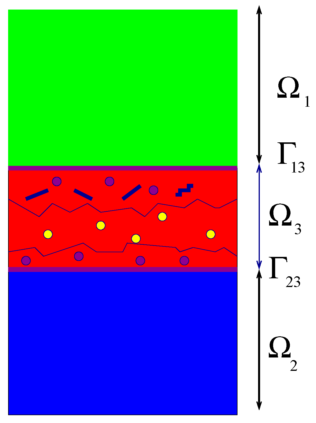
Figure 4. The transition from mesoscopic description to macroscopic description of wear process.

Figure 4. The transition from mesoscopic description to macroscopic description of wear process.

The normal ${\underline{\nu }}_i$ along the interface ${\Gamma }_{i3}$ is not the normal to the middle surface because h depends on ${\underline{X}}_{\Gamma }$.

The macroscopic description as depicted on 4 ignores the details at the microscopic level.

The local thickness $H\left({\underline{X}}_{\Gamma }\right)=2h$ is obviously the relevant parameter geometrically associated with the interface, while the internal parameters govern the physical properties of the layer. For example, the set of volume fraction of debris from materials 1 and 2 are such parameters.

Analysis of dissipation The global dissipation is derived from the macroscopic description. It is useful to introduce the global free energy $\mathcal{P}$ of the tribologic system

$$\mathcal{P}={\int }_{{\Omega }_i}{\rho }_i{\psi }_i(\epsilon \left(\underline{u}\right),\alpha )\mathrm{d}\Omega +{\int }_{\Gamma }{\rho }_s{\psi }_s({\underline{u}}_1,{\underline{u}}_2,h,\alpha )\mathrm{d}S$$

(77)

The rate of the free energy is then

$$\frac{\mathrm{d}\mathcal{P}}{\mathrm{d}t}=\frac{\mathrm{d}}{\mathrm{d}t}({\int }_{{\Omega }_i}{\rho }_i{\psi }_i\mathrm{d}\Omega )+\frac{\mathrm{d}}{\mathrm{d}t}\left({\int }_{\Gamma }{\rho }_s{\psi }_s\mathrm{d}S\right)$$

(78)

which becomes after rearrangements

$$\begin{array}{ccc}\hfill \frac{\mathrm{d}\mathcal{P}}{\mathrm{d}t}& =& {\int }_{{\Omega }_i}{\mathit{\sigma }}_i:\epsilon \left({\underline{v}}_i\right)\mathrm{d}\Omega -{\int }_{{\Gamma }_{i3}}{\rho }_i{\psi }_i{\varphi }_i{j}_i\mathrm{d}S\hfill \\ & +& {\int }_{\Gamma }(D_{\Gamma }\left({\rho }_s{\psi }_s\right)-{\rho }_s{\psi }_s\varphi \gamma )\mathrm{d}S+{\int }_{\partial \Gamma }{\rho }_s{\psi }_s\underline{n}.{\underline{C}}_{s}dl\hfill \end{array}$$

where γ is the mean curvature of the middle surface and ϕ the normal velocity of the mean surface.

Taking account of equilibrium and conservation of mass, we have

$$\begin{array}{ccc}\hfill \frac{\mathrm{d}\mathcal{P}}{\mathrm{d}t}& =& {\int }_{{\Omega }_i/{\Gamma }_{i3}}\underline{n}.\mathit{\sigma }.\underline{v}\mathrm{d}S-{\int }_{\Gamma }{\underline{\nu }}_i.\mathit{\sigma }.{\underline{v}}_i{j}_i\mathrm{d}S\hfill \\ & -& {\int }_{\Gamma }\left[\right|{\rho }_i{\psi }_i{\varphi }_i{j}_i\left|\right]\mathrm{d}S+{\int }_{\Gamma }{\rho }_s(D_{\Gamma }{\psi }_s+{\underline{C}}_s.\nabla {\psi }_s)+{\psi }_s\left(\right[|{\varphi }_i{\rho }_i{j}_i\left|\right])\mathrm{d}S\hfill \end{array}$$

The displacement is continuous along the interfaces ${\Gamma }_{i3}$ then

$$D_{\Gamma }{\underline{u}}_i={\underline{v}}_i+\nabla {\underline{u}}^i.\left(D_{\Gamma }{x}_i\right)$$

(79)

where

$$D_{\Gamma }{x}_1=D_{\Gamma }\underline{x}\left(h\right)+\dot{h}\underline{\nu },D_{\Gamma }{x}_2=D_{\Gamma }\underline{x}(-h)-\dot{h}\underline{\nu }$$

(80)

The total dissipation $D_m$ is

$$D_m=\frac{\mathrm{d}P}{\mathrm{d}t}-{\int }_{{\Omega }_i/{\Gamma }_{i3}}\underline{n}.\mathit{\sigma }.\underline{v}\mathrm{d}S$$

(81)

hence

$$\begin{array}{ccc}\hfill D_m& =& {\int }_{\Gamma }\left[\right|G_i{\varphi }_i{j}_i\left|\right]\mathrm{d}S-{\int }_{\Gamma }\left(\left[\right|{\underline{\nu }}_i.{\mathit{\sigma }}^i.\nabla {\underline{u}}_i{j}_i\left|\right].\underline{\nu }\dot{h}-{\rho }_s{\underline{C}}_s.\nabla {\psi }_s\right)\mathrm{d}S\hfill \\ & +& {\int }_{\Gamma }{\rho }_s\left({\displaystyle \frac{\partial {\psi }_s}{\partial \alpha }}{D}_{\Gamma }\left(\alpha \right)+{\displaystyle \frac{\partial D_s}{\partial \underline{v}}}.D_{\Gamma }\left({\underline{u}}_i\right)-{\displaystyle \frac{\partial {\psi }_s}{\partial h}}\dot{h}\right)\mathrm{d}S\hfill \end{array}$$

(82)

where $G_i={\rho }_i{\psi }_i-{\rho }_i{\psi }_s-{\underline{\nu }}_i.{\mathit{\sigma }}^i.\nabla {\underline{u}}_i$. A term due to the variation of the thickness appears

$$G_t=-{\rho }_s{\displaystyle \frac{\partial {\psi }_s}{\partial H}}-j_i{\underline{\nu }}_i.{\mathit{\sigma }}^i.\nabla {\underline{u}}_i.\underline{\nu }$$

(83)

But ${\varphi }_i,H$ are dependent. The velocities of propagation are linked

$${\varphi }_1{\underline{\nu }}_1=(\varphi +\dot{h})\underline{\nu }+h{D}_{\Gamma }\underline{\nu },{\varphi }_2{\underline{\nu }}_2=(\varphi -\dot{h})\underline{\nu }-h{D}_{\Gamma }\underline{\nu }$$

(84)

then

$$\varphi =({\varphi }_1{\underline{\nu }}_1+{\varphi }_2{\underline{\nu }}_2).\underline{\nu }/2,2\dot{h}=({\varphi }_1{\underline{\nu }}_1-{\varphi }_2{\underline{\nu }}_2).\underline{\nu }$$

(85)

And the dissipation is equivalent to

$$D_m={\int }_{\Gamma }{G}_i^T{\varphi }_i+G_{\alpha }{\nabla }_{\alpha }\varphi \mathrm{d}S+{\int }_{\Gamma }{\rho }_s{\underline{C}}_s.\nabla {\psi }_s\mathrm{d}S+{\int }_{\Gamma }A:D_{\Gamma }\left(\alpha \right)+{\underline{T}}_i^{ir}.D_{\Gamma }\left({\underline{u}}_i\right)\mathrm{d}S$$

(86)

the second term is due to $D_{\Gamma }\underline{\nu }$ and it is very small because H is small, and

$$G_1^T=G_1{j}_1+G_t\underline{\nu }.{\underline{\nu }}_1;G_2^T=G_2{j}_2-G_t\underline{\nu }.{\underline{\nu }}_2$$

(87)

Expansion of displacement with respect to z This macroscopic point of view suggests to develop the internal state over ${\Omega }_3$ as an asymptotic expansion of the coordinate z

$$\begin{array}{ccc}\hfill \underline{u}({\underline{X}}_{\Gamma },z)& =& {\underline{u}}^o\left({\underline{X}}_{\Gamma }\right)+{\underline{u}}^1\left({\underline{X}}_{\Gamma }\right)z+{\underline{u}}^2\left({\underline{X}}_{\Gamma }\right)z^2+...\hfill \\ \hfill \alpha ({\underline{X}}_{\Gamma },z)& =& {\alpha }^o\left({\underline{X}}_{\Gamma }\right)+{\alpha }^1\left({\underline{X}}_{\Gamma }\right)z+...\hfill \end{array}$$

The relative displacement $\underline{w}={\underline{u}}_1-{\underline{u}}_2$ is then a function of the gradient of $\underline{u}$ on the middle surface

$$\underline{w}\left({\underline{X}}_{\Gamma }\right)={\underline{u}}_1-{\underline{u}}_2=2h\nabla \underline{u}({\underline{X}}_{\Gamma },0).\underline{\nu }$$

(88)

at the first order in z.

The free energy is expanded with to z and the expression is given by

$${\psi }_s({\underline{u}}_1,{\underline{u}}_2,\alpha )={\displaystyle \frac{1}{{\rho }_s}}{\int }_H\rho ({\underline{X}}_{\Gamma },s){\psi }_3(\epsilon ({\underline{X}}_{\Gamma }+z\underline{\nu }),\alpha )dz$$

(89)

where $\epsilon ={\epsilon }_o+z{\epsilon }_1$ at first order. In the same way, the potential of dissipation is

$$d_S({\underline{v}}_1,{\underline{v}}_2,\dot{\alpha })={\displaystyle \frac{1}{{\rho }_s}}{\int }_H\rho (x,s)d_3(\dot{\epsilon },\dot{\alpha })dz$$

(90)

Under this approximation

$${\underline{u}}^o\left({\underline{X}}_{\Gamma }\right)={\displaystyle \frac{1}{2}}({\underline{u}}_1+{\underline{u}}_2),{\underline{u}}^1={\displaystyle \frac{1}{2h}}({\underline{u}}_1-{\underline{u}}_2)$$

(91)

so the energy depends on the value of $\underline{w}$ and on the gradient of the displacement along Γ.

Many studies concerning interface behaviour are based on such approximation [21,22,23].

In this case, the global state of equilibrium is revisited to take into account of the dependance of the energy with gradient of displacement ${\rho }_s{\psi }_s=f({\underline{u}}_i,\nabla {\underline{u}}_i)$. The variations of ${\int }_{\Gamma }{\rho }_s{\psi }_s\mathrm{d}S$ with respect to ${\underline{u}}_i$ are then

$$\delta {\int }_{\Gamma }{\displaystyle \frac{\partial f}{\partial {\underline{u}}_i}}.\delta {\underline{u}}_i+{\displaystyle \frac{\partial f}{\partial \nabla {\underline{u}}_i}}:\nabla \delta {\underline{u}}_i\mathrm{d}S$$

(92)

by integration by parts we obtain

$$\delta {\int }_{\Gamma }{\rho }_s{\psi }_s\mathrm{d}S={\int }_{\Gamma }({\displaystyle \frac{\partial f}{\partial {\underline{u}}_i}}-\nabla {\displaystyle \frac{\partial f}{\partial \nabla {\underline{u}}_i}}).\delta {\underline{u}}_i\mathrm{d}S+{\int }_{\partial \Gamma }\underline{n}.{\displaystyle \frac{\partial f}{\partial \nabla {\underline{u}}_i}}.\delta {\underline{u}}_{i}dl$$

(93)

Hence the equilibrium of the interface is now given by

$${\underline{\nu }}_i.{\mathit{\sigma }}^i{j}_i={\rho }_s{\displaystyle \frac{\partial \psi }{\partial {\underline{u}}_i}}-\nabla \left({\rho }_s{\displaystyle \frac{\partial \psi }{\partial \nabla {\underline{u}}_i}}\right)$$

(94)

if there is no viscosity, if not the right part contains new terms

$$T_i^{ir}={\rho }_s{\displaystyle \frac{\partial D}{\partial {\underline{v}}_i}}-\nabla \left({\rho }_s{\displaystyle \frac{\partial D}{\partial \nabla {\underline{v}}_i}}\right)$$

(95)

This approximation shows that the conditions of continuity of the displacement given by the asymptotic expansion and the displacement of the undamaged bodies implies that the imposed shear $U/H{\underline{e}}_x$ is related to the discontinuity ${\underline{v}}_1-{\underline{v}}_2$ of the two bodies in contact. These expressions show that global approach based on relative displacement or relative rate of displacement can be justified by micromechanical considerations, but they emphasise the role plays by the mass density by unit of area. This quantity is an important internal parameter which is governed by the mass conservation and the wear criterion.

An important task is to develop models of the layer based on micromechanical hypotheses. Using homogenization theory for thin layer under global shear loading, taking account of the mass flux, must be investigated. This process will provide different models of interface behaviour depending on the dissipative mechanisms evolving inside the third body. These models must be derived taking account of conditions of sliding contact, in particular in the presence of viscous fluid, the flow between the bodies must be characterized. This shows the emergence of specific time scales according to each models of interface depending on loading conditions. The mechanisms of degradation can also be modified during the loading history. This approach should be useful for determination of the domains described by the Stribeck’s curve or also to study the transition from a regular state of low rate of wear to a state of abrasive wear.

5. Examples and Applications

A linear elastic half-plane in plane strain is considered. The purpose of the study is to analyse the contact wear under a rigid punch. The studies are made in two cases of loading:

• the sliding wear under steady relative motion [3],
• the sliding wear under cyclic loading [17].

In order to obtain displacements, stresses and strains at the surface of the half-space, which is covered in the contact area by the interface model, it is useful to consider integral equations.

The displacement ($u_x,u_y$) of the upper boundary of an linear elastic half-space with elasticity characteristics Young modulus E, Poisson’s ratio ν, satisfies the integral equations [24], for which the contact area is ($-a,a$):

$$\begin{array}{ccc}\hfill c_1{\displaystyle \frac{\mathrm{d}{u}_x}{\mathrm{d}x}}\left(x\right)& =& c_2{\mathit{\sigma }}_{yy}\left(x\right)+Pv{\displaystyle \frac{1}{\pi }}{\int }_a^a{\displaystyle \frac{{\mathit{\sigma }}_{xy}\left(s\right)}{s-x}}\mathrm{d}s\hfill \end{array}$$

(96)

$$\begin{array}{ccc}\hfill c_1{\displaystyle \frac{\mathrm{d}{u}_y}{\mathrm{d}x}}\left(x\right)& =& -c_2{\mathit{\sigma }}_{xy}\left(x\right)+Pv{\displaystyle \frac{1}{\pi }}{\int }_a^a{\displaystyle \frac{{\mathit{\sigma }}_{yy}\left(s\right)}{s-x}}\mathrm{d}s\hfill \end{array}$$

(97)

where the constants $c_i$ are

$$c_1={\displaystyle \frac{E}{2(1-{\nu }^2)}},c_2={\displaystyle \frac{1-2\nu )}{2(1-\nu )}}$$

(98)

and the principal value $Pv$ is defined as

$$Pv{\displaystyle \frac{1}{\pi }}{\int }_a^a{\displaystyle \frac{f\left(s\right)}{s-x}}\mathrm{d}s=\underset{ϵ\to 0^{+}}{lim}{\displaystyle \frac{1}{\pi }}{\int }_a^{a-ϵ}{\displaystyle \frac{f\left(s\right)}{s-x}}\mathrm{d}s+{\displaystyle \frac{1}{\pi }}{\int }_{a+ϵ}^a{\displaystyle \frac{{\mathit{\sigma }}_{xy}\left(s\right)}{s-x}}\mathrm{d}s$$

(99)

5.1. Sliding contact in steady relative motion

The rigid punch has a vertical displacement $u_y^p=\delta +x^2/2R$ and we assume that wear occurs only in the half space. Ahead the punch there is no debris, then the volume fraction of debris $f=0$. The thickness of the interface is $H_o$, which corresponds to the sum of rugosities of the solids and contains the thickness of the incompressible fluid. Due to wear, the thickness evolves. The mass conservation and the fluid incompressibility give the relations between the wear rate $\varphi \left(x\right)$, the fraction of debris $f\left(x\right)$ and the thickness of the thin layer $H\left(x\right)$.

All the equations of conservation are written in the moving frame with the punch at the velocity $U{\underline{e}}_x$ ${\rho }_s=f{\rho }_o+(1-f){\rho }_f$ and

$${\displaystyle \frac{\partial {\rho }_3}{\partial t}}+div\left({\rho }_3{\underline{v}}_3\right)=0$$

(100)

by integration over the thickness H we have

$${\displaystyle \frac{\partial {\rho }_s}{\partial t}}+{\int }_H{\displaystyle \frac{d}{dx}}\left({\rho }_3{v}_x\right)dz+{\rho }_o\varphi =0$$

(101)

and because the layer is submitted to a local shear $\underline{v}=U/Hz{\underline{e}}_x$ we obtain

$$\varphi +{\displaystyle \frac{U}{2}}{\displaystyle \frac{\partial }{\partial x}}\left(fH\right)=0$$

(102)

The mass of fluid is also conserved then

$${\displaystyle \frac{\partial }{\partial x}}\left(H(1-f)\right)=0$$

(103)

The constitutive law The free energy of the mixture is given by

$${\psi }_s(w,f)=k\left(f\right){\displaystyle \frac{1}{2}}{\left(w_n\right)}^2+k_t{(w_t-{\alpha }_t)}^2$$

(104)

A potential of dissipation is given to determine the irreversible contribution, essentially due to viscosity

$$d(\dot{w},{\dot{\alpha }}_t)={\displaystyle \frac{1}{2}}{\eta }_n\left(f\right){\dot{w}}_n^2+{\displaystyle \frac{1}{2}}{\eta }_t\left(f\right){\dot{w}}_t^2+{\displaystyle \frac{1}{2}}{\eta }_a\left(f\right){\dot{\alpha }}_t^2$$

(105)

$$\underline{n}.\mathit{\sigma }=k\left(f\right)w_n\underline{n}+k_t\left(f\right)(w_t-{\alpha }_t)\underline{\tau }+{\eta }_n{\dot{w}}_n\underline{n}+{\eta }_t{\dot{w}}_t\underline{\tau },A=k_t(w_t-{\alpha }_t)={\eta }_a\left(f\right){\dot{\alpha }}_t$$

(106)

This constitutive law generalizes the law use in [3] in which ${\eta }_a=k_t=0$. For (${\eta }_a=k_t=0$) we have an interfacial behaviour given by

$${\mathit{\sigma }}_{yy}=k\left(f\right)w_n,{\mathit{\sigma }}_{xy}={\eta }_t\left(f\right){\dot{w}}_t$$

(107)

$k\left(f\right)$ and $\eta \left(f\right)$ are chosen from typical homogenized value of the phases.

$${\displaystyle \frac{1}{k\left(f\right)}}={\displaystyle \frac{f}{K_s}}+{\displaystyle \frac{(1-f)}{K_f}},{\eta }_t={\eta }_o(1+2.5f)$$

(108)

that the homogenized Reuss’s model for the stiffness, and the Einstein’s law for the viscosity.

Introducing these equations in the equilibrium equation for a given profile $\varphi \left(x\right)$ the answer of the half-space will be determined. The wear rate ϕ must satisfy a complementary law, as proposed before. For the sake of simplicity we take

$$\varphi =k_p{\mathit{\sigma }}_{yy}$$

(109)

This relation determines the velocity ϕ. The solution is obtained analytically by an asymptotic expansion in series of the volume fraction f of particles.

• At zero order, the Hertz’s solution is recovered
• At first order, a dependance with f is obtained. Wear occurs, and the profile of the pressure ${\mathit{\sigma }}_{yy}\left(x\right)$ evolves. The presence of viscous fluid induces a displacement of the maximum of pressure like under the dry contact with friction [25].

This analytical solution is studied in paper [3] and discussed in [26].

5.2. Cyclic loading

The matter loss is determined with respect a criterion of wear in the case of cyclic loading. For this the results of cyclic plasticity are generalized for elastic brittle materials.

The vertical displacement δ of the punch is prescribed and a periodic horizontal displacement of the punch is imposed.

The wear rate is related to the Griffith’s law:

$$\varphi \ge 0,G\left(s\right)-G_c\le 0,\varphi (G\left(s\right)-G_c)=0$$

(110)

During the loading, wear occurs, the surface evolves and reaches an asymptotic shape Γ.

The loss of matter is determined by the surface shape $y=\Psi \left(x\right)$ of the half space such that the volume of loss matter is the smaller volume compatible with the criterion of wear: during the motion of the punch the criterion ($G(y,t)-G_c\le 0,\forall y=\Psi \left(x\right))$ is fulfilled all time.

Assume that $\varphi =\Psi \left(x\right)$ is small. During the motion, the applied loading is cyclic and is convected by the motion to the surface. Using of derivative $D_{\Gamma }$, on the initial configuration the loading is given by $\mathit{\sigma }.\underline{\nu }=F(x,t)$ and is now convected along the moving interface with the velocity ϕ, then

$$D_{\Gamma }(\mathit{\sigma }.\underline{\nu })=D_{\Gamma }F,D_{\Gamma }\underline{u}=\dot{\underline{u}}+\varphi \nabla \underline{u}.\underline{\nu }$$

(111)

then

$$\dot{\mathit{\sigma }}.\underline{\nu }+{\displaystyle \frac{d}{dx}}(\varphi \left(x\right)\mathit{\sigma }.\underline{\tau })=D_{\Gamma }F$$

(112)

The rate solution is determined on the initial geometry, with components of stress and displacement rate given by these relations.

$${\dot{u}}_x=D_{\Gamma }u.{\underline{e}}_x-\varphi {\underline{e}}_x.\nabla \underline{u}.\underline{\nu },{\dot{u}}_y=D_{\Gamma }v.{\underline{e}}_x-\varphi {\underline{e}}_y.\nabla \underline{u}.\underline{\nu }$$

(113)

and

$${\dot{\mathit{\sigma }}}_{yy}=D_{\Gamma }F.{\underline{e}}_y-{\displaystyle \frac{d}{dx}}\left(\varphi {\mathit{\sigma }}_{yx}\right),{\dot{\mathit{\sigma }}}_{xy}=D_{\Gamma }F.{\underline{e}}_x-{\displaystyle \frac{d}{dx}}\left(\varphi {\mathit{\sigma }}_{xx}\right)$$

(114)

Since the variation of the geometry is small, the kernel $N_o(x,z)$ of the integral equation

$$\underline{u}\left(x\right)={\int }_{\Gamma }{N}_o(x,z).\mathit{T}\left(z\right)dz$$

(115)

must be developed at least at first order in ϕ [17].

For an isotropic material, the solution for displacement is found to be:

$$\begin{array}{ccc}\hfill c_1{u}_1& =& c_1{u}_1^o-c_1\varphi Pv{\displaystyle \frac{1}{\pi }}\int {\displaystyle \frac{{\mathit{\sigma }}_{yy}^o}{s-x}}ds-c_2{\mathit{\sigma }}_{xy}^o\varphi +2c_{1}Pv{\displaystyle \frac{1}{\pi }}\int {\displaystyle \frac{({\mathit{\sigma }}_{yy}^o+{\displaystyle \frac{1}{\pi }}\int {\displaystyle \frac{{\mathit{\sigma }}_{xy}^o}{z-s}}dz)}{s-x}}ds\hfill \\ \hfill c_1{u}_2& =& c_1{u}_2^o-c_1\varphi Pv{\displaystyle \frac{1}{\pi }}\int {\displaystyle \frac{{\mathit{\sigma }}_{xy}^o\varphi }{s-x}}ds-c_2{\mathit{\sigma }}_{xy}^o\varphi +2c_1\varphi Pv{\displaystyle \frac{1}{\pi }}\int {\displaystyle \frac{{\mathit{\sigma }}_{yy}^o}{s-x}}ds\hfill \end{array}$$

where ${\underline{u}}^o=\int N_o(x,y).{\mathit{T}}_{o}ds$.

The problem of asymptotic solution for wear is given by the optimisation problem

$$\underset{\varphi \left(x\right)\ge 0}{min}{G}_c{\int }_b^b\varphi dx+\alpha {\int }_{-b}^b{\int }_o^T<G(\varphi ,x,t)-G_c{>}_{+}^{2}dx$$

(116)

This problem is solved using for the driving force $G={\displaystyle \frac{1}{2}}\epsilon :\mathbb{C}:\epsilon -\underline{n}(\mathbb{C}:\epsilon ).\nabla \underline{u}.\underline{n}$ where $\underline{n}$ is the normal vector to the surface $(x,\varphi (x\left)\right)$. In the considered case, the indenter is rigid so there is no contribution of the indenter to the driving force.

The stabilized answer is obtained numerically, using an iterative algorithm [17]. The conditions of contact include Signorini’s condition with friction and comparisons are made with experiments [27].

6. Conclusions

In this article, a review of different descriptions of wear is presented. The approach emphasise the role of micromechanics on the elaboration of a relevant modelisation of wear by introducing the most important parameters in the description of the third body. The modelization shows that the mass density by unit of surface plays an crucial role, especially in transient phase.

The thermodynamical analysis suggests also to consider local criterion for wear based on driving forces associated with the local phenomena involving the final rupture. At different scale the relations between local driving forces and global driving forces to describe the behaviour of the thin layer must be established solving a complex boundary value problem. This problem is a problem of equilibrium of a thin layer under macroscopic shear deformation with non-linear behaviour including damage and viscoplasticity. According to non-linear behaviour and to presence of fluid, different time scales must appear determining domains of validity of each model of interface.

This multi-scale approach has been shortly discussed. According to different choice of modelisation, different expressions for dissipation are obtained. The driving force associated to wear process have been expressed and wear laws have been proposed.

Simpler formulations have been achieved, taking account of the most important features of the wear process and semi-explicit answers are obtained. These results show the ability of such an approach.

Some of the ideas and techniques used here (like integral equations) could be of some interest for solving other problems on wear.