A Network Model of Interpersonal Alignment in Dialog

Abstract
:1. Introduction
- Firstly, the linguistic form /a/ activates or primes its representation a in the mind of the recipient.
- Secondly, by the priming of the mental representation a by its manifestation /a/, items that are, for example, phonetically, syntactically or semantically related to a may be co-activated, that is, primed in the mind of the recipient, too. Take the word form /cat/ as an example for a prime. Evidently, this word form primes the form /mat/ phonetically, while it primes the concept dog semantically.
- A:
- both churches have those typical church windows, to the bottom angular, to the top just thus (pauses and performs a wedge-like gesture)
- B:
- gothically
- A:
- (slightly nodding) gothically tapering
- Firstly, alignment by the coupling or linkage of interlocutors due to the usage of paired primes, that is, by linguistic units which both are used to express certain meanings and which connect their mental representations interpersonally.
- Secondly, alignment by the structural similarity of the networks of representations that are possibly co-activated by these paired primes.
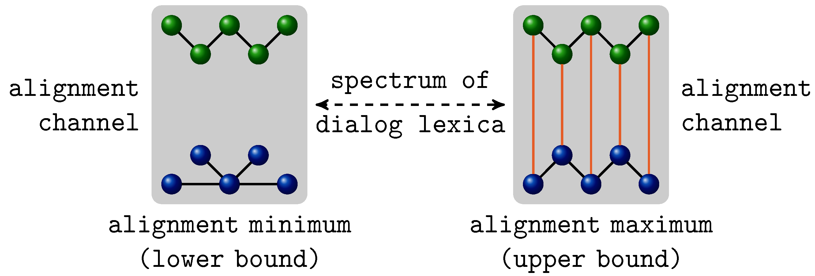
- We develop a framework in which the notion of alignment, that we take to be essential for the understanding of natural language dialog, is operationalized and made measurable. That is, we provide a formal, quantitative model for assessing alignment in dialog.
- This model, and thereby the notion of alignment, is exposed to falsifiability; it is applied to natural language data collected in studies on lexical alignment. Our evaluation indeed yields evidence for alignment in dialog.
- Our framework also implements a developmental model that captures the procedural character of alignment in dialog. Thus, it takes the time-bounded nature of alignment serious and, again, makes it expressible within a formal model and, as a result, measurable.
2. Related Work
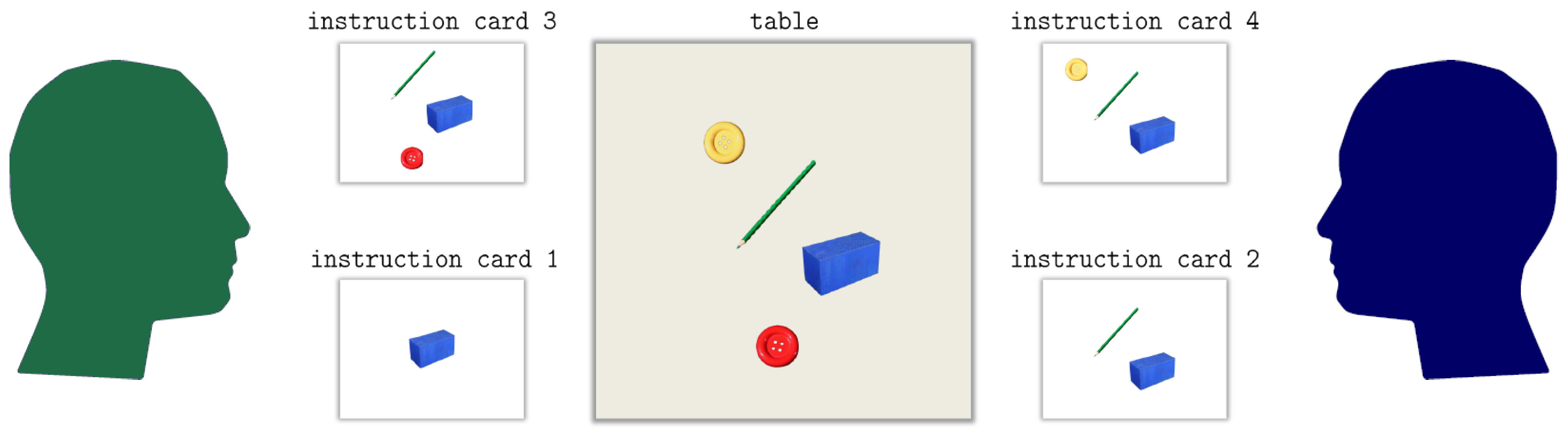
3. An Experimental Setting of Alignment Measurement
4. A Network Model of Alignment in Communication
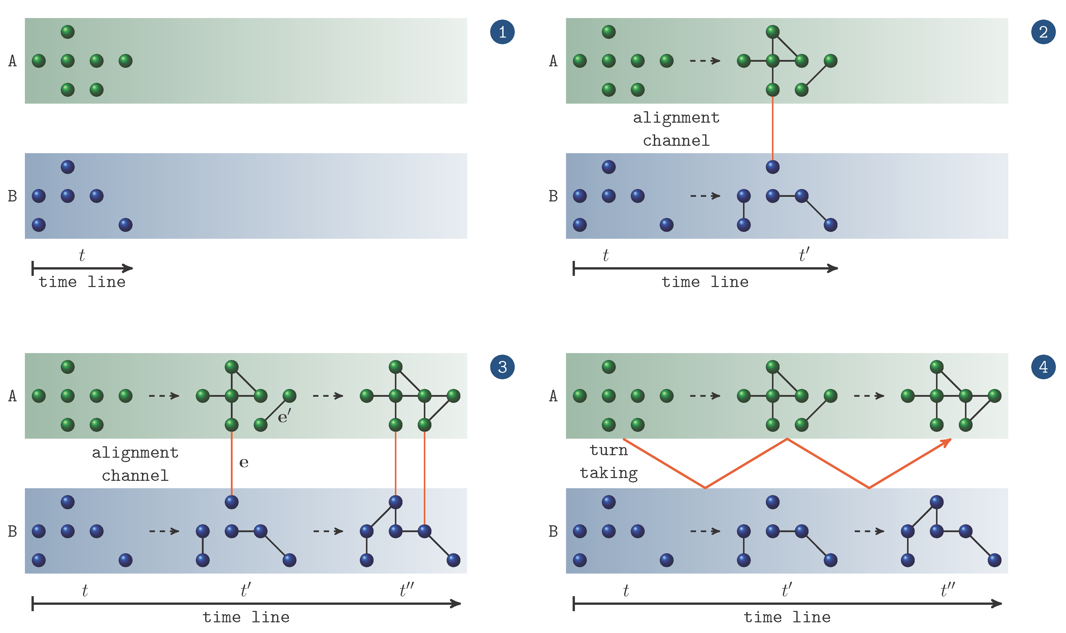
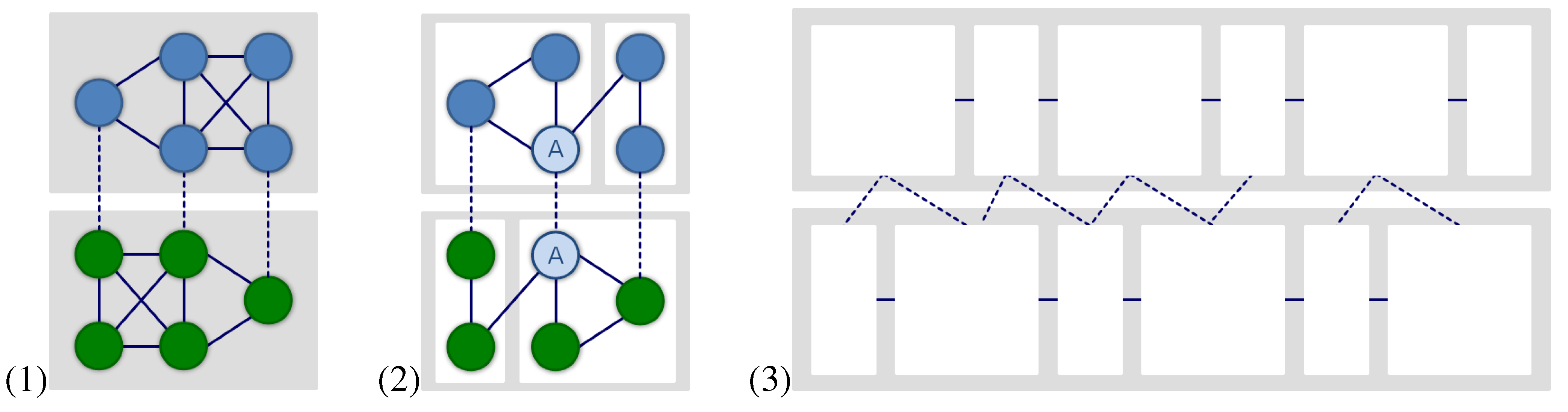
4.1. Two-Layer Time-Aligned Network Series
- Variant I—unlimited memory span:
- −
- Interpersonal links: if at time t, agent uses the item to express the topic that has been expressed by in the same round of the game or in any preceding round on the same topic T by the same item, we span an interpersonal link between and for which , given that e does not already exist. Otherwise, if , its weight is increased by 1. The initial weight of any edge is 1.
- −
- Intrapersonal links: if at time t, agent uses item l to express , we generate intrapersonal links between , , and all other vertices labeled by items that X has used in the same round of the game or in any preceding round on the same topic T. Once more, if the links already exist, their weights are augmented by 1.
Variant I models an unlimited memory where both interlocutors always remember, so to speak, every usage of any item in any preceding round of the game irrespective how long ago it occurred. Obviously, this is an unrealistic scenario that may serve as a borderline case of network induction. A more realistic scenario is given by the following variant that simulates a limited memory. - Variant II—limited memory span:
- −
- Interpersonal links: if at time t, agent uses to express topic that has been expressed by in the same or preceding round on the same topic by the same item, we span an interpersonal link between and for which , given that e does not already exist. Otherwise, e’s weight is adapted as before.
- −
- Intrapersonal links: if at time t, agent uses item l to express , we generate intrapersonal links between , , and all other vertices labeled by items that X has used in the same round or in the preceding round on the same topic T. If the links already exist, their weights are augmented by 1.
4.2. Mutual Information of Two-Layer Networks
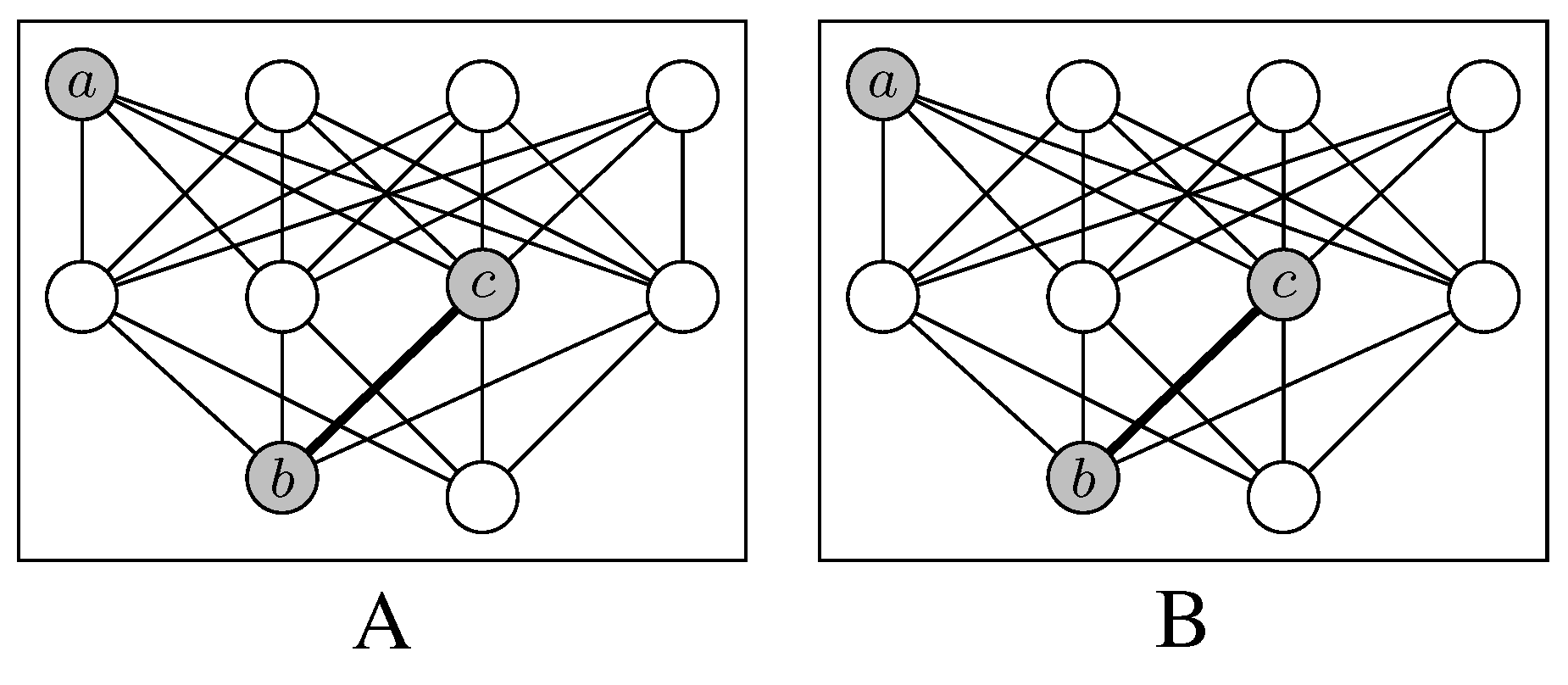
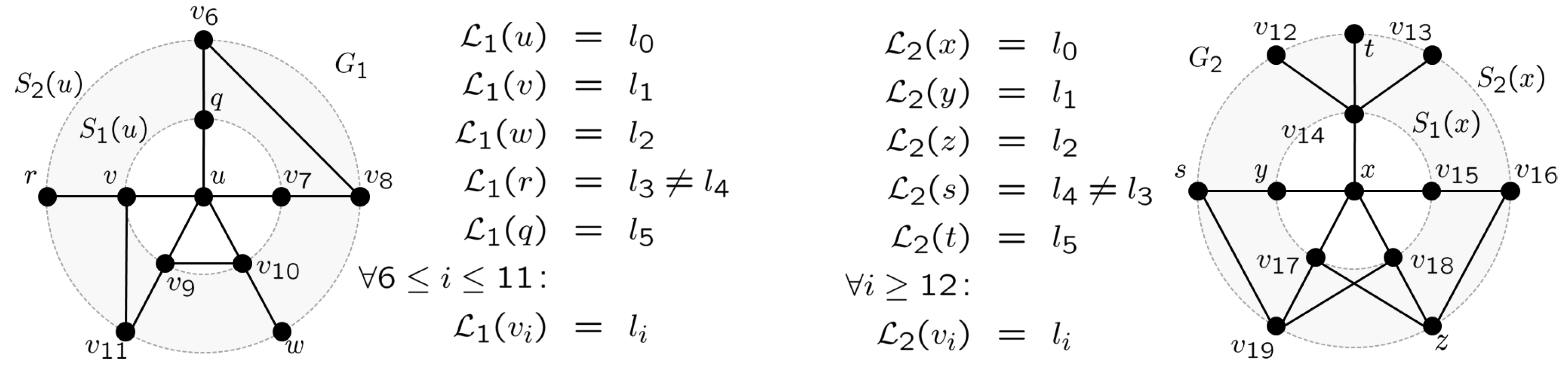
 , that fulfills this condition of unique labeling. In this case, we define for any the j-sphere of v in G as the set: of order | the lexicon of G. The Local Mutual Information (LMI) of the paired primes , , is defined by the quantity
 - ; by definition, paired primes are both located in the zero sphere.
- ; starting from u and x, respectively, is directly associated to in both interlocutor lexica.
- ; exemplifies a word that is mediately associated to their respective primes in both interlocutor lexica the same way.
- is the subset of words in used by speaker A, but not by speaker B.
- is the subset of words in used by speaker A, but not by speaker B.
- is the subset of words in used by speaker B, but not by speaker A.
- is the subset of words in used by speaker B, but not by speaker A.
- ; exemplifies a word that is used by both interlocutors but in a different way from the point of view of the paired primes u and x.
- ; note that 18 = |
![Entropy 12 01440 i001]() | − 1 where
| − 1 where ![Entropy 12 01440 i001]() .
. - .
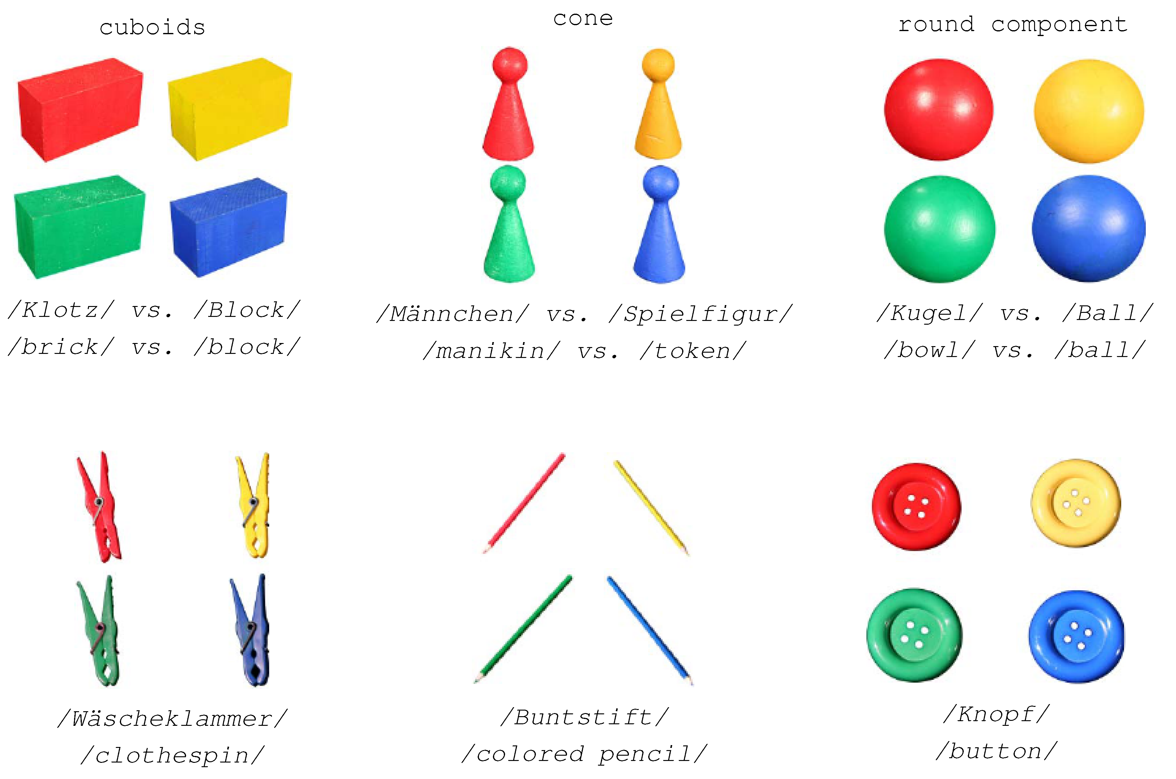
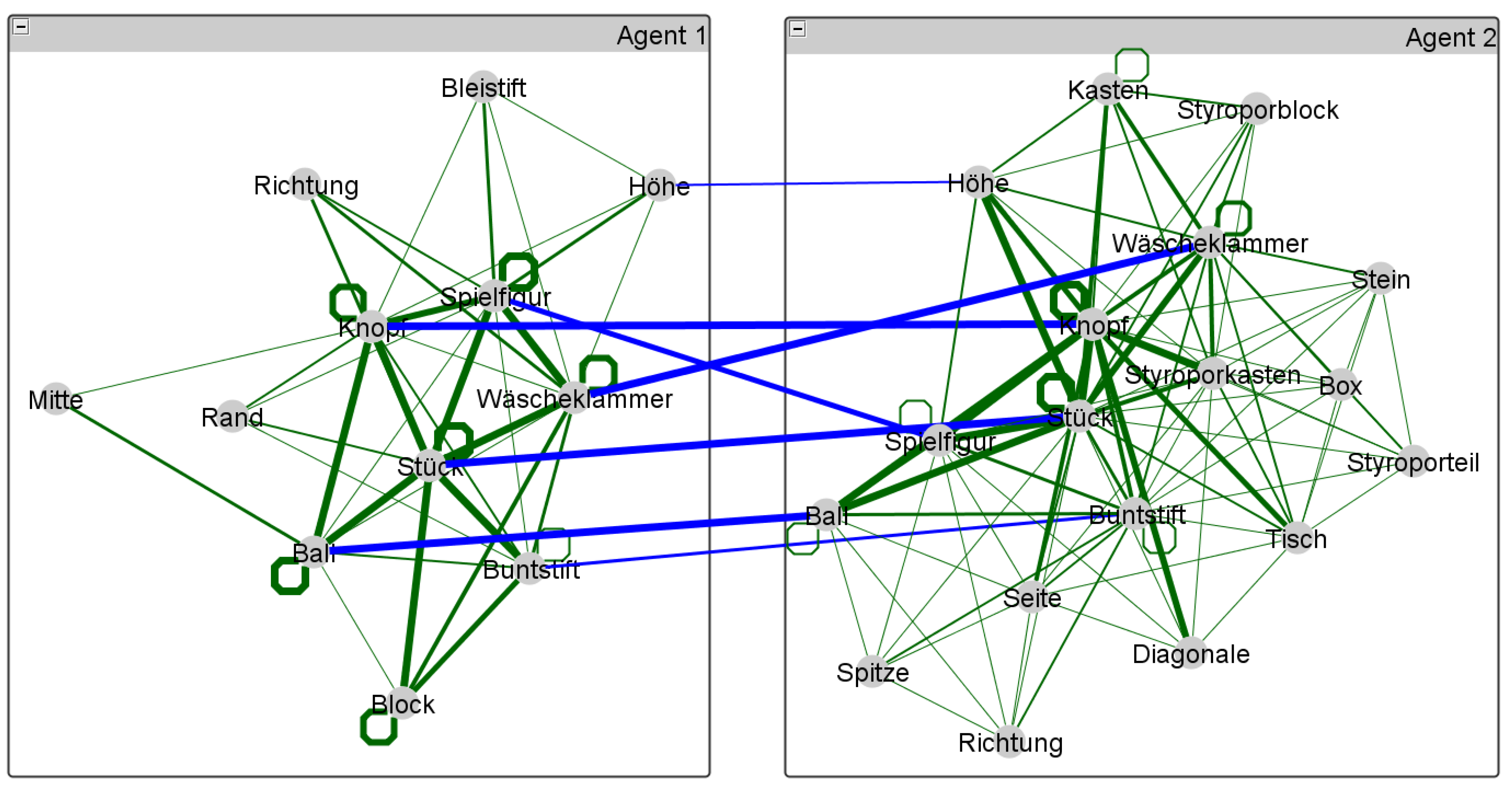
| + 1 to any item in the lexicon of the interlocutor who does not use them.)- On the one hand, both interlocutors are aligned in the sense that they activate a common sub-lexicon during their conversation out of which they recruit paired primes by expressing, for example, the same topic of conversation by the same word. Without such a larger sub-lexicon, the value of could be hardly near to zero as word usages of one interlocutor would tell us nothing about the word usages of the other. Thus, for higher values of it is necessary that the sub-lexicon shared among the interlocutors covers a bigger part of the overall dialog lexicon—note that this notion relates to the notion of graph distance of [59] as explained below. As seen by example of the JMG, there are hardly many paired primes in our study that are common to all pairs of interlocutors. Thus, in order to secure comparability among different pairs of interlocutors, it makes sense to focus on a single lexeme that is actually used by all pairs of interlocutors. In our present study this is exemplified by the lexeme button (see Figure 2 in Section 3).
- On the other hand, both interlocutors are additionally aligned in the sense that the focal primes v and w induce similar patterns of spreading activation [60] within their respective dialog lexica. That is, by commonly using the lexeme that equally labels the vertices v and w, their neighborhoods are activated in a way that is mutually predictable. In terms of geodesic distances, this means that both interlocutors have built dialog lexica that are similarly organized from the point of view of the paired primes v and w.
- First and foremost, we calculate classical indices of complex network theory separately for each of the layers of two-layer networks and aggregate them by a mean value to describe, for example, the average cluster value of interlocutor lexica in dyadic conversations. This is done for the cluster value C1 [61], its weighted correspondents and [62], the normalized average geodesic distance and the closeness centrality of graphs [30,63]. For an undirected graph , is defined as follows:where is the number of vertices in G andpenalizes, so to speak, pairs of unconnected vertices by the theoretical maximum of the diameter of G. measures the proportion of the average geodesic distances of the vertices in relation to the sum of their penalties in the latter sense: the more vertices are connected by the shorter paths, the smaller this proportion such that for completely connected graphs , while for a completely unconnected graph . Computing the normalized variant of the average geodesic distance is indispensable. The reason is that at their beginning, dialog lexica are mainly disconnected so that computing L for their largest connected component would get unrealistically small values.
- The latter group of indices simply adapts classical notions of complex network theory to the area of two-layer networks. That is, they do not measure the dissimilarity of graphs as done, for example, by . As an alternative to D, we utilize two graph distance measures [64,65,66]. More specifically, [59] consider the following quantity to measure the distance of two (labeled) graphs :where is the maximum common subgraph of and and is the order of . This measure has very interesting properties: firstly, if and are uniquely labeled and if the computation of reflects this labeling, it is efficiently computable. Further is a metric and, thus, computes easily interpretable graph distances [60]. In this line of research, [67] propose a graph distance measure based on graph union:Both of these measures compute graph distances and are therefore applicable to measuring the dissimilarity of dialog lexica distributed among interlocutors. Consequently, we apply them in addition to D and S, respectively, to extend our tertium comparationis.
- Last but not least, we consider an index of modularity that, for a given network, measures the independence of its candidate modules. As we consider networks with two modules, we use the following variant of the index of [68]:where is the number of links within the ith part of the network and is the number of links across the alignment channel.
5. Random Models of Two-Layer Networks
| Algorithm 1: Binomial case I: computing a set of randomized TiTAN series. |
| Data: TiTAN series ; number of iterations n Result: Set of n randomized TiTAN series for do rewire at random to get ; for do randomly delete edges from to get ; ; end ; ; end |
| Algorithm 2: Binomial case II: computing a set of layer-sensitive randomized TiTAN series. |
| Data: TiTAN series ; number of iterations n Result: Set of n randomized TiTAN series for do rewire , and at random to build where such that , and ; for do randomly delete edges from to get ; randomly delete edges from to get ; randomly delete edges from to get ; set such that and , and ; end ; ; end |
5.1. The Binomial Model (BM-I)
5.2. The Partition-Sensitive Binomial Model (BM-II)
5.3. The Partition- and Edge-Identity-Sensitive Binomial Model (BM-III)
5.4. The Event-Related Shuffle Model (SM-I)
5.5. The Time Point-Related Shuffle Model (SM-II)
5.6. Summary Attributes of Randomized Two-Layer Networks
6. Experimentation
6.1. On the Temporal Dynamics of Lexical Alignment
Lexical Clustering
Lexical Closeness
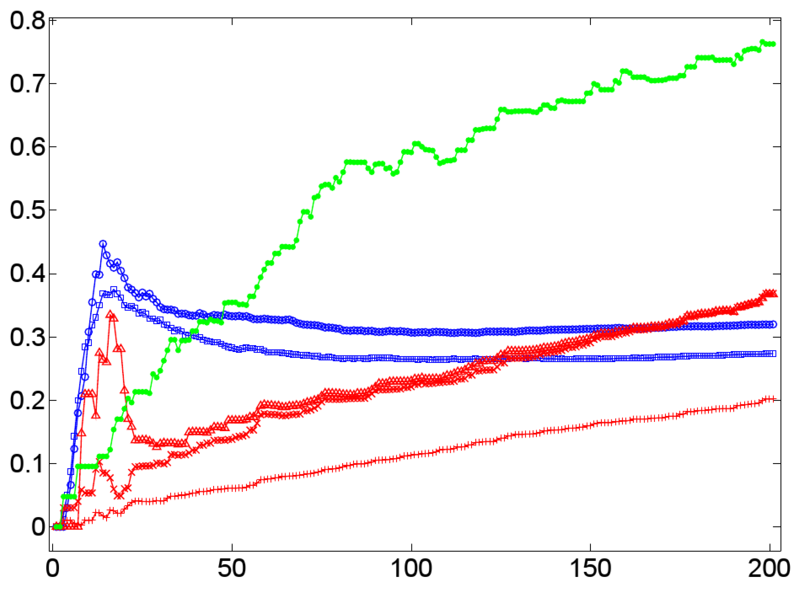
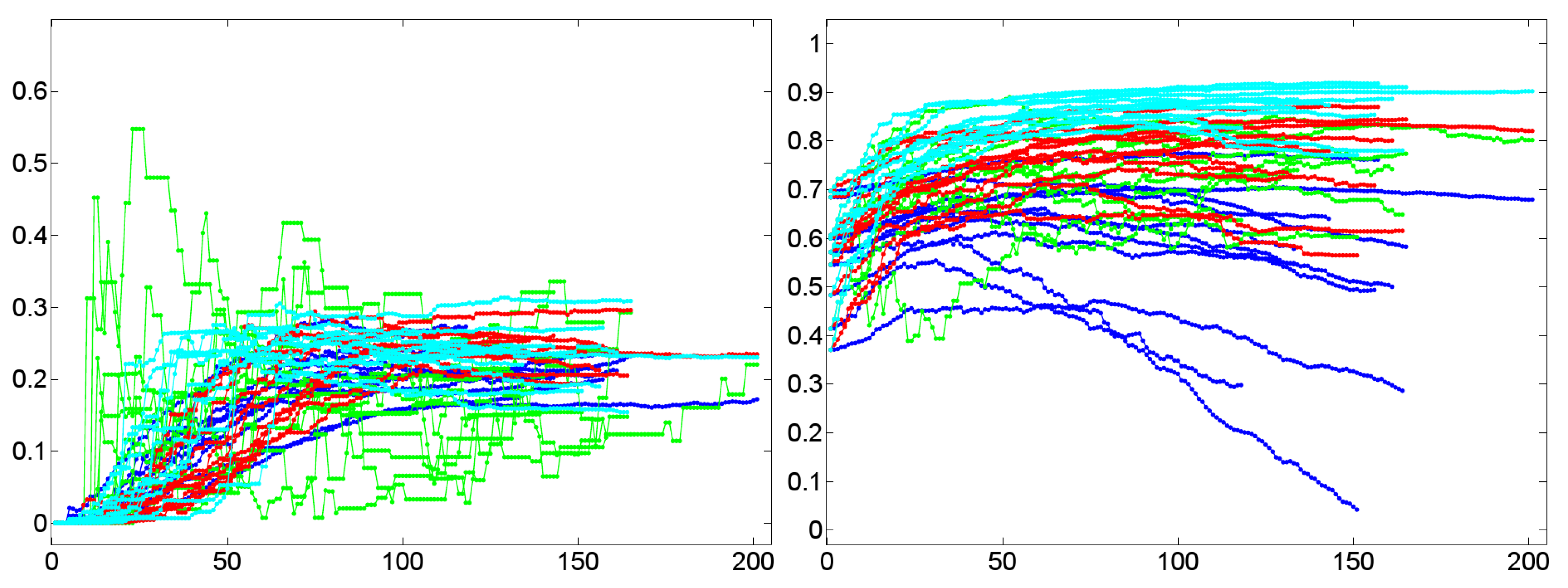
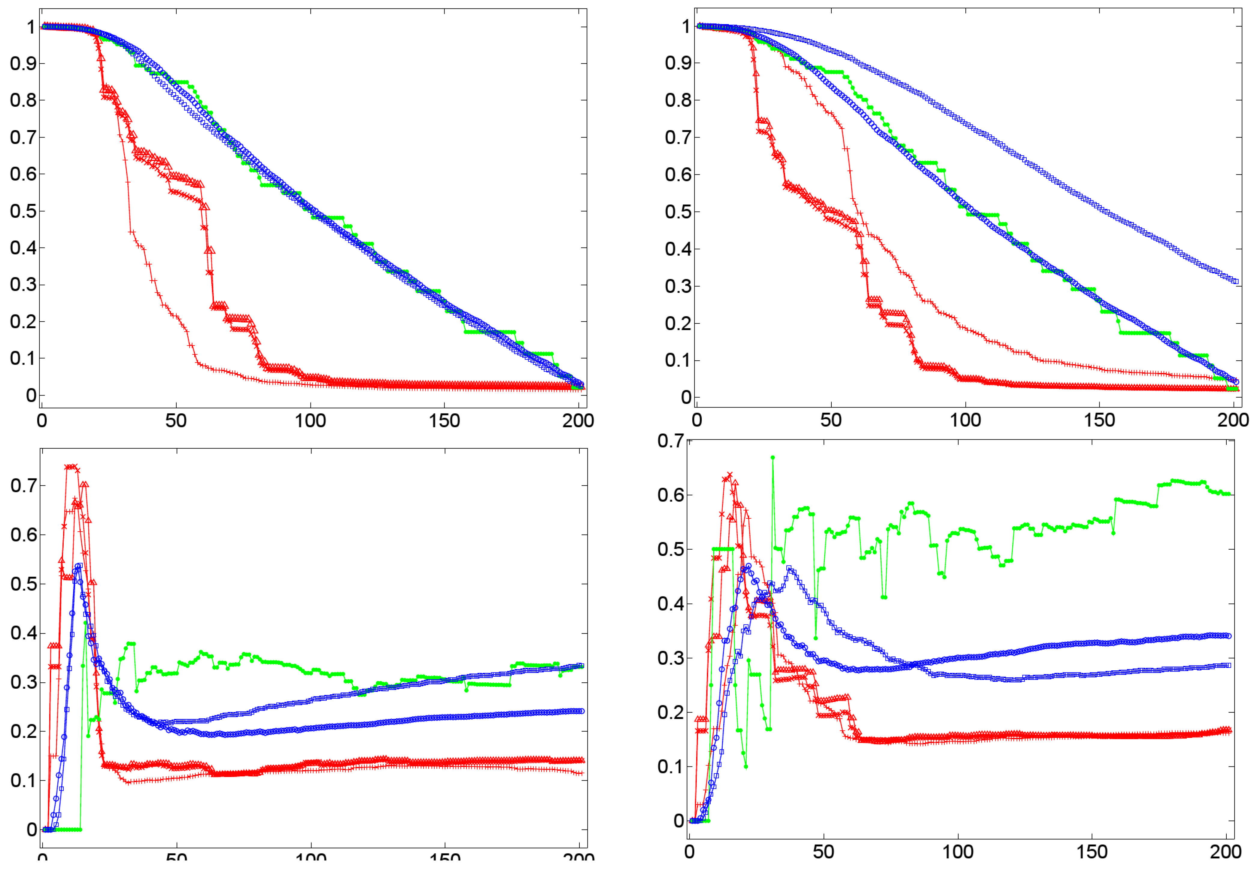
- A low value of for a graph G indicates short paths between any pair of vertices in G that tends to be connected without any two disconnected components. In terms of dialog lexica this is tantamount to a high probability that any prime may activate any other item in the lexicon even though to a low degree. In other words, when receiving a word form /a/, the dialog lexicon of an interlocutor allows, in principle, for activating the complete sublexicon that he has generated till the moment of processing /a/. Both of these assessments are confirmed by our corpus of 11 experimental dialogs. The upper left part of Figure 12 reports the temporal dynamics of in Dialog 19, while the upper right part of Figure 12 depicts the values of after being averaged over both interlocutor lexica. In both cases, we observe that short average geodesic distances emerge much more rapidly in the BM-I, the BM-II, and the BM-III. We also observe that all variants (whether natural or randomized) result in very low values of indicating the existence of the latter mechanism. However, we also observe that the SM-II (based on shuffling the time points of dialog events) perfectly approximates geodesic distances in natural dialogs. In any event, as dialog lexica finally produce short average geodesic distances, even though more slower than their binomial counterparts, they perfectly fit into the class of networks that have been called small-worlds ([61,73]) as they also have high cluster values. Note that the upper left and right part of Figure 12 hints at a constant drop of as the dialog evolves. In other words, nouns as considered here are not distinguished in their contribution to the decrease of as a function of the time of their utterance. This may explain why the SM-II approximates the dynamics of in natural dialogs.
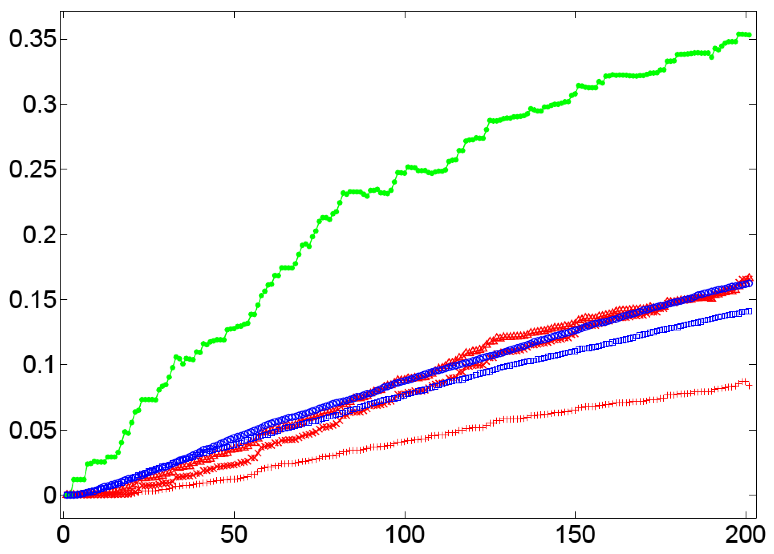
- A high closeness centrality of a graph G indicates that its vertices coincide more or less regarding the sum of their geodesic distances to all other vertices of G [30]. In conjunction with a value of near to zero this means that all vertices operate on an equal footing as efficient entry points to the lexicon by which any other item is accessible with almost the same effort of spreading activation. This picture is only confirmed, if we average the standardized closeness centrality over both interlocutor lexica (depicted by the lower right part of Figure 12). Obviously, Dialog 19 has a much higher closeness centrality than its random counterparts.
Lexical Modularity
Lexical Similarity
6.2. A Classification Model of Alignment
- In spite of the fact that annotating dialogical data is very effortful so that even 24 dialogs can be seen to be a data set of medium size, any classification result based on such a small set is hardly expressive.
- On the other hand, alignment is a process variable that does not (necessarily) emerge suddenly at the endpoint of a conversation. Rather, alignment gradually evolves so that it is present at different stages of a conversation by different, possibly non-monotonic degrees. According to this view, we need to evaluate a larger interval of a conversation when measuring its alignment—ideally beginning with its end in a regressive manner.
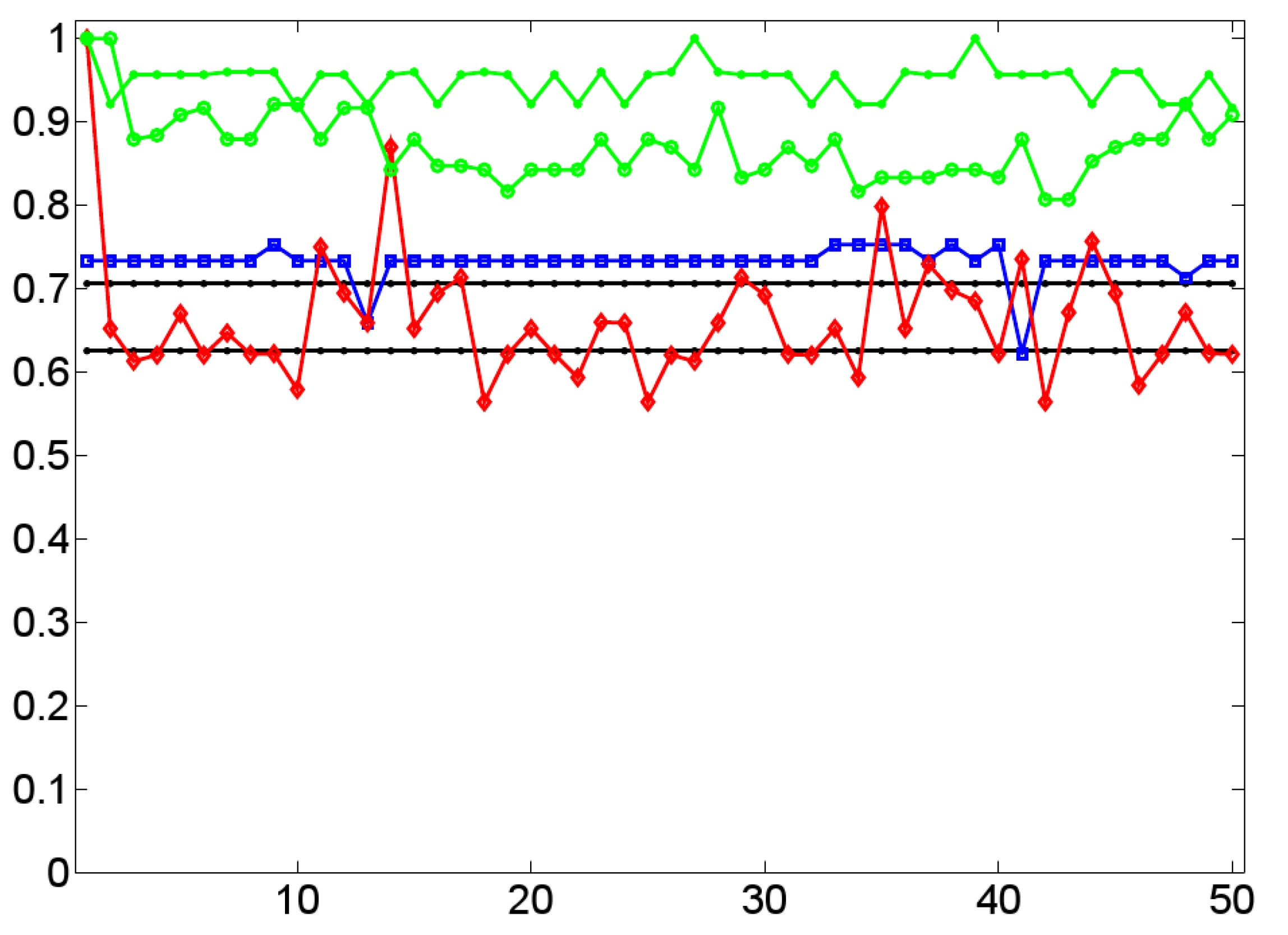
- Straight lines parallel to the x-axis denote the F-scores of two baselines: (i) the known-partition-scenario (with an F-score of ) that has knowledge about the cardinality of each target class, and (ii) the equi-partition-scenario (with an F-score of ) that assumes equally sized target classes. Computing these baselines is done 1,000 times so that Figure 16 shows their average F-scores. Roughly speaking, an F-score of means that about 70% of dialogs are correctly classified by randomly assigning them onto both target classes subject to knowing their cardinality—a remarkably high value.
- On the opposite range of the curves in Figure 16 we get the values of the best performing classification (denoted by bullets). In each of the 50 classifications, reported by Figure 16, this variant integrates a genetic search for the best performing subset of 50 topological features. This includes indices of complex network theory (as, for example, the cluster coefficient and the average geodesic distance [73]), graph centrality measures [63], entropy measures ([52,75]) as well as the graph similarity measures described in Section 4.2. According to Figure 16, this variant produces a maximal F-score of in the case of three different classifications—this holds especially for the endpoint of the time series under consideration (with the x-coordinate 1). On average, this variant reaches an F-score of . That is, nearly percent of the dialogs are correctly classified by this nearly optimal approach. Thus, using a wide range of topological indices together with an optimization algorithm seems to perform very well, but to the price of an optimization that runs the risk of overfitting.
- In order to shed light on this risk, we compute two additional alternatives. Firstly, Figure 16 shows the values of a genetic search (denoted by circles) on the subset of those 12 features that result in an F-score of for the dialogs’ endpoints. We observe a loss in F-score down to an average score of , which, at first glance, does not seem to be dramatic. But things are different if we apply the same subset of features in each of the fifty classifications without any additional optimization. In this case, the average F-score drops down to (i.e., below the upper baseline). Obviously, the optimized classifier performs very unreliably. That is, although we can classify two-layer networks according to (non-)alignment, the classifiers considered so far should be treated very carefully when processing heretofore unseen data.
- Figure 16 also shows that the latter assessment is preliminary. It presents the F-scores of a variant (denoted by squares) that has been produced by two features only, that is, (using the lexeme button as the single paired prime) and . On the one hand, we see that this variant produces an average F-score of only and, thus, outperforms the upper-bound of both baselines on a rather low level. Further, it also generates two outliers that fall below this upper-bound. However, we also observe that this variant produces very stable results by means of only two indices that according to Section 16, directly relate to alignment measurement. Moreover, the outlier on the right side of the corresponding curve may be due to a loss in the prominence of alignment at this earlier stage of conversation.
7. General Discussion
8. Conclusions
Acknowledgement
References
- Pickering, M.J.; Garrod, S. Toward a mechanistic psychology of dialogue. Behav. Brain. Sci. 2004, 27, 169–226. [Google Scholar] [CrossRef] [PubMed]
- Clark, H.H. Using Language; Cambridge University Press: Cambridge, UK, 1996. [Google Scholar]
- Maturana, H.R.; Varela, F.J. Autopoiesis and Cognition. The Realization of the Living; Reidel: Dordrecht, The Netherlands, 1980. [Google Scholar]
- Levelt, W.J.M. Speaking. From Intention to Articulation; MIT Press: Cambridge, MA, USA, 1989. [Google Scholar]
- Giles, H.; Powesland, P.F. Speech Styles and Social Evaluation; Academic Press: London, UK / New York, NY, USA, 1975. [Google Scholar]
- Clark, H.H.; Wilkes-Gibbs, D. Referring as a collaborative process. Cognition 1986, 22, 1–39. [Google Scholar] [CrossRef]
- Branigan, H.P.; Pickering, M.J.; Cleland, A.A. Syntactic coordination in dialogue. Cognition 2000, 25, B13–B25. [Google Scholar] [CrossRef]
- Garrod, S.; Anderson, A. Saying what you mean in dialogue: a study in conceptual and semantic co-ordination. Cognition 1987, 27, 181–218. [Google Scholar] [CrossRef]
- Watson, M.E.; Pickering, M.J.; Branigan, H.P. An empirical investigation into spatial reference frame taxonomy using dialogue. In Proceedings of the 26th Annual Conference of the Cognitive Science Society, Chicago, IL, USA, 2004; pp. 2353–2358.
- Kamp, H.; Reyle, U. From Discourse to Logic. Introduction to Modelltheoretic Semantics of Natural Language, Formal Logic and Discourse Representation Theory; Kluwer: Dordrecht, The Netherlands, 1993. [Google Scholar]
- Lewis, D. Conventions. A Philosophical Study; Harvard University Press: Cambridge, MA, USA, 1969. [Google Scholar]
- Stalnaker, R. Common ground. Linguist. Phil. 2002, 25, 701–721. [Google Scholar] [CrossRef]
- Collins, A.M.; Loftus, E.F. A spreading-activation theory of semantic processing. Psychol. Rev. 1975, 82, 407–428. [Google Scholar] [CrossRef]
- Kopp, S.; Rieser, H.; Wachsmuth, I.; Bergmann, K.; Lücking, A. Speech-Gesture alignment. In Project Panel at the 3rd International Conference of the International Society for Gesture Studies, Evanston, IL, USA, June, 2007.
- Lücking, A.; Mehler, A.; Menke, P. Taking fingerprints of speech-and-gesture ensembles: approaching empirical evidence of intrapersonal alignment in multimodal communication. In Proceedings of the 12th Workshop on the Semantics and Pragmatics of Dialogue, King’s College, London, UK, June 2008; pp. 157–164.
- Church, K.W. Empirical estimates of adaptation: the chance of two noriegas is closer to p/2 than p2. In Proceedings of Coling 2000, Saarbrücken, Germany, July-August 2000; pp. 180–186.
- Reitter, D.; Keller, F.; Moore, J.D. Computational modelling of structural priming in dialogue. In Proceedings of the Human Language Technology Conference of the North American Chapter of the Association for Computational Linguistics, New York, NY, USA, June 2006; pp. 121–124.
- Wheatley, B.; Doddington, G.; Hemphill, C.; Godfrey, J.; Holliman, E.; McDaniel, J.; Fisher, D. Robust automatic time alignment of orthographic transcriptions with unconstrained speech. In Proceedings of IEEE International Conference on Acoustics, Speechand Signal Processing (ICASSP-92), San Francisco, CA, USA, March 1992; pp. 533–536.
- Anderson, A.H.; Bader, M.; Gurman Bard, E.; Boyle, E.; Doherty, G.; Garrod, S. The HCRC map task corpus. Lang. Speech 1991, 34, 351–366. [Google Scholar]
- Reitter, D.; Moore, J.K. Predicting success in dialogue. In Proceedings of the 45th Annual Meeting of the Association of Computational Linguistics (ACL), Praque, Czech Republic, June 2007; pp. 808–815.
- Branigan, H.P.; Pickering, M.J.; McLean, J.F.; Cleland, A.A. Syntactic alignment and participant role in dialogue. Cognition 2007, 104, 163–197. [Google Scholar] [CrossRef] [PubMed]
- Garrod, S.; Fay, N.; Lee, J.; Oberlander, J.; MacLeod, T. Foundations of representations: where might graphical symbol systems come from? Cogn. Sci. 2007, 31, 961–987. [Google Scholar] [CrossRef] [PubMed]
- Fay, N.; Garrod, S.; Roberts, L. The fitness and functionality of culturally evolved communication systems. Philos. Trans. R. Soc. Lond. B Biol. Sci. 2008, 363, 3553–3561. [Google Scholar] [CrossRef] [PubMed]
- Schober, M.F.; Brennan, S.E. Processes of interactive spoken discourse: the role of the partner. In Handbook of Discourse Processes; Erlbaum: Mahwah, NJ, USA, 2003. [Google Scholar]
- Krauss, R.M.; Weinheimer, S. Concurrent feedback, confirmation, and the encoding of referents in verbal communication. J. Pers. Soc. Psychol. 1966, 4, 343–346. [Google Scholar] [CrossRef] [PubMed]
- Weiß, P.; Pfeiffer, T.; Schaffranietz, G.; Rickheit, G. Coordination in dialog: alignment of object naming in the Jigsaw Map Game. In Proceedings of the 8th Annual Conference of the Cognitive Science Society of Germany, Saarbrücken, Germany, August 2007; pp. 4–20.
- Gleim, R.; Mehler, A.; Eikmeyer, H.J. Representing and maintaining large corpora. In Proceedings of the Corpus Linguistics 2007 Conference, Birmingham, UK, July 2007.
- Ferrer i Cancho, R.; Solé, R.V. The small-world of human language. Proc. R. Soc. Lond. B Biol. Sci. 2001, 268, 2261–2265. [Google Scholar] [CrossRef] [PubMed]
- Ferrer i Cancho, R.; Solé, R.V.; Köhler, R. Patterns in syntactic dependency-networks. Phys. Rev. E 2004, 69, 051915. [Google Scholar] [CrossRef] [PubMed]
- Mehler, A. Structural similarities of complex networks: a computational model by example of Wiki graphs. Appl. Artif. Intell. 2008, 22, 619–683. [Google Scholar] [CrossRef]
- Mehler, A. On the impact of community structure on self-organizing lexical networks. In Proceedings of the 7th Evolution of Language Conference (Evolang7), Barcelona, Spain, March 2008; pp. 227–234.
- Motter, A.E.; de Moura, A.P.S.; Lai, Y.C.; Dasgupta, P. Topology of the conceptual network of language. Phys. Rev. E 2002, 65. [Google Scholar] [CrossRef] [PubMed]
- Mukherjee, A.; Choudhury, M.; Basu, A.; Ganguly, N. Self-organization of the sound inventories: analysis and synthesis of the occurrence and co-occurrence networks of consonants. J. Quant. Linguist. 2009, 16, 157–184. [Google Scholar] [CrossRef]
- Steyvers, M.; Tenenbaum, J. The large-scale structure of semantic networks: Statistical analyses and a model of semantic growth. Cogn. Sci. 2005, 29, 41–78. [Google Scholar] [CrossRef] [PubMed]
- Church, K.W.; Hanks, P. Word association norms, mutual information, and lexicography. Comput. Linguist. 1990, 16, 22–29. [Google Scholar]
- Miller, G.A.; Charles, W.G. Contextual correlates of semantic similarity. Lang. Cogn. Process 1991, 6, 1–28. [Google Scholar] [CrossRef]
- Mehler, A. Large text networks as an object of corpus linguistic studies. In Corpus Linguistics. An International Handbook of the Science of Language and Society; De Gruyter: Berlin, Germany/New York, NY, USA, 2008; pp. 328–382. [Google Scholar]
- Diestel, R. Graph Theory; Springer: Heidelberg, Germany, 2005. [Google Scholar]
- Branigan, H.P.; Pickering, M.J.; Cleland, A.A. Syntactic priming in written production: evidence for rapid decay. Psychon. Bull. Rev. 1999, 6, 635–640. [Google Scholar] [CrossRef] [PubMed]
- Bock, K.; Griffin, Z.M. The persistence of structural priming: transient activation or implicit learning? J. Exp. Psychol. 2000, 129, 177–192. [Google Scholar] [CrossRef]
- Ferreira, V.S.; Bock, K. The functions of structural priming. Lang. Cogn. Process 2006, 21, 1011–1029. [Google Scholar] [CrossRef] [PubMed]
- Mehler, A.; Weiß, P.; Menke, P.; Lücking, A. Towards a simulation model of dialogical alignment. In Proceedings of the 8th International Conference on the Evolution of Language (Evolang8), Utrecht, The Netherlands, April 2010.
- Halliday, M.A.K. Lexis as a linguistic level. In In Memory of J. R. Firth; Longman: London, UK, 1966. [Google Scholar]
- Rieger, B.B. Semiotic cognitive information processing: learning to understand discourse. A systemic model of meaning constitution. In Adaptivity and Learning. An Interdisciplinary Debate; Springer: Berlin, Germany, 2003; pp. 347–403. [Google Scholar]
- Barrat, A.; Barthélemy, M.; Vespignani, A. Dynamical Processes on Complex Networks; Cambridge University Press: Cambridge, UK, 2008. [Google Scholar]
- Caldarelli, G. Scale-Free Networks. Complex Webs in Nature and Technology; Oxford Uiversity Press: Oxford, UK, 2008. [Google Scholar]
- Caldarelli, G.; Vespignani, A. Large Scale Structure and Dynamics of Complex Networks; World Scientific: Hackensack, NJ, USA, 2007. [Google Scholar]
- Pastor-Satorras, R.; Vespignani, A. Evolution and Structure of the Internet; Cambridge University Press: Cambridge, UK, 2004. [Google Scholar]
- Bunke, H. What is the distance between graphs? Bull. EATCS 1983, 20, 35–39. [Google Scholar]
- Garey, M.R.; Johnson, D.S. Computers and Intractability: A Guide to the Theory of NP-Completeness; W.H. Freeman: New York, NY, USA, 1979. [Google Scholar]
- Wilhelm, T.; Hollunder, J. Information theoretic description of networks. Phys. A 2007, 385. [Google Scholar] [CrossRef]
- Dehmer, M. Information processing in complex networks: graph entropy and information functionals. Appl. Math. Comput. 2008, 201, 82–94. [Google Scholar] [CrossRef]
- Bonchev, D. Information Theoretic Indices for Characterization of Chemical Structures; Research Studies Press: Chichester, UK, 1983. [Google Scholar]
- Kraskov, A.; Grassberger, P. MIC: mutual information based hierarchical clustering. In Information Theory and Statistical Learning; Springer: New York, NY, USA, 2008; pp. 101–123. [Google Scholar]
- Dehmer, M.; Varmuza, K.; Borgert, S.; Emmert-Streib, F. On entropy-based molecular descriptors: statistical analysis of real and synthetic chemical structures. J. Chem. Inf. Model. 2009, 49, 1655–1663. [Google Scholar] [CrossRef] [PubMed]
- Dehmer, M.; Barbarini, N.; Varmuza, K.; Graber, A. A large scale analysis of information-theoretic network complexity measures using chemical structures. PLoS One 2009, 4, e8057. [Google Scholar] [CrossRef] [PubMed]
- Tuldava, J. Methods in Quantitative Linguistics; Wissenschaftlicher Verlag: Trier, Germany, 1995. [Google Scholar]
- Cover, T.M.; Thomas, J.A. Elements of Information Theory; Wiley-Interscience: Hoboken, NY, USA, 2006. [Google Scholar]
- Bunke, H.; Shearer, K. A graph distance metric based on the maximal common subgraph. Pattern Recogn. Lett. 1998, 19, 255–259. [Google Scholar] [CrossRef]
- Gärdenfors, P. Conceptual Spaces; MIT Press: Cambridge, MA, USA, 2000. [Google Scholar]
- Watts, D.J.; Strogatz, S.H. Collective dynamics of `small-world’ networks. Nature 1998, 393, 440–442. [Google Scholar] [CrossRef] [PubMed]
- Serrano, M.Á.; Boguñá, M.; Pastor-Satorras, R. Correlations in weighted networks. Phys. Rev. E 2006, 74, 055101. [Google Scholar] [CrossRef] [PubMed]
- Feldman, R.; Sanger, J. The Text Mining Handbook. Advanced Approaches in Analyzing Unstructured Data; Cambridge University Press: Cambridge, UK, 2007. [Google Scholar]
- Bunke, H.; Günter, S. Weighted mean of a pair of graphs. Computing 2001, 67, 209–224. [Google Scholar] [CrossRef]
- Bunke, H.; Günter, S.; Jiang, X. Towards bridging the gap between statistical and structural pattern recognition: two new concepts in graph matching. In Proceedings of the Second International Conference on Advances in Pattern Recognition; Springer: Berlin, Germany/New York, NY, USA, 2001; pp. 1–11. [Google Scholar]
- Schenker, A.; Bunke, H.; Last, M.; Kandel, A. Graph-Theoretic Techniques for Web Content Mining; World Scientific: Hackensack, NJ, USA/London, UK, 2005. [Google Scholar]
- Wallis, W.D.; Shoubridge, P.; Kraetz, M.; Ray, D. Graph distances using graph union. Pattern Recogn. Lett. 2001, 22, 701–704. [Google Scholar] [CrossRef]
- Newman, M.E.J.; Girvan, M. Finding and evaluating community structure in networks. Phys. Rev. E 2004, 69, 026113. [Google Scholar] [CrossRef] [PubMed]
- Erdős, P.; Rényi, A. On random graphs. Publ. Math. 1959, 6, 290–297. [Google Scholar]
- Cattuto, C.; Barrat, A.; Baldassarri, A.; Schehr, G.; Loreto, V. Collective dynamics of social annotation. PNAS 2009, 106, 10511–10515. [Google Scholar] [CrossRef] [PubMed]
- Zlatic, V.; Bozicevic, M.; Stefancic, H.; Domazet, M. Wikipedias: Collaborative web-based encyclopedias as complex networks. Phys. Rev. E 2006, 74, 016115. [Google Scholar] [CrossRef] [PubMed]
- Mehler, A. Text linkage in the Wiki medium — a comparative study. In Proceedings of the EACL Workshop on New Text — Wikis and blogs and other dynamic text sources, Trento, Italy, April 2006; pp. 1–8.
- Newman, M.E.J. The structure and function of complex networks. SIAM Rev. 2003, 45, 167–256. [Google Scholar] [CrossRef]
- Altmann, G. Semantische diversifikation. Folia Linguist. 1985, 19, 177–200. [Google Scholar] [CrossRef]
- Mehler, A. A quantitative graph model of social ontologies by example of Wikipedia. In Towards an Information Theory of Complex Networks: Statistical Methods and Applications; Birkhäuser: Boston, MA, USA/Basel, Switzerland, 2009. [Google Scholar]
- Manning, C.D.; Schütze, H. Foundations of Statistical Natural Language Processing; MIT Press: Cambridge, MA, USA, 1999. [Google Scholar]


| Network | Alignment | #events | #turns | ||||
| 1 | no | 39 | 197 | 15 | 24 | 123 | 30 |
| 1 | yes | 44 | 267 | 25 | 19 | 164 | 36 |
| 4 | yes | 34 | 145 | 15 | 19 | 100 | 30 |
| 5 | no | 39 | 232 | 17 | 22 | 118 | 34 |
| 5 | yes | 42 | 254 | 23 | 19 | 143 | 31 |
| 6 | no | 43 | 227 | 21 | 22 | 113 | 30 |
| 6 | yes | 46 | 343 | 23 | 23 | 151 | 34 |
| 7 | yes | 37 | 145 | 17 | 20 | 111 | 36 |
| 7 | no | 43 | 227 | 20 | 23 | 165 | 30 |
| 8 | yes | 39 | 163 | 18 | 21 | 112 | 30 |
| 8 | yes | 46 | 237 | 18 | 28 | 161 | 52 |
| 19 | yes | 40 | 169 | 18 | 22 | 110 | 32 |
| 19 | yes | 63 | 367 | 28 | 35 | 201 | 48 |
| 33 | yes | 27 | 104 | 12 | 15 | 96 | 32 |
| 33 | yes | 44 | 225 | 18 | 26 | 156 | 50 |
| 34 | no | 34 | 137 | 13 | 21 | 117 | 34 |
| 34 | yes | 32 | 146 | 17 | 15 | 118 | 28 |
| 35 | yes | 20 | 65 | 9 | 11 | 100 | 30 |
| 36 | yes | 37 | 133 | 13 | 24 | 113 | 41 |
| 36 | yes | 50 | 213 | 30 | 20 | 134 | 42 |
| 37 | yes | 24 | 111 | 11 | 13 | 98 | 34 |
| 37 | yes | 40 | 216 | 20 | 20 | 133 | 30 |
| 38 | yes | 30 | 140 | 12 | 18 | 118 | 28 |
| 38 | yes | 50 | 244 | 31 | 19 | 157 | 41 |
© 2010 by the authors; licensee MDPI, Basel, Switzerland. This article is an Open Access article distributed under the terms and conditions of the Creative Commons Attribution license http://creativecommons.org/licenses/by/3.0/.
Share and Cite
Mehler, A.; Lücking, A.; Weiß, P. A Network Model of Interpersonal Alignment in Dialog. Entropy 2010, 12, 1440-1483. https://doi.org/10.3390/e12061440
Mehler A, Lücking A, Weiß P. A Network Model of Interpersonal Alignment in Dialog. Entropy. 2010; 12(6):1440-1483. https://doi.org/10.3390/e12061440
Chicago/Turabian StyleMehler, Alexander, Andy Lücking, and Petra Weiß. 2010. "A Network Model of Interpersonal Alignment in Dialog" Entropy 12, no. 6: 1440-1483. https://doi.org/10.3390/e12061440