Entropy Generation Analysis of Desalination Technologies

Abstract

Increasing global demand for fresh water is driving the development and implementation of a wide variety of seawater desalination technologies. Entropy generation analysis, and specifically, Second Law efficiency, is an important tool for illustrating the influence of irreversibilities within a system on the required energy input. When defining Second Law efficiency, the useful exergy output of the system must be properly defined. For desalination systems, this is the minimum least work of separation required to extract a unit of water from a feed stream of a given salinity. In order to evaluate the Second Law efficiency, entropy generation mechanisms present in a wide range of desalination processes are analyzed. In particular, entropy generated in the run down to equilibrium of discharge streams must be considered. Physical models are applied to estimate the magnitude of entropy generation by component and individual processes. These formulations are applied to calculate the total entropy generation in several desalination systems including multiple effect distillation, multistage flash, membrane distillation, mechanical vapor compression, reverse osmosis, and humidification-dehumidification. Within each technology, the relative importance of each source of entropy generation is discussed in order to determine which should be the target of entropy generation minimization. As given here, the correct application of Second Law efficiency shows which systems operate closest to the reversible limit and helps to indicate which systems have the greatest potential for improvement.

1. Introduction

Water demand is growing worldwide as a result of rising population, increasing standards of living, industrialization, and, in some instances, wasteful water use and management policies. Substantial water shortages and scarcity have appeared. Although developing countries are often hardest hit, water scarcity is a very real problem for developed countries as well [1,2]. Various seawater desalination technologies have been developed in order to try to introduce new sources of water in an attempt to meet growing water needs [3,4].

Advances over the last several decades have dramatically reduced the energy costs associated with seawater desalination. However, seawater desalination is still an energy intensive process that is made more so as a result of irreversibilities within the various system components. Therefore, there is a need to understand and reduce the sources of irreversibility within the systems in order to improve their performance and reduce energy consumption. In order to gain a deeper understanding of the irreversibilities, a Second Law analysis is used to determine the components with maximum entropy generation in six different systems: multiple effect distillation (MED), multistage flash (MSF), direct contact membrane distillation (DCMD), mechanical vapor compression (MVC), reverse osmosis (RO), and humidification-dehumidification (HD or HDH).

Second Law analysis of desalination systems is not new [5,6,7,8,9,10,11]. However, there have been many conflicting definitions for Second Law efficiency; and, to the authors’ knowledge, comprehensive studies identifying all sources of entropy generation have not been conducted. In this paper, a consistent definition of Second Law efficiency for desalination systems based on the least work of separation is presented. Additionally, the required work of separation is decomposed into the least work of separation plus the contribution from all significant sources of irreversibilities within the system, and methods of evaluating the entropy generation due to specific physical processes are derived. Finally, these methods are applied to the six desalination systems mentioned above.

2. Derivation of Performance Parameters for Desalination

2.1. Work and Heat of Separation

Consider a simple black-box separator model for a desalination system, with a separate control volume surrounding it at some distance, as shown in Figure 1. The work of separation entering the system is denoted by ${\dot{W}}_{\mathrm{sep}}$ and the heat transfer into the system is $\dot{Q}$. Stream sw is the incoming seawater, stream p is pure water (product), and stream b is the concentrated brine. By selecting the control volume sufficiently far from the physical plant, all the inlet and outlet streams enter and leave the control volume at ambient temperature, $T_0$, and pressure, $p_0$, but at different salinities. Additionally, the heat transfer, $\dot{Q}$, occurs at ambient temperature.

The logic underlying this latter formulation is that the exergy of the outlet streams attributable to thermal disequilibrium with the environment is not deemed useful. In other words, the purpose of a desalination plant is to produce pure water, not pure hot water. Consider separately the thermal conditions at the desalination system boundary (solid box) and the distant control volume boundary (dashed box). Product and reject streams may exit the desalination system at temperatures $T_p^{\prime }$ and $T_b^{\prime }$, different than ambient temperature, $T_0$. The exergy associated with these streams could be used to produce work that would offset the required work of separation. However, if the exergy associated with thermal disequilibrium is not harnessed in this way, but simply discarded, entropy is generated as the streams are brought to thermal equilibrium with the environment. This entropy generation is analyzed in Section 3.5. Similarly, pressure disequilibrium would result in additional entropy generation [12]. In general, differences in concentration between the various streams represent a chemical disequilibrium which could also be used to produce additional work; however, since the purpose of the desalination plant is to split a single stream into two streams of different concentrations, the outlet streams are not brought to chemical equilibrium with the environment.

The least work and least heat of separation are calculated by evaluating the First and Second Laws of Thermodynamics for the distant control volume. The convention that work and heat input to the system are positive is used.

$${\dot{W}}_{\mathrm{sep}}+\dot{Q}+{\left(\dot{m}h\right)}_{\mathrm{sw}}={\left(\dot{m}h\right)}_p+{\left(\dot{m}h\right)}_b$$

(1)

$$\frac{\dot{Q}}{T_0}+{\left(\dot{m}s\right)}_{\mathrm{sw}}+{\dot{S}}_{\text{gen}}={\left(\dot{m}s\right)}_p+{\left(\dot{m}s\right)}_b$$

(2)

In Equations (1) and (2), ${\dot{m}}_i,h_i,$ and $s_i$ are the mass flow rate, specific enthalpy and specific entropies of the seawater (sw), product (p), and brine (b) streams. The First and Second Laws are combined by multiplying Equation (2) by ambient temperature, T₀, and subtracting from Equation (1) while noting that the specific Gibbs free energy is, g = h − T_s (all evaluated at T = T₀).

$${\dot{W}}_{\mathrm{sep}}={\dot{m}}_p{g}_p+{\dot{m}}_b{g}_b-{\dot{m}}_{\mathrm{sw}}{g}_{\mathrm{sw}}+T_0{\dot{S}}_{\text{gen}}$$

(3)

In the limit of reversible operation, entropy generation is zero and the work of separation becomes the reversible work of separation, which is also known as the least work of separation:

$${\dot{W}}_{\mathrm{least}}\equiv {\dot{W}}_{\mathrm{sep}}^{\mathrm{rev}}={\dot{m}}_p{g}_p+{\dot{m}}_b{g}_b-{\dot{m}}_{\mathrm{sw}}{g}_{\mathrm{sw}}$$

(4)

Equations (3) and (4) should be evaluated using seawater properties [13].

In order to gain better physical insight into the separation process, it is instructive to consider how the least work varies with recovery ratio. The recovery ratio is defined as the ratio of the mass flow rate of product water to the mass flow rate of feed seawater:

$$r\equiv \frac{\text{Product}\text{Water}}{\text{Inlet}\text{Seawater}}=\frac{{\dot{m}}_p}{{\dot{m}}_{\mathrm{sw}}}$$

(5)

A parametric analysis of the least work as a function of the recovery ratio is shown in Appendix A. From Figure A.1, it can be seen that the least work of separation is minimized as the recovery ratio approaches zero (i.e., infinitesimal extraction).

$${\dot{W}}_{\mathrm{least}}^{\min }\equiv \underset{r\to 0}{lim}{\dot{W}}_{\mathrm{least}}$$

(6)

Using seawater properties [13] and assuming an inlet salinity of 35 g/kg, zero salinity water product, and $T=25°\mathrm{C}$, the least work of separation at infinitesimal recovery is 2.71 kJ/kg.

Equation (3) represents the amount of work required to produce a kilogram of pure water. If heat is used to power a desalination system instead of work, the heat of separation is a more relevant parameter. Recalling that heat engines produce work and reject heat, the calculation of the heat of separation is straightforward. Figure 2 shows the control volume from Figure 1 but with a reversible heat engine providing work of separation.

If the heat is provided from a high temperature reservoir, then the First Law for the heat engine is

$${\dot{Q}}_{\mathrm{sep}}={\dot{W}}_{\mathrm{sep}}+\dot{Q}$$

(7)

Assuming a reversible heat engine operating between the high temperature reservoir at $T_H$ and ambient temperature $T_0$ and considering work per unit mass produced,

$$\frac{{\dot{W}}_{\mathrm{sep}}}{{\dot{m}}_p}=\frac{{\dot{Q}}_{\mathrm{sep}}}{{\dot{m}}_p}-\frac{\dot{Q}}{{\dot{m}}_p}=\frac{{\dot{Q}}_{\mathrm{sep}}}{{\dot{m}}_p}\left(1-\frac{T_0}{T_H}\right)$$

(8)

where the second equality holds as a result of the entropy transfer that occurs in a reversible heat engine operating between two heat reservoirs. Therefore, the heat of separation is:

$$\frac{{\dot{Q}}_{\mathrm{sep}}}{{\dot{m}}_p}=\frac{{\dot{W}}_{\mathrm{sep}}}{\left(1-\frac{T_0}{T_H}\right){\dot{m}}_p}=\frac{{\dot{W}}_{\mathrm{sep}}^{\mathrm{rev}}+T_0{\dot{S}}_{\mathrm{gen}}}{\left(1-\frac{T_0}{T_H}\right){\dot{m}}_p}$$

(9)

where the second equality holds by combining Equations (3) and (4). Note that Equation (9) can also be derived from Equations (1) and (2) if ${\dot{W}}_{\mathrm{sep}}$ is set to zero and the temperature in the Second Law is set to $T_H$ [6]. Equations for the least heat of separation, ${\dot{Q}}_{\mathrm{least}}$ and the minimum least heat of separation, ${\dot{Q}}_{\mathrm{least}}^{\min }$ can be obtained from Equation (9) in the same manner as the corresponding work equations.

In practice, the entropy generation term in Equations (3) and (9) dominates over the least work or least heat. Therefore, the parameter, ${\dot{S}}_{\text{gen}}/{\dot{m}}_p$ is of critical importance to the performance of desalination systems [6]. This term is referred to as the specific entropy generation, ${\mathcal{S}}_{\text{gen}}$, and is a measure of entropy generated per unit of water produced:

$${\mathcal{S}}_{\text{gen}}=\frac{{\dot{S}}_{\text{gen}}}{{\dot{m}}_p}$$

(10)

In the formulation described above, all streams enter and exit the system at ambient temperature. Therefore, the specific exergy destroyed, ${\xi }_d$, in the system is equal to the product of ${\mathcal{S}}_{\text{gen}}$ and the ambient temperature. This term is physically reflective of the same phenomenon that produces Equation (10):

$${\xi }_d=\frac{T_0{\dot{S}}_{\text{gen}}}{{\dot{m}}_p}$$

(11)

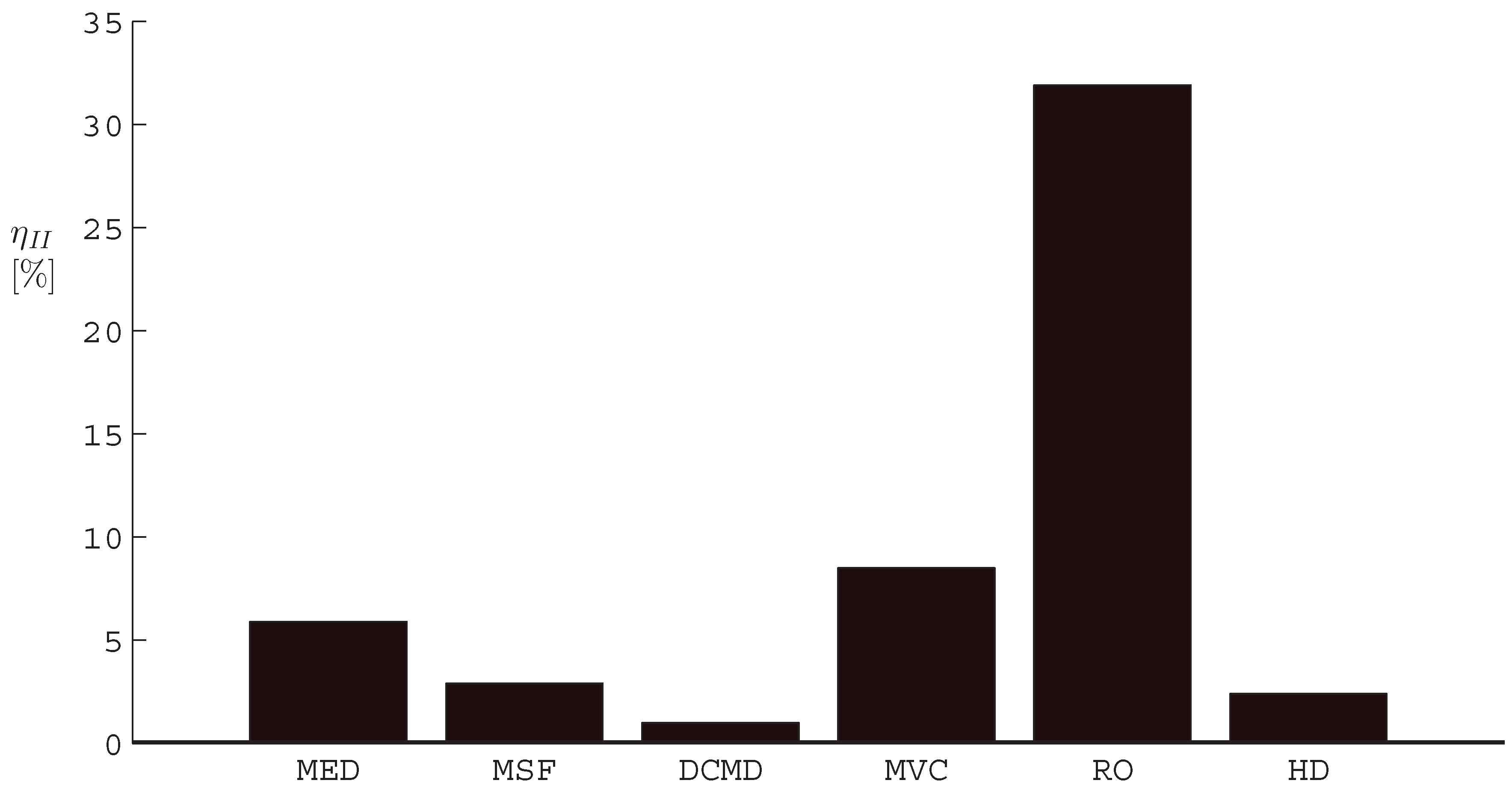
2.2. Second Law Efficiency

The Second Law (or exergetic) efficiency is employed as a measure of the thermodynamic reversibility of a desalination system. Unlike First Law efficiency, which measures the amount of an energy source that is put to use, Second Law efficiency, ${\eta }_{\mathit{II}}$, measures the extent of irreversible losses within a system. A completely reversible system will have a Second Law efficiency of 1 even though the First Law efficiency is likely to be lower. Bejan et al. [14] define the exergetic efficiency as the ratio of the exergy of the process products to the process fuel. In other words, the exergetic efficiency is the ratio of the useful exergy of the outputs of the process (${\dot{\Xi }}_{\text{out,useful}}$) to the exergy of the process inputs (${\dot{\Xi }}_{\text{in}}$):

$${\eta }_{\mathit{II}}\equiv \frac{{\dot{\Xi }}_{\text{out,useful}}}{{\dot{\Xi }}_{\text{in}}}=1-\frac{{\dot{\Xi }}_{\text{destroyed}}+{\dot{\Xi }}_{\text{lost}}}{{\dot{\Xi }}_{\text{in}}}$$

(12)

The second equality in Equation (12) is valid since the useful exergy out is equal to the exergy in minus the sum of the exergy destroyed (${\dot{\Xi }}_{\text{destroyed}}$) and the exergy lost (${\dot{\Xi }}_{\text{lost}}$). Exergy destroyed represents lost available work due to irreversibilities within the system. Exergy lost represents lost available work due to discarding streams to the environment that carry exergy. Note that when the material inputs to the system are taken to be at equilibrium with the environment, ${\Xi }_{\text{in}}$ equals ${\Xi }_{\text{fuel}}$, ${\Xi }_{{\dot{W}}_{\mathrm{sep}}}$, or ${\Xi }_{{\dot{Q}}_{\mathrm{sep}}}$, depending on the energy input. Additionally, Equation (12) is equivalent to the definition used by Kahraman and Cengel [8].

Prior to applying Equation (12) to desalination systems, it is important to understand the differences between the three definitions of work that are presented. The work of separation, ${\dot{W}}_{\mathrm{sep}}$, is the actual amount of work necessary to produce a given amount of water from a fixed feed stream using a real separation process. The least work of separation, ${\dot{W}}_{\mathrm{least}}$, represents the amount of work necessary to produce the same amount of product water from the feed stream while operating under reversible conditions. Finally, the minimum least work, ${\dot{W}}_{\mathrm{least}}^{\min }$, is the minimum required work of separation in the limit of reversible operation and infinitesimal extraction. As a result, the following relation will always hold:

$${\dot{W}}_{\mathrm{sep}}>{\dot{W}}_{\mathrm{least}}(r>0)>{\dot{W}}_{\mathrm{least}}^{\min }(r=0)$$

(13)

In a desalination process, purified water is considered to be the useful product. The useful exergy associated with pure water is the minimum least work (or heat) of separation that is required to obtain purified water from feed water of a given salinity (i.e., infinitesimal extraction of pure water with inlet and outlet streams at ambient temperature). The minimum least work (at zero recovery), rather than the least work (at finite recovery), is used since it represents the actual exergetic value of pure water. To further illustrate, when analyzing a unit of pure water, it is impossible to know the process that was used to produce it. Therefore, the minimum energy required to produce it must be the exergetic value and ${\dot{\Xi }}_{\text{out,useful}}={\dot{W}}_{\mathrm{least}}^{\min }(r=0)$.

Since the control volume is defined so that the inlet stream is at the dead state, the only exergy input to the system comes in the form of either a work (${\dot{W}}_{\mathrm{sep}}$) or heat (${\dot{Q}}_{\mathrm{sep}}$) input (exergy of the feed stream is zero). The work of separation is equivalent to the useful work done within the system plus the exergy destroyed within that system which can be evaluated in one of two ways.

In order to calculate the work of separation, two processes may be considered. The first involves a separation process where the products are brought to thermal and mechanical equilibrium with the environment, whereas the brine is also brought into chemical equilibrium (total dead state, TDS). The reversible work required to achieve this process corresponds to the least work at zero recovery. The total work of separation is given by the sum of the reversible work required plus the exergy destruction associated with entropy generated in the separation and run down to equilibrium processes:

$${\dot{W}}_{\mathrm{sep}}={\dot{W}}_{\mathrm{least}}^{\min }(r=0)+T_0{\dot{S}}_{\mathrm{gen}}^{\text{TDS}}$$

(14)

The second involves a separation process where the products are only brought to thermal and mechanical equilibrium with the environment (restricted dead state, RDS). The reversible work required to achieve this process corresponds to the least work at finite recovery. The total work of separation again is given by the sum of the reversible work required plus the exergy destruction associated with entropy generated in this process:

$${\dot{W}}_{\mathrm{sep}}={\dot{W}}_{\mathrm{least}}(r>0)+T_0{\dot{S}}_{\mathrm{gen}}^{\text{RDS}}$$

(15)

It can be shown that Equations (14) and (15) are equivalent [cf., Section 3.6. Substitution of ${\dot{W}}_{\mathrm{least}}^{\min }$ from Equation (41) into Equation (15) while noting that ${\dot{S}}_{\mathrm{gen}}^{\text{TDS}}={\dot{S}}_{\mathrm{gen}}^{\text{RDS}}+{\dot{S}}_{\mathrm{gen}}^{\mathrm{brine}}\mathrm{RDS}\to \mathrm{TDS}$ exactly gives Equation (14)]. Note that the work of separation for a system can also be directly evaluated using a First Law analysis.

As result, when Equation (12) is applied to a desalination system, it should be written as

$${\eta }_{\mathit{II}}={\displaystyle \frac{{\dot{W}}_{\mathrm{least}}^{\min }}{{\dot{W}}_{\mathrm{sep}}}}={\displaystyle \frac{{\dot{W}}_{\mathrm{least}}^{\min }}{{\dot{W}}_{\mathrm{least}}^{\min }+T_0{\dot{S}}_{\mathrm{gen}}^{\text{TDS}}}}={\displaystyle \frac{{\dot{W}}_{\mathrm{least}}^{\min }}{{\dot{W}}_{\mathrm{least}}+T_0{\dot{S}}_{\mathrm{gen}}^{\text{RDS}}}}$$

(16)

Equation (12) can also be written in terms of the least heat of separation:

$${\eta }_{\mathit{II}}={\displaystyle \frac{{\dot{Q}}_{\mathrm{least}}^{\min }}{{\dot{Q}}_{\mathrm{sep}}}}={\displaystyle \frac{{\dot{Q}}_{\mathrm{least}}^{\min }}{{\dot{Q}}_{\mathrm{least}}^{\min }+{\left(1-\frac{T_0}{T_H}\right)}^{-1}{T}_0{\dot{S}}_{\mathrm{gen}}^{\text{TDS}}}}={\displaystyle \frac{{\dot{Q}}_{\mathrm{least}}^{\min }}{{\dot{Q}}_{\mathrm{least}}+{\left(1-\frac{T_0}{T_H}\right)}^{-1}{T}_0{\dot{S}}_{\mathrm{gen}}^{\text{RDS}}}}$$

(17)

Clearly, the two definitions of Second Law efficiency presented in Equations (16) and (17) are bounded by 0 and 1 because ${\dot{W}}_{\mathrm{sep}}>{\dot{W}}_{\mathrm{least}}$ and ${\dot{Q}}_{\mathrm{sep}}>{\dot{Q}}_{\mathrm{least}}$. Observe that ${\dot{W}}_{\mathrm{least}}$ and ${\dot{Q}}_{\mathrm{least}}$ are functions of feed salinity, product salinity, recovery ratio, and $T_0$. Additionally, ${\eta }_{\mathit{II}}$ will only equal 1 in the limit of completely reversible operation, as expected. Note that the selection of the control volume suitably far away such that all streams are at thermal and mechanical equilibrium allows for this bounding.

It has been shown that there are three relevant Second Law based performance parameters for desalination systems: specific entropy generation, Equation (10); specific exergy destruction, Equation (11); and Second Law efficiency, Equations (16) and (17). This paper will focus on specific entropy generation and Second Law efficiency.

2.3. Energetic Performance Parameters

Three often used parameters are key to describing the energetic performance of desalination systems. The first, called gained output ratio (GOR), is the ratio of the enthalpy required to evaporate the distillate (or equivalently, the energy release in condensation) and the heat input to the system, or

$$\text{GOR}\equiv \frac{{\dot{m}}_p{h}_{(}{T}_0)}{{\dot{Q}}_{\mathrm{sep}}}$$

(18)

In essence, GOR is a measure of how many times the latent heat of vaporization is captured in the condensation of pure water vapor and reused in a subsequent evaporation process to create additional pure water vapor from a saline source. By the First Law of Thermodynamics, a thermal desalination system that has no such heat recovery requires largely the latent heat of vaporization multiplied by the mass of pure water produced as its energy input: its GOR is approximately one. It is important to note that Equation (18) is valid as written only for a desalination system driven by heat; that is, a thermal desalination system. A work-driven desalination system, in contrast, uses electricity or shaft work to drive the separation process. Normally, this work is produced by a thermal process, such as a heat engine. Thus, to evaluate the heat input required for a work-driven desalination system, a First Law efficiency of the process that produces the work of separation must be known.

The second parameter, known as the performance ratio (PR), is defined as the ratio of the mass flow rate of product water to that of the heating steam:

$$\text{PR}\equiv \frac{{\dot{m}}_p}{{\dot{m}}_s}$$

(19)

For a thermal desalination system in which the heat input is provided by condensing steam, as is typical of large-scale thermal processes such as MED and MSF, the values of PR and GOR are quite similar. In that case, the two parameters differ only by the ratio of the latent heat of vaporization at the distillate and heating steam temperatures. That is, GOR = PR $\times \frac{h_{(}{T}_0)}{h_{(}{T}_{\text{steam}})}$.

The third parameter, specific electricity consumption (SEC) is best suited to work-driven desalination systems. It is defined as the ratio of the work of separation (or work input) to the mass flow rate of product water, or

$$\mathrm{SEC}\equiv \frac{{\dot{W}}_{\mathrm{sep}}}{{\dot{m}}_p}$$

(20)

As was the case with GOR, because thermal and electrical energy are not directly comparable, numerical values of SEC cannot be compared between thermal- and work-driven systems without appropriate conversion factors for the work of separation.

3. Analysis of Entropy Generation Mechanisms in Desalination

Several common processes in desalination systems result in entropy generation, including heat transfer, pressure differentials, and non-equilibrium conditions. By utilizing the ideal gas and incompressible fluid models, simple expressions are derived to show the important factors in entropy generation for various physical processes. Details of the derivations may be found in Appendix B and the results are presented below. Physical properties, evaluated at a representative reference state of $50°\mathrm{C}$, are provided in

Table 1. Representative values of reference state constants for Equations (B.3), (B.4), (B.7), and (B.8).

Pure water and vapor constants, $T_{\mathrm{sat}}=50°\mathrm{C}{p}_{\mathrm{sat}}=12.3$ kPa
c	4.18 kJ/kg-K	$h_{\mathrm{ref}}^{\mathrm{IG}}$	2590 kJ/kg
$c_p$	1.95 kJ/kg-K	$h_{\mathrm{ref}}^{\mathrm{IF}}$	209 kJ/kg
R	0.462 kJ/kg-K	$s_{\mathrm{ref}}^{\mathrm{IG}}$	8.07 kJ/kg-K
v	$1.01\times {10}^{-3}$ m3/kg	$s_{\mathrm{ref}}^{\mathrm{IF}}$	0.704 kJ/kg-K
Seawater constants, 50 °C, 35,000 ppm
c	4.01 kJ/kg-K	$h_{\mathrm{ref}}^{\mathrm{IF}}$	200 kJ/kg
v	$0.986\times {10}^{-3}$ m3/kg	$s_{\mathrm{ref}}^{\mathrm{IF}}$	0.672 kJ/kg-K

for pure water [15] and seawater [13]. Proper selection of the reference state is discussed in Appendix B. In all equations in this section, states 1 and 2 are the inlet and outlet states, respectively, for each process.

3.1. Flashing

When liquid water near saturation conditions passes through a throttle, a portion will vaporize as a result of the pressure drop through the device. The exiting fluid, a mixture of vapor and liquid, can be modeled as an ideal gas and incompressible fluid, respectively. The entropy generated in this process is

$$s_{\mathrm{gen}}^{\text{flashing}}=cln\frac{T_2}{T_1}+x\left\{(c_p-c)ln{T}_2-Rln{p}_2+\left[s_{\mathrm{ref}}^{\mathrm{IG}}-s_{\mathrm{ref}}^{\mathrm{IF}}-(c_p-c)ln{T}_{\mathrm{ref}}+Rln{p}_{\mathrm{ref}}\right]\right\}$$

(21)

where the quality, x, is given by:

$$x=\frac{c(T_1-T_2)+v(p_1-p_2)}{(c_p-c)T_2-v{p}_2+[h_{\mathrm{ref}}^{\mathrm{IG}}-h_{\mathrm{ref}}^{\mathrm{IF}}-(c_p-c)T_{\mathrm{ref}}+v{p}_{\mathrm{ref}}]}$$

(22)

and $c_p$ is the specific heat at constant pressure, c is the specific heat of an incompressible fluid, R is the ideal gas constant for steam, v is the specific volume of the liquid, $h_{\mathrm{ref}}^{\mathrm{IG}}$ and $s_{\mathrm{ref}}^{\mathrm{IG}}$ are the enthalpy and entropy for steam at the reference state, and $h_{\mathrm{ref}}^{\mathrm{IF}}$ and $s_{\mathrm{ref}}^{\mathrm{IF}}$ are the enthalpy and entropy for liquid water at the reference state.

3.2. Flow through an Expansion Device without Phase Change

Although the physical causes for pressure drops differ when considering flow through expanders, pipes, throttles, membranes, and other flow constrictions, the control volume equations that govern the entropy generated remains constant.

For an expansion device, the isentropic efficiency, ${\eta }_e$, is defined as:

$${\eta }_e\equiv \frac{w}{w^s}=\frac{h_2-h_1}{h_2^s-h_1}$$

(23)

where w is the work produced per unit mass through the device and $w^s$ is the work produced assuming isentropic expansion.

For entropy generation in the irreversible expansion of an incompressible fluid,

$$s_{\mathrm{gen}}^{\text{expansion,IF}}=cln\left[1+\frac{v}{c{T}_1}(p_1-p_2)\left(1-{\eta }_e\right)\right]\approx \frac{v}{T_1}(p_1-p_2)\left(1-{\eta }_e\right)$$

(24)

In the limit of a completely irreversible pressure drop (such as through a throttle) in which no work is generated, ${\eta }_e=0$ and Equation (24) reduces to:

$$s_{\mathrm{gen}}^{\Delta p,\mathrm{IF}}=cln\left[1+\frac{v}{c{T}_1}(p_1-p_2)\right]\approx \frac{v}{T_1}(p_1-p_2)$$

(25)

For entropy generation in the irreversible expansion of an ideal gas,

$$s_{\mathrm{gen}}^{\text{expansion,IG}}=c_{p}ln\left\{1+{\eta }_e\left[{\left(\frac{p_2}{p_1}\right)}^{R/c_p}-1\right]\right\}-Rln\frac{p_2}{p_1}$$

(26)

In the limit of a completely irreversible pressure drop (such as through a throttle) in which no work is generated, ${\eta }_e=0$ and Equation (26) reduces to:

$$s_{\mathrm{gen}}^{\Delta p,\mathrm{IG}}=-Rln\frac{p_2}{p_1}$$

(27)

Based on Equations (25) and (27), for an incompressible fluid, entropy generation is determined by the pressure difference, whereas for an ideal gas, it is determined by the pressure ratio.

3.3. Pumping and Compressing

For pumping and compressing, the isentropic efficiency, ${\eta }_p$, is defined as:

$${\eta }_p\equiv \frac{w^s}{w}=\frac{h_2^s-h_1}{h_2-h_1}$$

(28)

Entropy generated due to pumping is given by

$$s_{\mathrm{gen}}^{\text{pumping}}=cln\left[1+\frac{v}{c{T}_1}(p_2-p_1)\left(\frac{1}{{\eta }_p}-1\right)\right]\approx \frac{v}{T_1}(p_2-p_1)\left(\frac{1}{{\eta }_p}-1\right)$$

(29)

Entropy generated due to compression is given by

$$s_{\mathrm{gen}}^{\text{compression}}=c_{p}ln\left\{1-\frac{1}{{\eta }_p}\left[1-{\left(\frac{p_2}{p_1}\right)}^{R/c_p}\right]\right\}-Rln\frac{p_2}{p_1}$$

(30)

3.4. Isobaric Heat Transfer Process

In actual heat exchangers, there is always a pressure drop associated with viscous forces. However, without knowledge of specific flow geometry or the local temperature and pressure fields, it is impossible to partition entropy generation according to particular transport phenomena. For example, Bejan [16] has shown that for a simple, single-fluid heat exchanger, comparing the trade off between entropy generation due to heat transfer across a finite temperature difference and pressure drop across a finite flow volume yields an optimum heat exchanger geometry.

In heat exchangers within typical desalination processes, however, the effect of pressure drop on physical properties is insignificant. Thus, entropy generation may be calculated as a function of terminal temperatures alone. For the range of temperatures and flow configurations encountered in the present analysis, this approximation holds for fluids that may be modeled as both ideal gases and incompressible fluids.

The entropy generation equation for a heat exchanger is

$$S_{\mathrm{gen}}^{\mathrm{HX}}={\left[\dot{m}(s_2-s_1)\right]}_{\text{stream}1}+{\left[\dot{m}(s_2-s_1)\right]}_{\text{stream}2}$$

(31)

where, for an ideal gas at an approximately constant pressure, the change in entropy of the stream is

$$s_2-s_1=c_{p}ln\frac{T_2}{T_1}$$

(32)

and for an incompressible fluid, the change in entropy of the stream is

$$s_2-s_1=cln\frac{T_2}{T_1}$$

(33)

For an isobaric phase change from a saturation state (either liquid or vapor), the entropy change is

$$s_2-s_1=x{s}_{\mathit{fg}}=x(s^{\mathrm{IG}}-s^{\mathrm{IF}})\mathrm{for}\text{evaporation}$$

(34)

$$=(x-1)s_{\mathit{fg}}=(x-1)(s^{\mathrm{IG}}-s^{\mathrm{IF}})\mathrm{for}\text{condensation}$$

(35)

where x is the quality at the exit of the process.

3.5. Thermal Disequilibrium of Discharge Streams

Referring again to Figure 1, the entropy generated in bringing outlet streams from the system control volume to the ambient temperature reached at the exit of the distant control volume may be calculated. Consider a stream that is in mechanical, but not thermal equilibrium with the environment (Figure 3). The environment acts as a heat reservoir, and through an irreversible heat transfer process, the stream is brought to thermal equilibrium.

The First and Second Laws for this control volume give:

$$\dot{Q}={\dot{m}}_i(h_i-h_i^{\prime })$$

(36)

$${\dot{S}}_{\mathrm{gen}}={\dot{m}}_i\left[(s_i-s_i^{\prime })-\frac{\dot{Q}}{T_0}\right]={\dot{m}}_i\left[(s_i-s_i^{\prime })-\frac{h_i-h_i^{\prime }}{T_0}\right]$$

(37)

For incompressible fluids at mechanical equilibrium with the environment, $s_i-s_i^{\prime }=c_{i}ln\frac{T_0}{T_i}$ and $h_i-h_i^{\prime }=c_i(T_0-T_i)$. Substituting into Equation (37) gives the entropy generated in bringing a stream of fluid to thermal equilibrium with the environment:

$${\dot{S}}_{\mathrm{gen}}^{T\text{disequilibrium}}={\dot{m}}_i{c}_i\left[ln\left(\frac{T_0}{T_i}\right)+\frac{T_i}{T_0}-1\right]$$

(38)

3.6. Chemical Disequilibrium of Brine Stream

When considering a desalination system, the brine is typically considered to be waste and is discharged back to the ocean. Since the brine is at higher salinity than the ocean, entropy is generated in the process of restoring the brine to chemical equilibrium (also called distributive equilibrium) with the seawater. This entropy generation can be calculated in one of two ways.

First, consider the addition of the concentrated brine stream at the restricted dead state to a large reservoir of seawater at the total dead state. An energy balance governing the mixing of the brine stream with the seawater reservoir is written as follows:

$${\dot{\Xi }}_{\text{destroyed}}^{\text{mixing}}=-[({\dot{m}}_b+{\dot{m}}_{\mathrm{sw}}^{\text{reservoir}})g_{\text{out}}-{\dot{m}}_b{g}_b-{\dot{m}}_{\mathrm{sw}}^{\text{reservoir}}{g}_{\mathrm{sw}}]$$

(39)

where ${\dot{\Xi }}_d^{\text{mixing}}$ is the exergy destroyed as a result of irreversible mixing. In the limit that ${\dot{m}}_B/{\dot{m}}_{\mathrm{sw}}^{\text{reservoir}}\to 0$, $g_{\text{out}}$ approaches $g_{\mathrm{sw}}$ and the brine stream is brought to chemical equilibrium with the environment. Using the Gouy-Stodola theorem [17], the exergy destroyed due to irreversible mixing can be used to evaluate the entropy generated as the brine stream runs down to chemical equilibrium:

$${\dot{S}}_{\mathrm{gen}}^{\mathrm{brine}}\mathrm{RDS}\to \mathrm{TDS}=\frac{{\dot{\Xi }}_{\text{destroyed}}^{\text{mixing}}}{T_0}$$

(40)

The mixing process described by Equation (39) is analogous to the separation process shown in Figure 1 performed in reverse.

A second method to evaluate the entropy generation due to chemical disequilibrium of the brine stream is based on the least work of separation. When considering the control volume given by Figure 1 and the minimum least work of separation, there is an infinitesimally small product stream of pure water along with a stream of brine of salinity that is infinitesimally above that of seawater. Therefore, the brine stream is in thermal, mechanical, and nearly chemical equilibrium with the environment. If, however, there is a finite recovery ratio, the brine stream salinity is greater than that of seawater. Additionally, as the recovery ratio increases, the flow rate of the brine stream decreases and flow rate of the product water increases (assuming fixed input feed rate). Since the brine stream is not at equilibrium with the environment, there is a chemical potential difference that can be used to produce additional work. This additional work is exactly equal to the difference between the least work of separation, Equation (4), and the minimum least work of separation, Equation (6). When the concentrated brine is discarded to the ocean, this work potential is lost. Therefore, entropy generation due to chemical disequilibrium of the brine stream can also be evaluated through the use of the Gouy-Stodola theorem as follows:

$$T_0{\dot{S}}_{\mathrm{gen}}^{\mathrm{brine}}\mathrm{RDS}\to \mathrm{TDS}={\dot{W}}_{\mathrm{least}}(r>0)-{\dot{W}}_{\mathrm{least}}^{\min }(r=0)$$

(41)

Evaluation of entropy generation using Equations (40) and (41) gives equivalent results.

4. Application of Entropy Generation Mechanisms to Seawater Desalination Technologies

Using the methods developed in preceding sections, the component and system level entropy production and the Second Law efficiency of several common seawater desalination technologies are now evaluated.

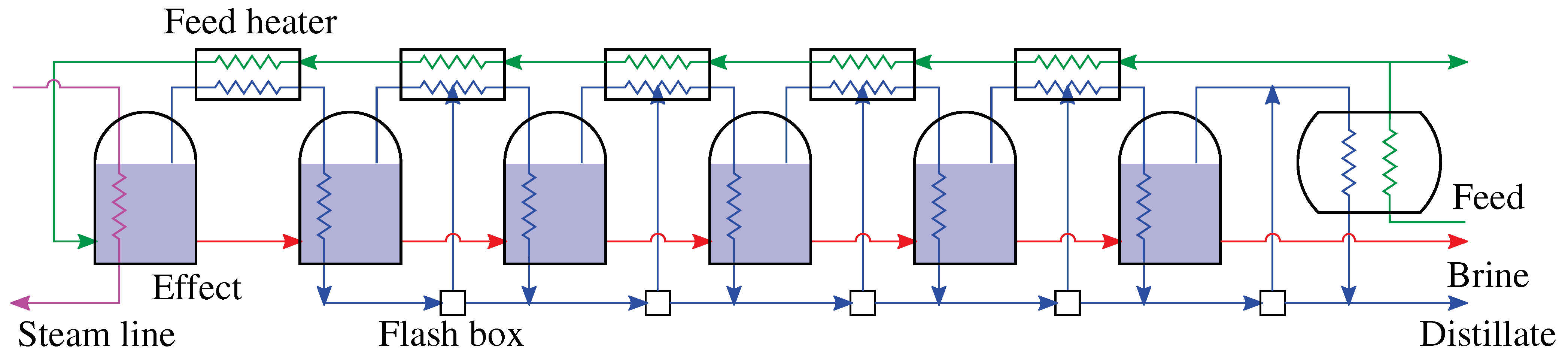
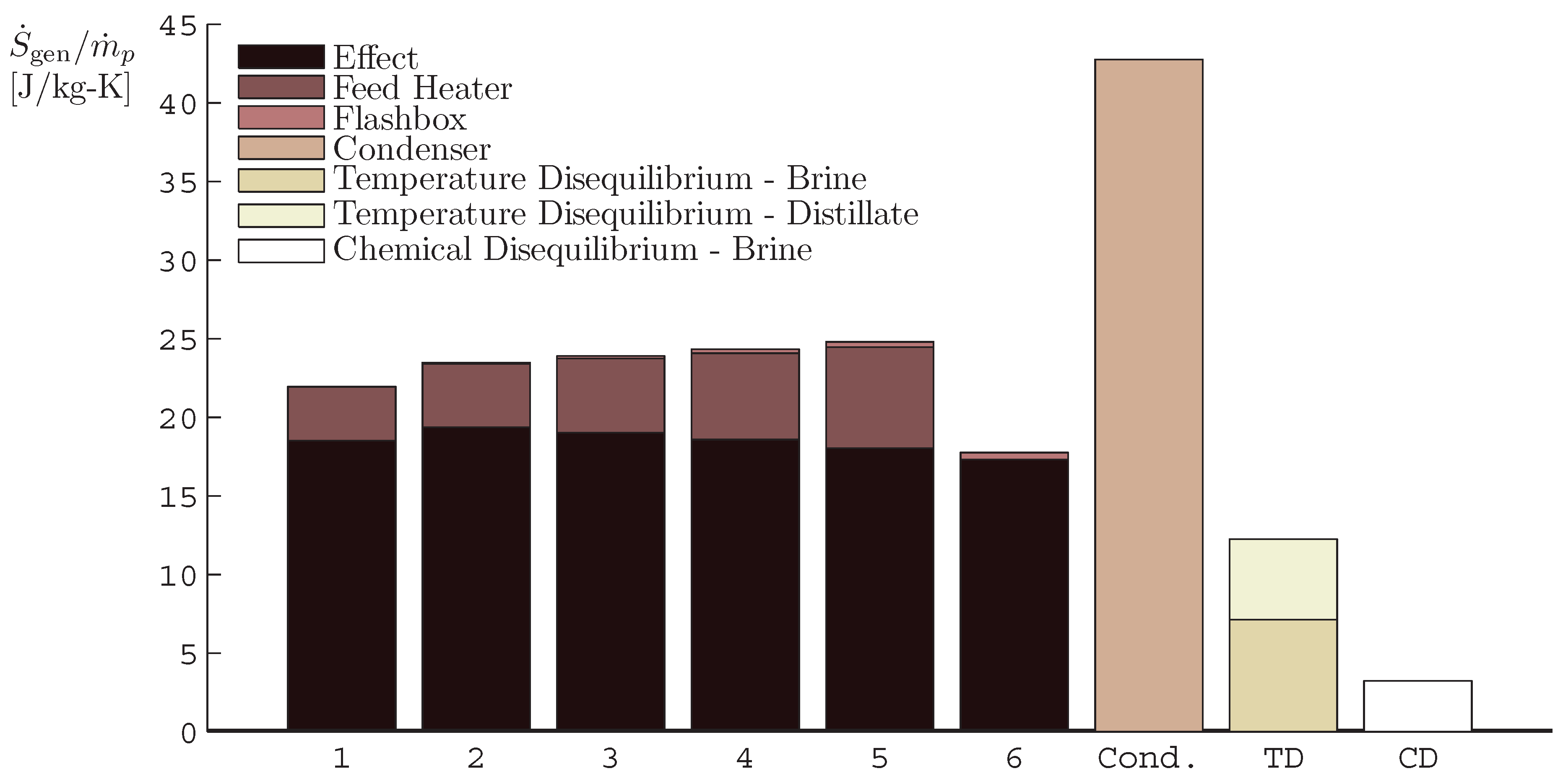
4.1. Multiple Effect Distillation

A very simple model based on approximations from El-Sayed and Silver [18], Darwish et al. [19], and El-Dessouky and Ettouney [20] is used to generate all the temperature profiles and mass flow rates within a multiple effect distillation (MED) forward feed (FF) cycle (Figure 4).

Several common approximations are made: The temperature drop between effects is assumed to be constant, $\Delta T=(T_{\text{steam}}-T_{\text{last}}\text{effect})/n$. Additionally, the driving temperature difference between condensing vapor and evaporating brine and the temperature rise across feed heaters are both taken to be $\Delta T$. The temperature rise in the condenser is set to $10°\mathrm{C}$.

The distillate is approximated as pure water, and it is assumed that distillate is produced in each effect ($D_i$) at a rate of 99% of that produced in the previous effect (i.e., $D_{i+1}=0.99D_i$) to approximate the effect of increasing latent heat with decreasing effect temperature. Distillate produced from flashing in each effect is given by $D_{f,i}={\dot{m}}_{b,i-1}{c}_{p,i}\Delta T/h_{,i}$ where $m_{b,i-1}$ is the brine from the previous effect which becomes the feed to the current effect. The remainder of the distillate is produced from boiling in the effect. There is no flashing in the first effect. Distillate produced from flashing in the flash boxes is given by $D_{fb,i}={\sum }_{j=1}^{i-1}{D}_j{c}_{p,i}\Delta T/h_{,i}$, for $i\ge 2$. The quality of the distillate leaving the feed heater is calculated using an energy balance on the heater, ${\dot{m}}_F{c}_{p,i}\Delta T=(D_i+D_{fb,i})(1-x_i)h_{\mathit{fg}}$, where ${\dot{m}}_F$ is the mass flow rate of the feed seawater.

Water and salinity mass balances for the effects are:

$$\begin{array}{cc}\hfill {\dot{m}}_{b,i-1}& =D_i+{\dot{m}}_{b,i}\hfill \\ \hfill {\dot{m}}_{b,i-1}{y}_{b,i-1}& ={\dot{m}}_{b,i}{y}_{b,i}\hfill \end{array}$$

where $y_{b,i}$ is the salinity of the i^th brine stream.

An energy balance on the first effect gives the required amount of heating steam: ${\dot{m}}_s{h}_{,s}=D_1{h}_{D,1}+{\dot{m}}_{b,1}{h}_{b,1}-{\dot{m}}_F{h}_F$. Accurate properties for seawater [13] and steam [15], including enthalpies, entropies, specific heats, etc., are used and evaluated at each state.

The inputs to the simplified MED FF model with 6 effects include: 1 kg/s of distillate, seawater salinity of 42 g/kg, maximum salinity of 70 g/kg, steam temperature of $70°\mathrm{C}$, last effect temperature of $40°\mathrm{C}$, and seawater (and environment) temperature of $25°\mathrm{C}$.

Using the above approximations and inputs, all thermodynamic states for the MED FF system are found. Entropy generation in each component is computed by using a control volume for each component. Pumping work and entropy generated due to flashing in effects are evaluated using Equations (21) and (29), respectively.

Figure 5 shows the entropy generated in each component, whereas Figure 6 shows the percentage of entropy generated in each type of component. Pumping is not included since the entropy generated due to pumping is much less than 1% of the overall amount. Looking at Figure 6, it is clear that heat transfer is the dominant source of entropy generation in MED systems since most of the generation occurs in the heat exchange devices (effects, feed heaters, and condenser). It was found that entropy generated due to flashing in the effects was very small.

Although the effects result in the greatest portion of the entropy generated, it is important to note that the condenser is the single greatest source of irreversibility, as seen in Figure 5. The condenser is such a large source of entropy generation because very large flow rates of water are needed to condense the vapor from the final effect, and because of the low temperature at which the heat transfer is occurring.

Many modern MED plants operate using a thermal vapor compressor (TVC). The TVC is used to entrain the vapor from the final effect and re-inject it into the first effect. MED-TVC plants have much higher performance ratios than non-TVC plants and they reduce the size of the final condenser, thus reducing this large source of irreversibilities. It is important to note, however, that the TVC is also a highly irreversible device so that total entropy production may not be as much reduced.

Finally, it is seen that for this MED plant, entropy generated as a result of the non-equilibrium discharge of the brine and distillate corresponds to approximately 8.7% of the plant’s overall losses. The Second Law efficiency, accounting for disequilibrium of the discharge, is ${\eta }_{\mathit{II}}=5.9\%$. Additionally, PR = 5.2 and GOR = 5.4.

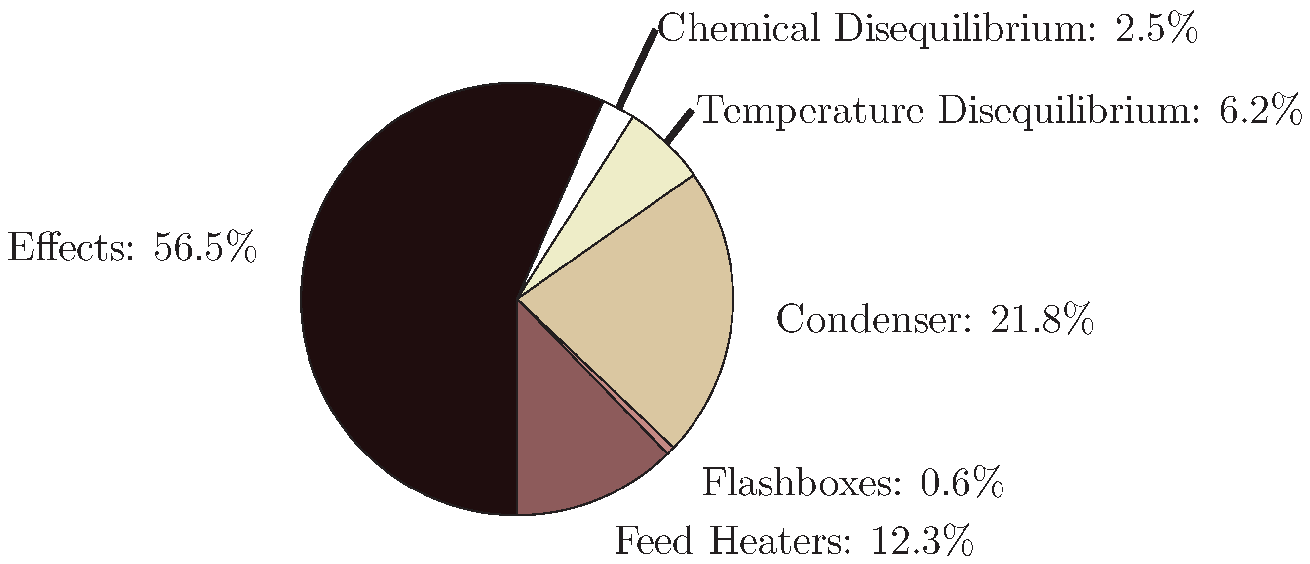
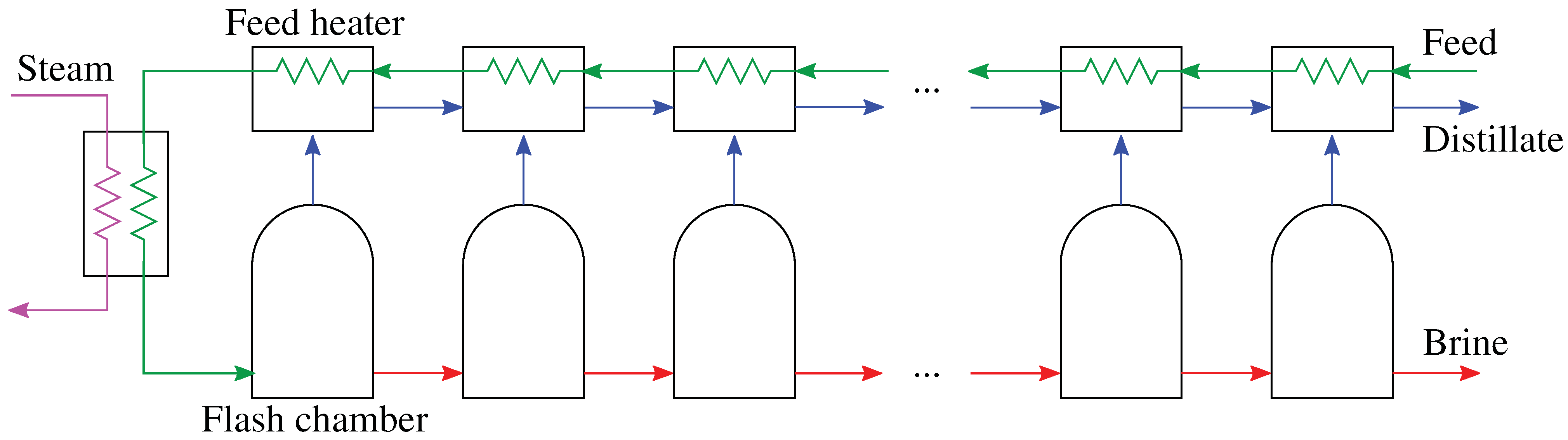
4.2. Multistage Flash

A simple once-through multistage flash (MSF-OT) process with 24 stages is modeled. A schematic diagram of such a process is shown in Figure 7. As is done in several simple MSF modeling schemes [18,20], the stage drop, or difference in sequential flashing chamber saturation temperatures, is assumed to be a constant. Mass and energy balances for each component (brine heater, feed heaters, and flash evaporators) are then solved simultaneously to obtain inlet and outlet conditions for each such component. The mass and energy balances on the i^th feed heater are:

$$\begin{array}{cc}\hfill {\dot{m}}_{d,i}& =D_{f,i}+{\dot{m}}_{d,i-1}\hfill \\ \hfill {\dot{m}}_f(h_{h,i}-h_{h,i-1})& ={\dot{m}}_{d,i}{h}_{d,i}-D_{f,i}{h}_{f,i}-{\dot{m}}_{d,i-1}{h}_{d,i-1}\hfill \end{array}$$

where $D_{f,i}$ is the amount of vapor flashed in the i^th stage. An energy balance on the brine heater is written as ${\dot{m}}_s{h}_{,s}={\dot{m}}_f(h_{b,0}-h_{h,0})$. The required conservation equations for the evaporators are mass, salinity, and energy, respectively given as:

$$\begin{array}{cc}\hfill {\dot{m}}_{b,i-1}& ={\dot{m}}_{b,i}+D_{f,i}\hfill \\ \hfill {\dot{m}}_{b,i-1}{y}_{i-1}& ={\dot{m}}_{b,i}{y}_i\hfill \\ \hfill {\dot{m}}_{b,i-1}{h}_{b,i-1}& ={\dot{m}}_{b,i}{h}_{b,i}+D_{f,i}{h}_{f,i}\hfill \end{array}$$

The inputs to the model are: feed temperature ($25°\mathrm{C}$); steam temperature ($116°\mathrm{C}$); brine reject temperature ($40°\mathrm{C}$); distillate mass flow rate (378.8 kg/s); feed mass flow rate (3384 kg/s); and seawater salinity (42 g/kg). These values are taken from representative MSF-OT data analyzed by El-Dessouky and Ettouney [20].

Table 2. MSF-OT Plant Outputs.

Output		Model Value
Performance ratio	PR	4.2
Gained output ratio	GOR	4.6
Top brine temperature	$T_h$ [°C]	109
Steam flow rate	${\dot{m}}_s$ [kg/s]	91.1
Max salinity	$y_n$ [g/kg]	47.3

displays key outputs from the model; the values agree with the more complex model presented in [20] within 5%. Values of specific enthalpy, specific entropy, and other properties are obtained from [13] for seawater, and [15] for pure water. Results from the present model are given in Table 2.

Applying the definition of Second Law efficiency, Equation (17), to the system yields a value of 2.9%, which is of the same order as the value presented for the similarly large-scale MED system considered in Section 4.1. As can be seen in Figure 8 and Figure 9, the largest source of entropy generation in this particular configuration is the feed heaters, whereas the approximately isothermal evaporators contribute a nearly negligible portion of the plant-wide entropy generation. The relatively small amount of entropy generated in each evaporator is a consequence of the low recovery rate (11%) of the system modeled: the evaporator is approximately isothermal, so the entropy generated is largely the specific entropy of vaporization for a small quantity of flashed vapor. Were the recovery ratio larger and the number of stages similar, more vapor would be flashed in each stage, and entropy generation in the evaporators would increase. Likewise, the dominating portion of entropy generated in the feed heaters can be explained by the low recovery ratio. At low recovery ratios, the circulated brine is the largest thermal mass in the system, and the majority of heat transfer to this stream occurs in the feed heaters.

Including the exergy destruction associated with the temperature disequilibrium between the brine and distillate outputs and the dead state proves to be significant here, accounting for roughly 10% of total entropy production. In particular, the relatively high contribution of the brine disequilibrium to total entropy generation is due to the low recovery ratio inherent in MSF-OT, and the correspondingly high brine reject flow rate that occurs at a temperature significantly above the dead state.

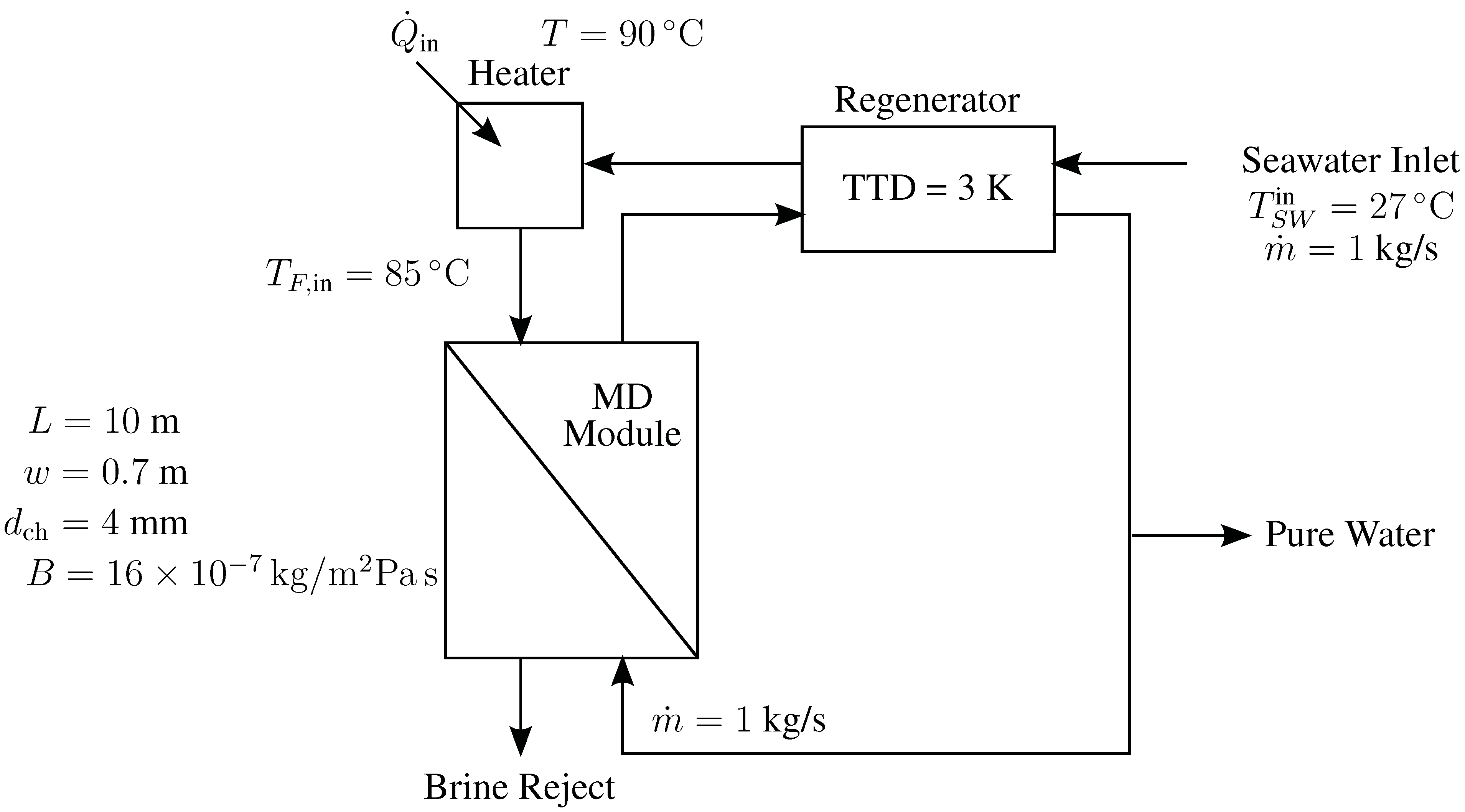
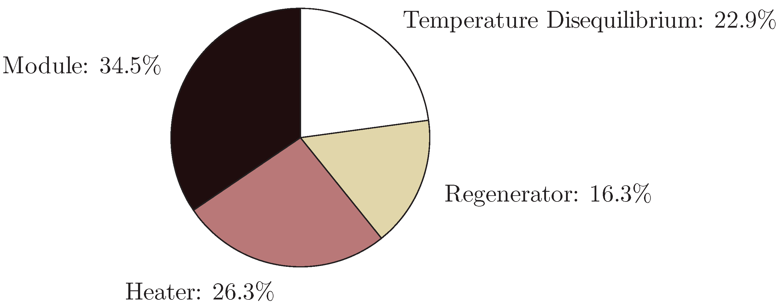
4.3. Direct Contact Membrane Distillation

Direct contact membrane distillation (DCMD) is a membrane-based thermal distillation process in which heated feed passes over a hydrophobic microporous membrane [21]. The membrane holds back a meniscus of water near the pores. On the opposing side, cooled fresh water passes over the membrane. The temperature difference between the water streams induces a vapor pressure difference that drives evaporation through the pores. This can be described in terms of a vapor pressure difference multiplied by a membrane distillation coefficient B, which represents the diffusion resistance through the pores. It is based on material properties, pore geometry, and depends weakly on temperature and is assumed to be constant for this calculation. On the feed side, boundary layers in concentration, temperature, and momentum are present, with corresponding diffusional transport of heat and mass. On the cooler fresh water side, there is condensation of vapor and warming of the fresh water, with boundary layer processes similar to those on the feed side. Direct contact membrane distillation has been successfully used to produce fresh water at small scale (0.1 m³/day) [22,23,24,25].

A transport process model for DCMD based on validated models by Bui et al. [26] and Lee et al. [25] was implemented to obtain the permeate flux, and outlet temperatures of a DCMD module. The calculation of system performance used heat transfer coefficients calculated from correlations based on module geometry [27]. While the Bui et al. [26] model used a hollow-fiber membrane configuration, the present calculations are done for a flat-sheet configuration. Membrane geometry and operating conditions are taken from some pilot-sized plants the literature [28,29]. Seawater enters into the system at $27°\mathrm{C}$ and 35,000 ppm total dissolved solids at a mass flow rate of 1 kg/s, The feed inlet temperature is held constant at $85°\mathrm{C}$, and the required heat is provided by a $90°\mathrm{C}$ source. The permeate side contains fresh water with an inlet flow rate of 1 kg/s. The resulting recovery ratio for this system is 4.4%. The regenerator is a liquid-liquid heat exchanger with a terminal temperature difference of 3 K. The pressure drop through the thin channel in the membrane module was found to be the dominant pressure drop in the system and was the basis for calculating the entropy generation due to pumping power. Properties for seawater [13] were used in the calculation. A schematic diagram of the system is shown in Figure 10, with module geometry and constants shown.

Entropy generation was calculated for each component in the system by using a control volume analysis. Figure 11 shows the breakdown of entropy generation in each component.

The greatest source of entropy generation is the module. This is owed mostly to diffusion through the pores and to a lesser extent heat conduction losses, as only a thin membrane separates the cold and hot streams in the module. The small pore size contributes substantially to the diffusion resistance; the pore diameter is usually on the order of 1000 times less than the membrane thickness. The heater contributes substantially due to the large amount of heat transferred, and the large temperature difference between the source temperature (usually a steam saturation temperature) and the heater inlet. The regenerator has lower entropy generation as it transfers energy through a lower temperature difference, which remains constant throughout its length. The discharge temperature disequilibrium entropy generation is low compared to other thermal systems, as the brine reject temperature is lower. Additionally, since the recovery ratio is low, the chemical disequilibrium of the brine is also found to be negligible (entropy generation due to brine disequilibrium is approximately three orders of magnitude smaller than from other sources). Like most other systems discussed here, the pumping entropy generation was found to be negligible.

Reducing the top temperature, $T_{F,\text{in}}$, results in a net increase in specific entropy generation. This is primarily due to the heater, as a lower top temperature gives rise to a higher temperature difference in the heater. Specific entropy generation in the module goes down slightly, as evaporation happens at a lower temperature; however, this is negated by an increase in specific entropy generation in the regenerator, as water production decreases faster than the temperature gradient in the regenerator. Entropy generation to temperature disequilibrium goes up primarily owing to the lower recovery ratio and additional brine reject.

Given the MD’s low recovery ratio and high discharge temperature, entropy generation is high when compared to other desalination systems, and as a result ${\eta }_{II}=1.0\%$, as calculated with Equation (16) and taking account all sources of entropy generation.

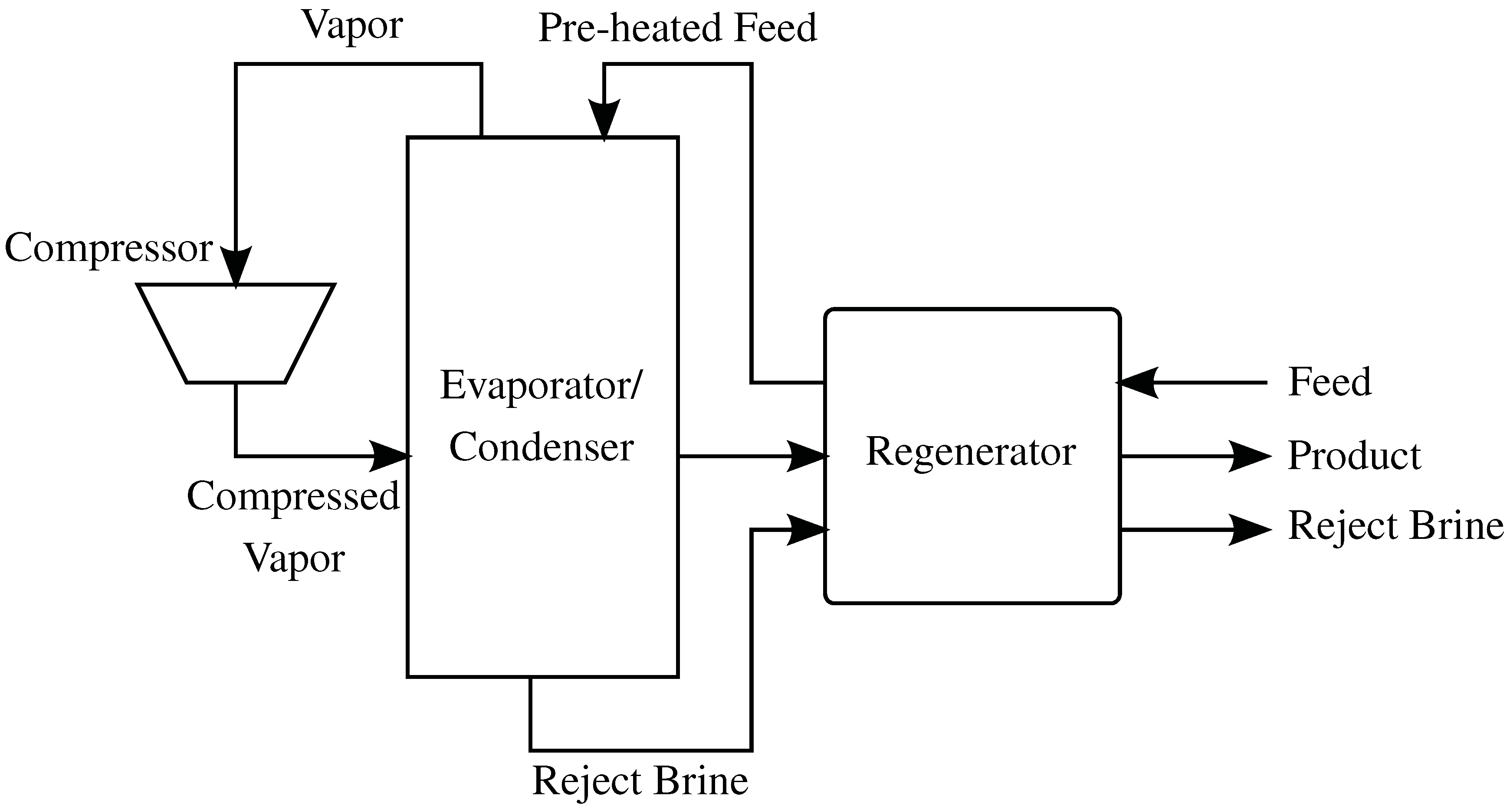
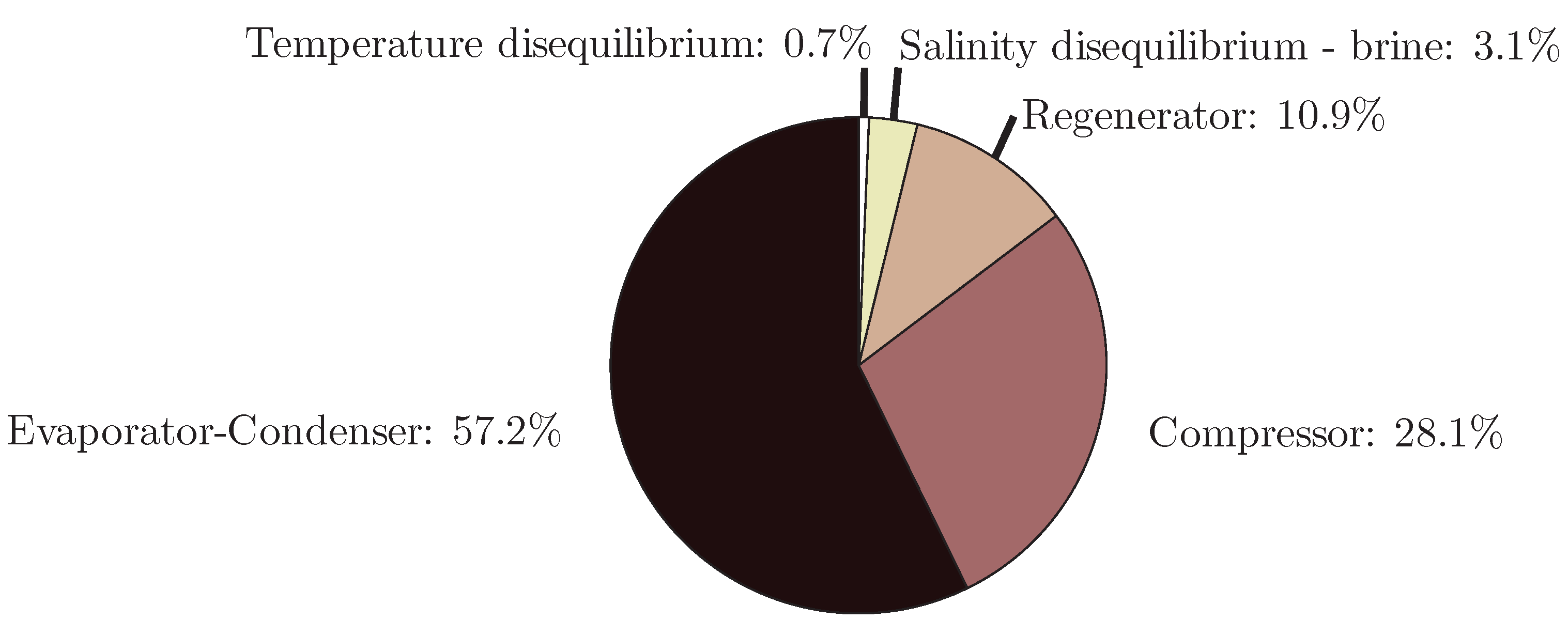
4.4. Mechanical Vapor Compression

A simple single effect mechanical vapor compression (MVC) model is considered. A schematic diagram of the process is shown in Figure 12. The design values chosen for the process are guided by those reported for single stage MVC plants analyzed by Veza [9] and Aly [30] and are listed in

Table 3. MVC design inputs.

Input	Value
Seawater inlet temperature	25 °C
Seawater inlet salinity	35 g/kg
Product water salinity	0 g/kg
Discharged brine salinity	58.33 g/kg
Top brine temperature	60 °C
Pinch: evaporator-condenser	2.5 K
Recovery ratio	40%
Isentropic compressor efficiency	70%
Compressor inlet pressure	19.4 kPa

.

The inlet pressure to the compressor is taken to be the average of the saturation pressure of seawater at a salinity corresponding to the average of the feed and reject salinity. The regenerating heat exchanger is thermally balanced and thus the temperature difference is taken to be constant between the rejected brine and the feed stream and also between the product water and the feed stream. By employing energy conservation equations for each component, the unknown thermodynamic states may be computed. Knowing the thermodynamic states at each point, the entropy generated within each component may be calculated along with the entropy generated when the discharged brine is returned to a body of water with the same composition and temperature as the feed. The key outputs from the model are reported in

Table 4. MVC model outputs.

Output	Value
Specific electricity consumption	8.84 kWh/m3
Discharged brine temperature	27.2 °C
Product water temperature	29.7 °C
Compression ratio	1.15
Second Law efficiency, ${\eta }_{\mathit{II}}$	8.5%

. The breakdown of entropy generation among components is indicated within Figure 13.

The majority of entropy generation may be attributed to heat transfer across a finite temperature difference from the condensation process to the evaporation process. Entropy generation within the regenerator is less significant, primarily because the sensible heat transferred in the regenerator is substantially smaller than the large amount of latent heat recovered in the evaporator-condenser. Entropy generation due to irreversibility within the compressor is important and depends upon the compression ratio and its isentropic efficiency. Entropy generated in returning concentrated brine to a body of seawater is considerable as the recovery ratio is high (40%). Entropy generated in returning product streams to the temperature of inlet seawater is small as the regenerator is effective in bringing these streams to a temperature close to that of the inlet seawater.

The MVC system modeled above is a simple single effect system, satisfactory for demonstrating the distribution of entropy generation throughout MVC plants. Detailed thermoeconomic models with multiple effects have been analyzed in literature [31]. Research has also been undertaken on improving the heat transfer coefficients within the evaporation and condensation processes of phase change. Lara et al. [32] investigated high temperature and pressure MVC, where dropwise condensation can allow greatly enhanced heat transfer coefficients. Lukic et al. [33] also investigated the impact of dropwise condensation upon the cost of water produced. Such improvements in heat transfer coefficients reduce the driving temperature difference in the evaporator-condenser leading to a lower compression ratio and thus reduced compressor work requirements per unit of water produced. As the present analysis shows, reduction of entropy generation within the evaporator-condenser and the compressor are crucial if exergetic efficiency is to be improved upon.

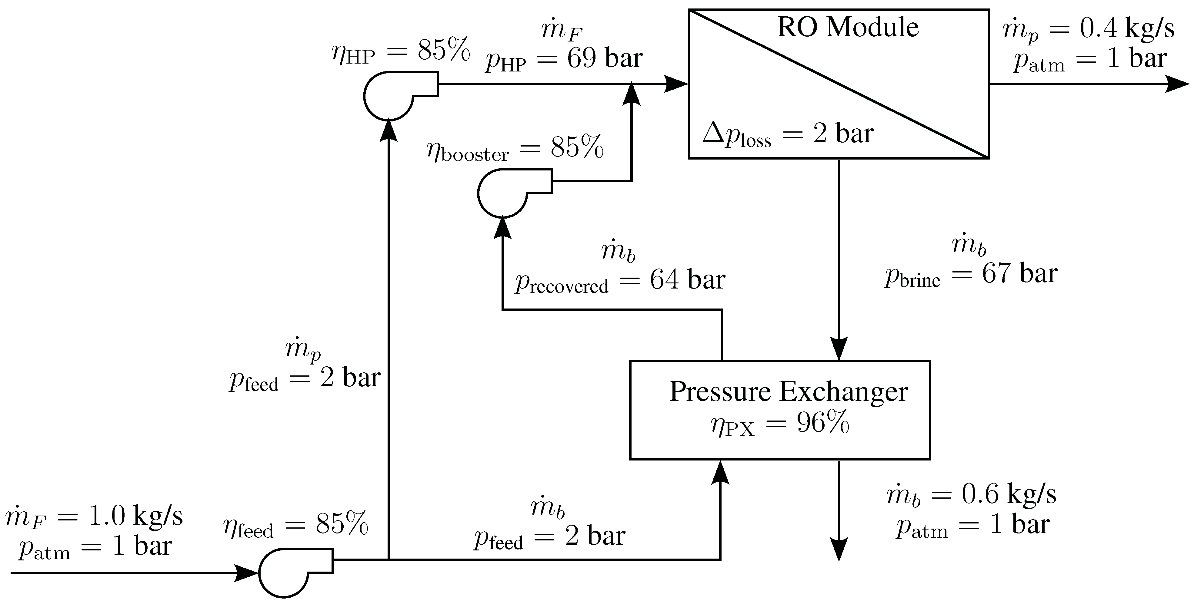
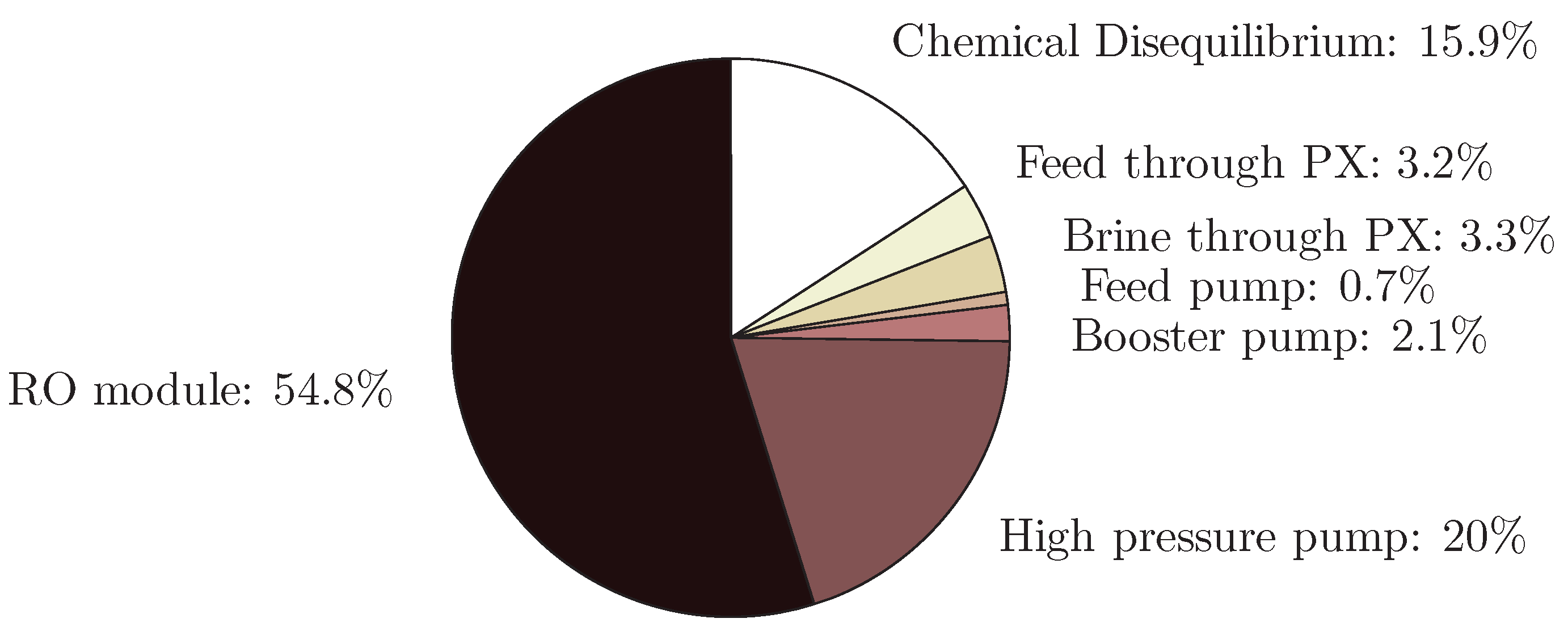
4.5. Reverse Osmosis

A typical flow path for a single stage reverse osmosis (RO) plant with energy recovery is shown in Figure 14 [34]. Since RO is a mechanically driven system and thermal effects are of second order to pressure effects, reasonably accurate calculations can be performed while only considering pressure work. The following approximations are made:

Feed seawater is assumed to enter at ambient temperature and pressure ($25°\mathrm{C}$, 1 bar) and at standard seawater salinity (35 g/kg). Pure water (0 g/kg salinity) is assumed to be produced at a recovery ratio of 40%. Further, it is assumed that 40% of the feed is pumped to 69 bar using a high pressure pump while the remaining 60% is pumped to the same pressure using a combination of a pressure exchanger driven by the rejected brine as well as a booster pump. The high pressure, booster, and feed pump efficiencies are assumed to be 85%. The concentrated brine loses 2 bar of pressure through the RO module while the product leaves the module at 1 bar. Energy Recovery Inc. [35] makes a direct contact pressure exchanger that features a single rotating part. The pressure exchanger pressurizes part of the feed using work produced through the depressurization of the brine in the rotor. Equations (23), (28), and (B.3) are used to match the work produced in expansion to the work required for compression. Assuming the expansion and compression processes are 98% efficient [35], the recovered pressure is calculated as follows:

$$p_{\text{recovered}}=p_{\text{feed}}-{\eta }_{\text{expansion}}{\eta }_{\text{compression}}\left(\frac{{\rho }_{\text{feed}}}{{\rho }_{\text{brine}}}\right)\left(p_{\text{brine}}-p_{\text{atm}}\right)$$

(42)

and the pressure exchanger efficiency is evaluated using ERI’s definition [34]:

$${\eta }_{\text{PX}}={\displaystyle \frac{{\sum }_{\text{out}}\mathrm{Pressure}\times \mathrm{Flow}}{{\sum }_{\text{in}}\mathrm{Pressure}\times \mathrm{Flow}}}$$

(43)

Density of seawater is evaluated using seawater properties [13].

Using the above assumptions, approximations, and inputs, the entropy generated in the various components can be directly calculated using equations derived in Section 3. The entropy generated in the high pressure pump, booster pump, and the feed in the pressure exchanger is evaluated using Equation (29). The entropy generated through the expansion of the pressurized brine in the pressure exchanger is evaluated using Equation (24).

Additional consideration is necessary for the entropy generation in the RO module because both the mechanical and chemical state of the seawater is changing. Since entropy is a state variable, the process can be decomposed into two sub-processes for the purpose of calculating the overall change of state. First, the high pressure seawater is isobarically and isothermally separated into two streams of different composition. Next, the two streams are depressurized at constant salinity in order to account for the pressure drop associated with diffusion through the membrane (product, $\Delta p=68$ bar) and that associated with hydraulic friction (brine, $\Delta p=2$ bar).

In order to evaluate the entropy change as a result of the separation process, the physical properties of seawater are needed as function of temperature, pressure, and salinity. For the model of separation considered here, the compositional change is taken at constant high pressure and temperature, so that the entropy change due to compositional change is easily evaluated:

$$\Delta {\dot{S}}_{\text{composition}}={\dot{m}}_p{s}_p(T_0,p_{\mathrm{HP}},y_p)+{\dot{m}}_b{s}_p(T_0,p_{\mathrm{HP}},y_p)-{\dot{m}}_F{s}_F(T_0,p_{\mathrm{HP}},y_F)$$

(44)

Since seawater is nearly incompressible, entropy is independent of p, and can be evaluated using the property package developed by Sharqawy et al. [13] (which does not currently include pressure effects). Note that $\Delta {\dot{S}}_{\text{composition}}\approx -{\dot{W}}_{\mathrm{least}}(r>0)/T_0$ since ${\dot{W}}_{\mathrm{least}}(r>0)=\Delta {\dot{G}}_{\text{composition}}=\Delta {\dot{H}}_{\text{composition}}-T\Delta {\dot{S}}_{\text{composition}}$ [cf., Equation (4)] and $\Delta {\dot{H}}_{\text{composition}}$ is small.

Entropy generation due to the irreversible depressurization of both the brine and product streams is evaluated through the use of Equation (25). The total entropy generated in the RO module is the sum of the entropy change due to compositional changes, Equation (44), and the entropy generated in the depressurization of the product and brine streams, Equation (25).

The energy dissipated by pressure loss and pump inefficiency results in very small increases in the system temperature. As a result, the entropy generation associated with the transfer of this energy out of the system as heat (if any) through the very small temperature difference from the environment is negligible relative to the mechanical sources of entropy production [see Equation (38)].

Figure 15 is a pie chart showing the relative amounts of entropy generation within the single stage RO system. The greatest irreversibility occurs within the RO module. Further examining the entropy generation in the RO module, it is found that ${\dot{S}}_{\mathrm{gen}}$ from the depressurization of the product is 22.6 J/kg_product-K, while ${\dot{S}}_{\mathrm{gen}}$ from the depressurization of the brine is only 1.0 kJ/kg_product-K; the entropy change from compositional change is $-12.9$ J/kg_product-K. Therefore, the diffusion of water through the RO membrane is the largest source of irreversibility, owing mainly to the large pressure drop (68 bar). Note that the high pressure pump handles the same flow rate of water through the same pressure difference, but does so at 85% efficiency and therefore generates substantially less entropy than the (zero efficiency) flow through the membrane.

Based on these conditions, the minimum least work is found to be 2.71 kJ/kg and the total entropy generation is 19.4 J/kg-K. Therefore, the required work of separation is 8.50 kJ/kg (2.35 kWh/m³) and the Second Law efficiency, per Equation (16), is 31.9%.

Since RO systems tend to operate at higher Second Law efficiency than thermal plants, the irreversibility due to discharge disequilibrium of the brine stream has a larger contribution to the total entropy generation. As seen in Figure 15, the high salinity of the brine accounts for almost 16% of the plant’s total irreversibility. The only way to reduce this effect is to lower the recovery ratio or to implement an osmotic power recovery device on the reject brine stream.

When trying to improve RO systems, designers target the irreversibilities in the module. The simplest way to improve the performance of the system is to use a two (or more) stage RO system (e.g., as described by Elimelech and Phillip [36]). In a two stage system, water is extracted at a lower recovery ratio from the first stage, resulting in a lower brine concentration. Since the required pressure of the feed is dependent on the osmotic pressure, which itself is a function of the feed concentration, a lower recovery ratio means that lower pressures are needed in the first stage. Next, the brine from the first stage is then further pressurized to the top pressure and additional water is extracted in a second stage. Even though the same top pressure is reached, since the flow rates at the highest pressure are smaller, less total entropy is generated in the two stage system. Batch processing of seawater, as done by Desalitech Ltd. [37], also serves to reduce the volume of water that needs to be pressurized to the maximum pressure.

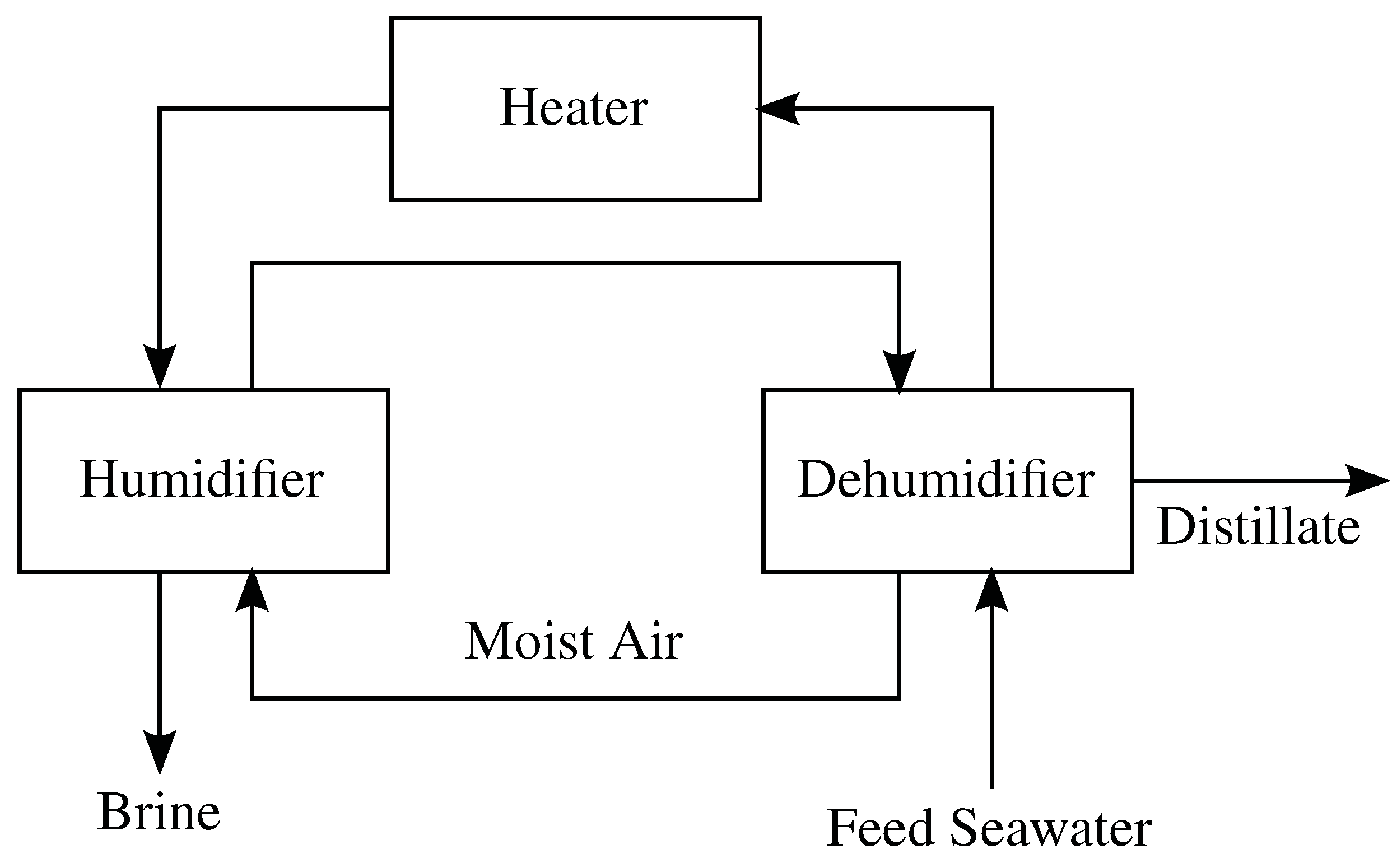
4.6. Humidification-Dehumidification

A solar driven closed air open water (CAOW) humidification-dehumidification (HD or HDH) desalination cycle with water heating (WH) is modeled [6,38,39,40,41,42]. A schematic diagram of the CAOW-WH HD cycle is shown in Figure 16. Specifically, the model developed by Mistry et al. [38] is used with additional equations added to calculate entropy generation due to temperature and chemical disequilibrium as well as Second Law efficiency.

In this model, all components are modeled as black boxes. The humidifier and dehumidifier are characterized by an effectiveness parameter designed to capture the effects of simultaneous heat and mass transfer [43]. The solar heater is approximated as a constant heat flux surface. Pumping losses are ignored since all streams are approximated to be at atmospheric pressure. Physical properties are evaluated for seawater [13], moist air [44], and pure water [45].

Operating conditions are selected as: mass flow rate ratio of seawater to dry air is 3; effectiveness of the humidifier and dehumidifier is 90%; seawater temperature and salinity are $30°\mathrm{C}$ and 35 g/kg respectively; and brine top temperature is $70°\mathrm{C}$. A breakdown of the contributions to the entropy generation for the CAOW-WH HD cycle is shown in Figure 17. For this example, the dehumidifier is the limiting component as it is the greatest source of irreversibility. Further discussion regarding the sources of irreversibility within the components is provided in [38].

Entropy generation due to thermal disequilibrium accounts for approximately 16% of the total irreversibility in the system. As with the MSF-OT and DCMD systems considered earlier, the low recovery ratio (4.5%) results in very low entropy generation due to chemical disequilibrium of the brine. Based on these conditions, the minimum least work is 2.76 kJ/kg and the total entropy generation is 370 J/kg-K. Therefore, the required heat of separation is 962 kJ/kg (GOR is 2.5) and the Second Law efficiency is 2.4%.

Mistry et al. [6] performed an exergy analysis of a wide range of CAOW HD cycle configurations (water heated, air heated) at various operating conditions (top temperature, mass flow rate ratio, component effectiveness, etc.) and found that there was no consistent correlation between a cycle’s exergetic efficiency and GOR (see [6], Table 1 and Figure 10). In addition to the reasons discussed in [6], the lack of consistent correlation between the two parameters is largely a result of defining ${\eta }_{\mathit{II}}$ as ${\dot{\Xi }}_{\text{out}}/{\dot{\Xi }}_{\text{in}}$ rather than ${\dot{\Xi }}_{\text{out,useful}}/{\dot{\Xi }}_{\text{in}}$. Accounting for the exergy lost in the discarded streams (i.e., exergy destroyed due to thermal and chemical disequilibrium) in the definition of ${\eta }_{\mathit{II}}$, as discussed in Section 2.2, reconciles the inconsistencies that were observed. The original data from ([6], Figure 10) is provided in Figure 18a. Additionally, the data is plotted against the proper definition of Second Law efficiency, Equation (17), in Figure 18b and it is seen that there is a definite positive correlation between GOR and ${\eta }_{\mathit{II}}$, regardless of the cycle configuration or operating conditions, as expected.

5. Conclusions

In this paper, the following conclusions have been reached:

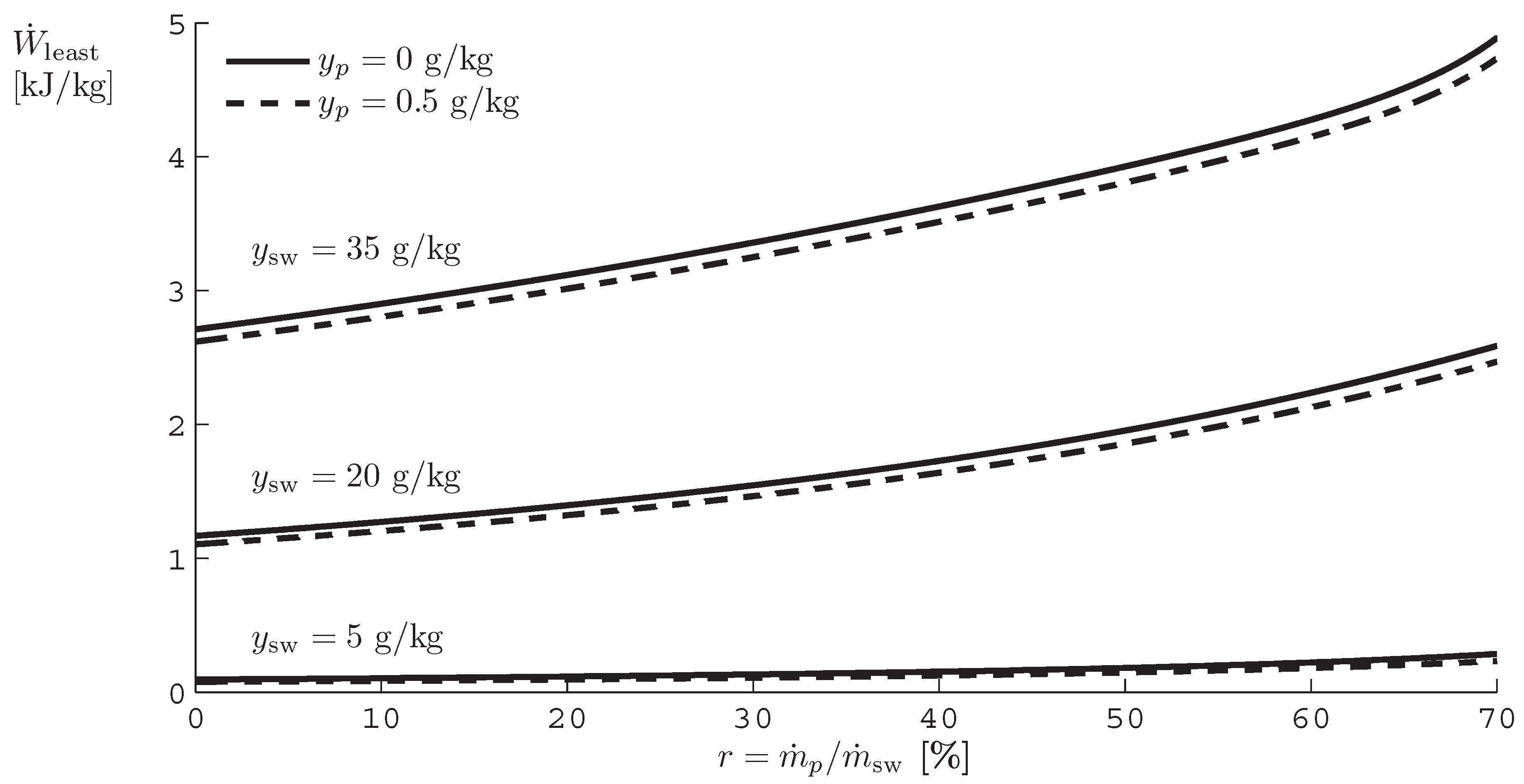
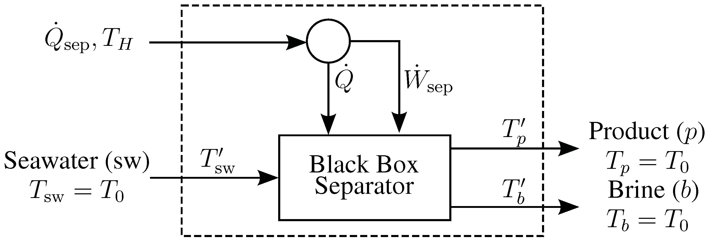
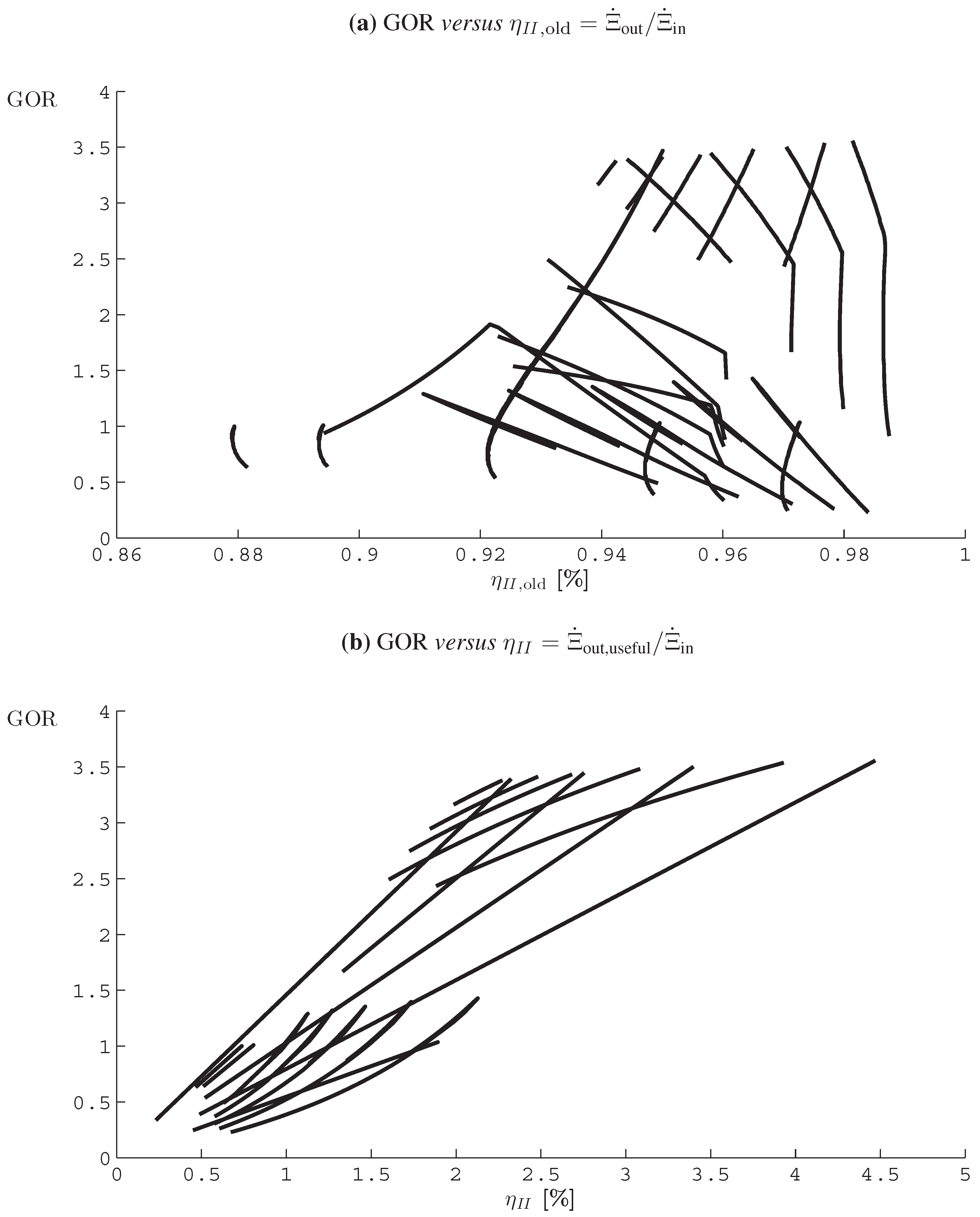
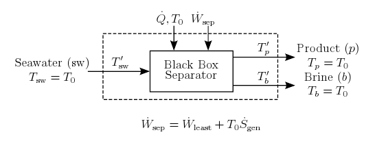
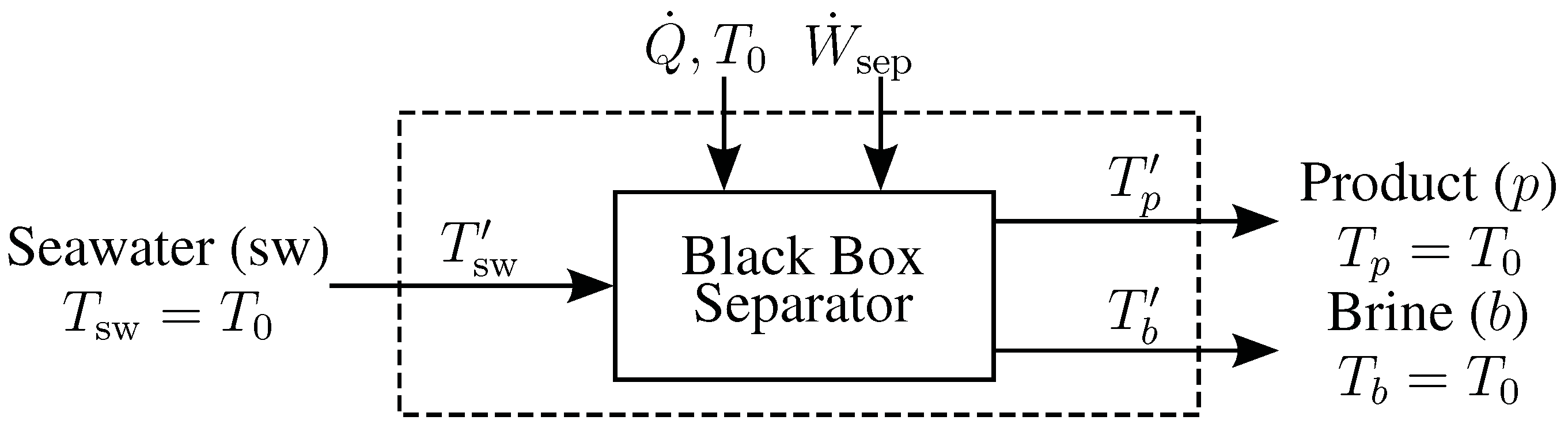
• A Second Law efficiency is developed for desalination systems and is defined as the useful work output divided by the total work input to the system. The useful work output of a desalination system is the minimum least work of separation, since the useful output of the system is pure water, not pure hot water. Minimum least work of separation is defined such that all input and output streams with exception of the product stream are in thermal, mechanical, and chemical equilibrium with the environment (total dead state). The product stream is in thermal and mechanical equilibrium with the environment (restricted dead state). The exergy input to the desalination systems analyzed is either in the form of work or heat. See Equation (16).
• When considering the work input to be the minimum least work of separation plus lost work due to entropy generation, it is essential to consider entropy generated not only due to irreversibilities in the separation process, but also due to temperature disequilibrium of the discharge and the irreversible mixing of the brine with the ambient seawater. See Equation (14).
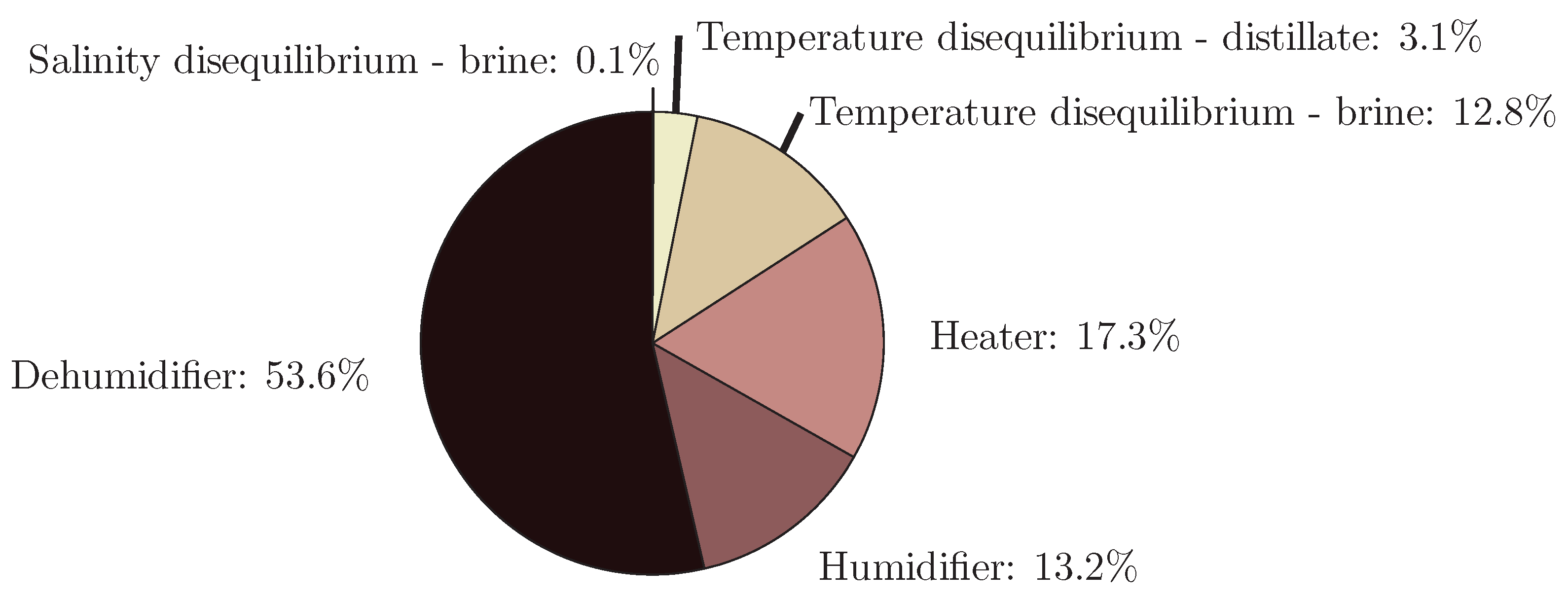
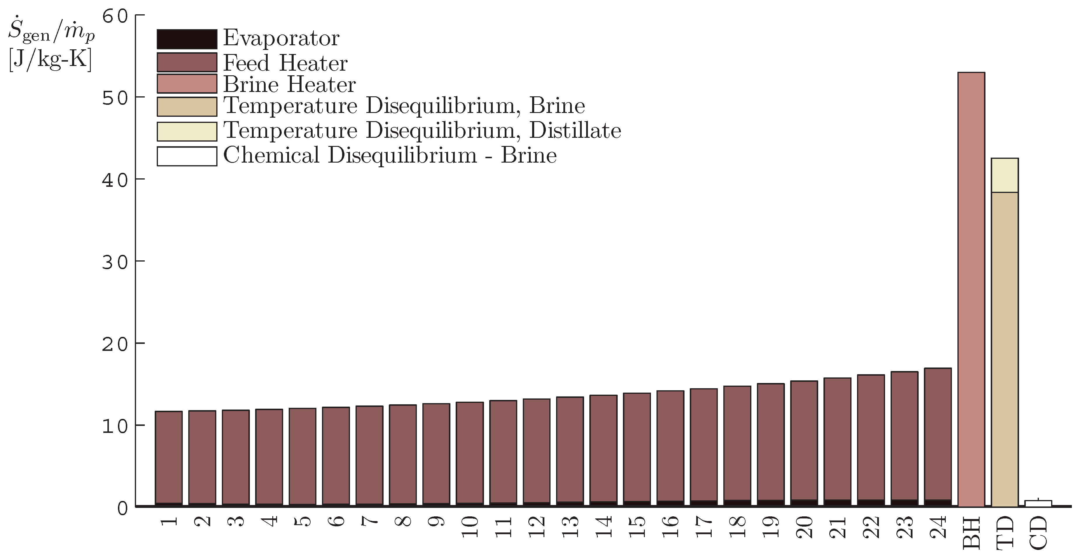
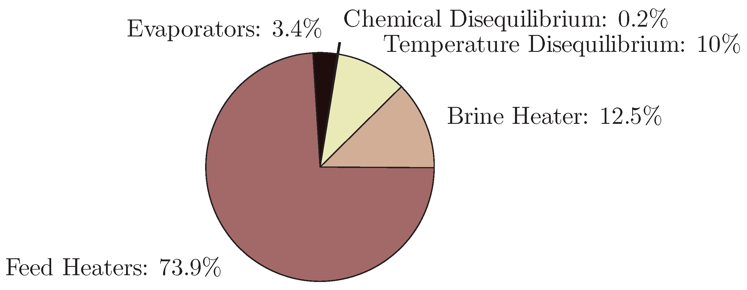
• The application of entropy generation analysis to various desalination technologies showed that thermal disequilibrium of the discharge streams results in a substantial portion of the entropy generated in thermal systems. Similarly, it was seen that entropy generation due to chemical disequilibrium is important only in systems with high recovery ratios. Depending on whether thermal or chemical disequilibrium is important, modifications to the systems can be implemented in order to capitalize on the potential differences between the discharge streams and the environment and reduce the required energy input.

The entropy generation techniques discussed herein provide a useful set of tools for analyzing desalination systems in order to determine major sources of lost work. However, it is important to note that entropy generation analysis is primarily useful for understanding how to improve a specific system. Comparing Second Law efficiency of various systems (e.g., MED vs. RO) only shows which system is operating closer to the reversible limit (Figure 19). While this is useful for understanding which systems have the potential for further improvement, it is often more useful, for system engineering purposes, to compare ${\eta }_{\mathit{II}}$ of a single system operating under various conditions since this allows a designer to understand the irreversibilities within a system. One should be careful when comparing ${\eta }_{\mathit{II}}$ for systems with electrical energy input to those with thermal energy input. Electricity is a higher grade energy source than heat, and additional entropy is generated in the conversion from heat (or fuel) to electricity.

References

1. Oki, T.; Kanae, S. Global hydrological cycles and world water resources. Science 2006, 313, 1068–1072. [Google Scholar] [CrossRef] [PubMed]
2. Smakhtin, V.; Revenga, C.; Döll, P. Taking into account environmental water requirements in global-scale water resources assessments. In Comprehensive Assessment Research Report 2; Comprehensive Assessment Secretariat, International Water Management Institute: Colombo, Sri Lanka, 2004. [Google Scholar]
3. Shannon, M.A.; Bohn, P.W.; Elimelech, M.; Georgiadis, J.G.; Marinas, B.J.; Mayes, A.M. Science and technology for water purification in the coming decades. Nature 2008, 452, 301–310. [Google Scholar] [CrossRef] [PubMed]
4. Semiat, R. Energy issues in desalination processes. Environ. Sci. Tech. 2008, 42, 8193–8201. [Google Scholar] [CrossRef]
5. Spiegler, K.S.; El-Sayed, Y.M. The energetics of desalination processes. Desalination 2001, 134, 109–128. [Google Scholar] [CrossRef]
6. Mistry, K.H.; Lienhard V, J.H.; Zubair, S.M. Effect of entropy generation on the performance of humidification-dehumidification desalination cycles. Int. J. Therm. Sci. 2010, 49, 1837–1847. [Google Scholar] [CrossRef]
7. Alasfour, F.; Darwish, M.; Amer, A.B. Thermal analysis of ME–TVC+MEE desalination systems. Desalination 2005, 174, 39–61. [Google Scholar] [CrossRef]
8. Kahraman, N.; Cengel, Y.A. Exergy analysis of a MSF distillation plant. Energ. Convers. Manag. 2005, 46, 2625–2636. [Google Scholar] [CrossRef]
9. Veza, J.M. Mechanical vapour compression desalination plants—A case study. Desalination 1995, 101, 1–10. [Google Scholar] [CrossRef]
10. Cerci, Y. Exergy analysis of a reverse osmosis desalination plant in California. Desalination 2002, 142, 257–266. [Google Scholar] [CrossRef]
11. Sharqawy, M.H.; Zubair, S.M.; Lienhard V, J.H. Second Law analysis of reverse osmosis desalination plants: An alternative design using pressure retarded osmosis. Energy 2011, in press. [Google Scholar] [CrossRef]
12. Sharqawy, M.H.; Lienhard V, J.H.; Zubair, S.M. On exergy calculations of seawater with applications in desalination systems. Int. J. Therm. Sci. 2011, 50, 187–196. [Google Scholar] [CrossRef]
13. Sharqawy, M.H.; Lienhard V, J.H.; Zubair, S.M. Thermophysical properties of seawater: A review of existing correlations and data. Desalination and Water Treatment 2010, 16, 354–380. [Google Scholar] [CrossRef]
14. Bejan, A.; Tsatsaronis, G.; Moran, M. Themal Design and Optimization; John Wiley & Sons, Inc.: New York, NY, USA, 1996. [Google Scholar]
15. Wagner, W.; Pruss, A. The IAPWS formulation 1995 for the thermodynamic properties of ordinary water substance for general and scientific use. J. Phys. Chem. Ref. Data 2002, 31, 387–535. [Google Scholar] [CrossRef]
16. Bejan, A. General criterion for rating heat-exchanger performance. Int. J. Heat. Mass Tran. 1978, 21, 655–658. [Google Scholar] [CrossRef]
17. Bejan, A. Advanced Engineering Thermodynamics, 3rd ed.; John Wiley & Sons, Inc.: Hoboken, NJ, USA, 2006. [Google Scholar]
18. El-Sayed, Y.M.; Silver, R.S. Principles of Desalination; Academic Press: New York, NY, USA, 1980; Volume A, Chapter Fundamentals of Distillation; pp. 55–109. [Google Scholar]
19. Darwish, M.; Al-Juwayhel, F.; Abdulraheim, H.K. Multi-effect boiling systems from an energy viewpoint. Desalination 2006, 194, 22–39. [Google Scholar] [CrossRef]
20. El-Dessouky, H.T.; Ettouney, H.M. Fundamentals of Salt Water Desalination; Elsevier: Amsterdamn, The Netherlands, 2002. [Google Scholar]
21. Lawson, K.W.; Lloyd, D.R. Membrane distillation. J. Membr. Sci. 1997, 124, 1–25. [Google Scholar] [CrossRef]
22. Rodriguez-Maroto, J.; Martinez, L. Bulk and measured temperatures in direct contact membrane distillation. J. Membr. Sci. 2005, 250, 141–149. [Google Scholar] [CrossRef]
23. Martinez-Diez, L.; Florido-Diaz, F.J. Desalination of brines by membrane distillation. Desalination 2001, 137, 267–273. [Google Scholar] [CrossRef]
24. Song, L.; Li, B.; Sirkar, K.K.; Gilron, J.L. Direct contact membrane distillation-based desalination: Novel membranes, devices, larger-scale studies, and a model. Ind. Eng. Chem. Res. 2007, 46, 2307–2323. [Google Scholar] [CrossRef]
25. Lee, H.; He, F.; Song, L.; Gilron, J.; Sirkar, K.K. Desalination with a cascade of cross-flow hollow fiber membrane distillation devices integrated with a heat exchanger. AIChE J. 2011, 57, 1780–1795. [Google Scholar] [CrossRef]
26. Bui, V.; Vu, L.; Nguyen, M. Modelling the simultaneous heat and mass transfer of direct contact membrane distillation in hollow fibre modules. J. Membr. Sci. 2010, 353, 85–93. [Google Scholar] [CrossRef]
27. Lienhard IV, J.H.; Lienhard V, J.H. A Heat Transfer Textbook, 4th ed.; Dover Publications: Mineola, NY, USA, 2011. [Google Scholar]
28. Fath, H.E.; Elsherbiny, S.M.; Hassan, A.A.; Rommel, M.; Wieghaus, M.; Koschikowski, J.; Vatansever, M. PV and thermally driven small-scale, stand-alone solar desalination systems with very low maintenance needs. Desalination 2008, 225, 58–69. [Google Scholar] [CrossRef]
29. Banat, F.; Jwaied, N.; Rommel, M.; Koschikowski, J.; Wieghaus, M. Desalination by a “compact SMADES” autonomous solar-powered membrane distillation unit. Desalination 2007, 217, 29–37. [Google Scholar] [CrossRef]
30. Aly, S.E. Gas turbine total energy vapour compression desalination system. Energ. Convers. Manag. 1999, 40, 729–741. [Google Scholar] [CrossRef]
31. Nafey, A.; Fath, H.; Mabrouk, A. Thermoeconomic design of a multi-effect evaporation mechanical vapor compression (MEE-MVC) desalination process. Desalination 2008, 230, 1–15. [Google Scholar] [CrossRef]
32. Lara, J.; Noyes, G.; Holtzapple, M. An investigation of high operating temperatures in mechanical vapor-compression desalination. Desalination 2008, 227, 217–232, Issue 1 First Oxford and Nottingham Water and Membranes Research Event, Oxford, UK, 2–4 July 2006. [Google Scholar] [CrossRef]
33. Lukic, N.; Diezel, L.; Fröba, A.; Leipertz, A. Economical aspects of the improvement of a mechanical vapour compression desalination plant by dropwise condensation. Desalination 2010, 264, 173–178. [Google Scholar] [CrossRef]
34. Energy Recovery Inc. ERI Power Model. Available online: http://www.energyrecovery.com/index.cfm/0/0/56-Power-Model.html (accessed on 22 August 2011).
35. Energy Recovery Inc. Technology Overview. Available online: http://www.energyrecovery.com/index.cfm/0/0/33-Overview.html (accessed on 22 August 2011).
36. Elimelech, M.; Phillip, W.A. The future of seawater desalination: Energy, technology, and the environment. Science 2011, 333, 712–717. [Google Scholar] [CrossRef] [PubMed]
37. Desalitech Ltd. Doing away with RO energy-recovery devices. Desalination and Water Reuse 2010, 20, 26–28. [Google Scholar]
38. Mistry, K.H.; Mitsos, A.; Lienhard V, J.H. Optimal operating conditions and configurations for humidification-dehumidification desalination cycles. Int. J. Therm. Sci. 2011, 50, 779–789. [Google Scholar] [CrossRef]
39. Mistry, K.H.; Narayan, G.P.; Mitsos, A.; Lienhard V, J.H. Optimization of multi-pressure humidification-dehumidification desalination using thermal vapor compression and hybridization. In Proceedings of the 21st National & 10th ISHMT-ASME Heat and Mass Transfer Conference, IIT Madras, India, 27–30 December 2011. No. ISHMT_USA_15.
40. Mistry, K.H. Second Law Analysis and Optimization of Humidification-Dehumidification Desalination Cycles. Master’s thesis, Massachusetts Institute of Technology, Cambridge, MA, USA, 2010. [Google Scholar]
41. Narayan, G.P.; Sharqawy, M.H.; Lienhard V, J.H.; Zubair, S.M. Thermodynamic analysis of humidification dehumidification desalination cycles. Desalination and Water Treatment 2010, 16, 339–353. [Google Scholar] [CrossRef] [Green Version]
42. Narayan, G.P.; Sharqawy, M.H.; Summers, E.K.; Lienhard V, J.H.; Zubair, S.M.; Antar, M. The potential of solar-driven humidification-dehumidification desalination for small-scale decentralized water production. Renew. Sustain. Energ. Rev. 2010, 14, 1187–1201. [Google Scholar] [CrossRef]
43. Narayan, G.P.; Mistry, K.H.; Sharqawy, M.H.; Zubair, S.M.; Lienhard V, J.H. Energy effectiveness of simultaneous heat and mass exchange devices. Front. Heat Mass Trans. 2010, 1, 1–13. [Google Scholar] [CrossRef]
44. Hyland, R.W.; Wexler, A. Formulations for the thermodynamic properties of dry air from 173.15 K to 473.15 K, and of saturated moist air from 173.15 K to 372.15 K, at pressures to 5 MPa. ASHRAE Trans. 1983b, Part 2A (RP-216), 520–535. [Google Scholar] [PubMed]
45. Cooper, J.R. Revised release on the IAPWS industrial formulation 1997 for the thermodynamic properties of water and steam. In Proceedings of the Annual Meeting of the International Association for the Properties of Water and Steam, Lucerne, Switzerland, August 2007; pp. 1–48.
Appendices
A. Least Work of Separation as a Function of Recovery Ratio
The least work of separation is given by Equation (4). Using a simple mass balance ( m ˙ sw = m ˙ p + m ˙ b ) and normalizing Equation (4) by the amount of water produced gives:
W ˙ least m ˙ p = g p + m ˙ sw m ˙ p m ˙ p g b m ˙ sw m ˙ p g sw = g p + 1 r 1 g b 1 r g sw
The Gibbs free energy of each of the streams in Equation (A.1) is evaluated using seawater properties [13], as a function of temperature and salinity. Provided the inlet salinity and the product salinity is known, then the brine salinity is found using a mass balance:
y b = m ˙ sw y sw m ˙ p y p m ˙ b = y sw 1 r r y p 1 r
Since the least work is evaluated assuming all streams leave the control volume at ambient temperature, Equation (A.1) is a function of temperature, inlet salinity, product salinity, and recovery ratio.
Holding temperature constant at 25 ° C , the least work of separation is plotted as a function of these variables in Figure A.1. It is seen that regardless of inlet salinity and product salinity, the least work is minimized as the recovery ratio approaches zero. This is true in general because, in the limit of zero recovery, the only stream that experiences an energy change is the product stream. At finite recovery, work must also be provided to supply the chemical potential energy change of the brine stream due to a change in salinity. Since the least work is defined per unit mass of product, the least work represents the amount of energy necessary to create 1 kg of pure water plus the amount of energy necessary to change the chemical potential of the brine stream.
Figure A.1. The least work of separation is minimized when the recovery ratio approaches zero.
Entropy 13 01829 g020
B. Derivation of Entropy Generation Equations
Details of the derivation of equations presented in Section 3 are outlined in this appendix.
B.1. Incompressible Fluid and Ideal Gas Approximations
By definition, the density of an incompressible fluid does not vary. As a result, an incompressible fluid is one which satisfies the following equations:
d h IF = c d T + v d p
d s IF = c d T T
Integrating Equations (B.1) and (B.2) from an arbitrary reference state to the state of interest while assuming constant specific heat, c, yields the following expressions:
h IF = c ( T T ref ) + v ( p p ref ) + h ref IF
s IF = c ln T T ref + s ref IF
Similarly, an ideal gas follows the equation of state, p v = R T , and is governed by the following equations:
d h IG = c p d T
d s IG = c p d T T R d p p
Integrating Equations (B.5) and (B.6) from an arbitrary reference state to the state of interest while assuming constant specific heat at constant pressure, c p , yields the following expressions:
h IG = c p ( T T ref ) + h ref IG
s IG = c p ln T T ref R ln p p ref + s ref IG
For increased accuracy, the generalized compressibility model, p v = z R T can be used instead if R is replaced with z R in Equations (B.5) to (B.8) and all future equations.
When evaluating Equations (B.3), (B.4), (B.7), and (B.8), the physical properties (specific heat, volume, compressibility factor, etc.) and reference values of enthalpy and entropy should be evaluated at a suitable reference state. The reference state should be selected as the saturated state corresponding to the average temperature between the inlet and outlet streams. Representative values of these constants, evaluated for pure water [15] at 50 ° C , are provided in Table 1. For seawater, the average salinity should be used. Representative values of these constants, evaluated for seawater [13] at 50 ° C and 35 g/kg, are also provided in Table 1. It should be noted that the specific heat of seawater is significantly lowered with increasing salinity. Therefore, these approximations should not be used for processes in which composition substantially changes. Instead, Gibbs free energy should be used (see Section 3.6).
B.2. Flashing
When water enters a throttle, part of it will vaporize due to the pressure drop and the water will exit as a mixture of vapor and liquid which can be modeled as an ideal gas and incompressible fluid, respectively.
Application of the First and Second Laws to the flash box (throttle) control volume reduces to:
h 1 IF = h 2 = ( 1 x ) h 2 IF + x h 2 IG
s gen flashing = s 2 s 1 = ( 1 x ) s 2 IF + x s 2 IG s 1 IF
Substitution of Equations (B.3), (B.4), (B.7), and (B.8) into Equations (B.9) and (B.10) with simplification gives the quality and entropy generation due to flashing as shown in Equations (21) and (22), respectively.
B.3. Flow Through an Expansion Device Without Phase Change (Expanders, Pipes, Throttles, Membranes, etc.)
As with the analysis of the flashing case, the First and Second Laws for an isenthalpic process simplify to:
w = W ˙ m ˙ = h 2 h 1
s gen = s 2 s 1
For entropy generation in the expansion of an incompressible fluid, Equation (B.4) shows that for an isentropic expansion from p 1 to p 2 , T 2 s = T 1 . Combining this result with Equations (23), (B.3), and (B.11) and solving for T 2 gives
T 2 = T 1 + v c ( p 1 p 2 ) 1 η e
Substitution of Equations (B.4) and (B.13) into Equation (B.12) yields the entropy generated due to irreversible expansion, Equation (24).
For entropy generation in the expansion of an ideal gas, Equation (B.8) shows that for an isentropic expansion from p 1 to p 2 ,
T 2 s = T 1 p 2 p 1 R / c p
Combining this result with Equations (23), (B.7), and (B.11) and solving for T 2 gives
T 2 = T 1 1 + η e p 2 p 1 R / c p 1
Substitution of Equations (B.8) and (B.14) into Equation (B.12) yields the entropy generated due to irreversible compression, Equation (26).
B.4. Pumping and Compressing
Application of the First and Second Laws to a pump (or compressor) control volume yields Equations (B.11) and (B.12).
For entropy generation in pumping, assume that the liquid can be modeled as an incompressible fluid. Equation (B.4) shows that for an isentropic expansion from p 1 to p 2 , T 2 s = T 1 . Combining this result with Equations (28), (B.3), and (B.11) and solving for T 2 gives
T 2 = T 1 + v c ( p 2 p 1 ) 1 η p 1
Substitution of Equations (B.4) and (B.15) into Equation (B.12) yields the entropy generated due to irreversible pumping, Equation (29).
The entropy generated due to irreversible pumping can also be derived by noticing that the difference between the actual work and the reversible work is simply the exergy destruction. Since irreversibilities during the compression process of an incompressible fluid will result in only minor changes in temperature (i.e., T 2 T 1 ), the entropy generation can be determined by dividing the exergy destruction by the inlet temperature in accordance with Gouy-Stodola theorem [17]:
s gen pumping = Ξ d T 1 = w w s T 1 = h 2 h 2 s T 1 = h ( T 2 , p 2 ) h ( T 1 , p 2 ) T 1 = v T 1 ( p 2 p 1 ) 1 η p 1
Note that Equation (B.16) is simply the Taylor series expansion of Equation (29). This alternate derivation is only appropriate since the pumping process is nearly isothermal.
For entropy generation in compression, assume that both the inlet and outlet vapor can be modeled as an ideal gas that follows the generalized compressibility form. Equation (B.8) shows that for an isentropic expansion from p 1 to p 2 ,
Combining this result with Equations (28), (B.7), and (B.11) and solving for T 2 gives
T 2 = T 1 1 1 η p 1 p 2 p 1 R / c p
Substitution of Equations (B.8) and (B.17) into Equation (B.12) yields the entropy generated due to irreversible compression, Equation (30).
Note that unlike in the incompressible fluid case, Equation (30) cannot be derived through the use of the Gouy-Stodola theorem since the compression of a gas is not an isothermal process.
B.5. Approximately Isobaric Heat Transfer Process
In the case of a device that transfers heat at a relatively constant pressure, however, an approximate expression may be developed for entropy generation as a function of inlet and outlet temperatures alone.
Entropy may be written as:
d s = 1 T d h v T d p
Integrating Equation (B.18) at constant pressure gives:
s 2 s 1 = 1 2 1 T d h
For an ideal gas, Equation (B.18) is written as Equation (B.6) which can be integrated at constant pressure to give Equation (32). For an incompressible fluid, entropy is not a function of pressure as seen in Equation (B.2). Therefore, the entropy difference is given by Equation (33). If it is now assumed that the heat exchanger is adiabatic with respect to the environment and that there is no work, then the above equations can be substituted into Equation (31).
Figure 1. When the control volume is selected suitably far away from the physical system, all inlet and outlet streams are at ambient temperature and pressure. The temperature of the streams inside the control volume, denoted by T i , might not be at T 0 .
Entropy 13 01829 g001
Figure 2. Addition of a high temperature reservoir and a Carnot engine to the control volume model shown in Figure 1.
Entropy 13 01829 g002
Figure 3. Entropy is generated in the process of a stream reaching thermal equilibrium with the environment.
Entropy 13 01829 g003
Figure 4. A typical flow path for a forward feed multiple effect distillation system.
Entropy 13 01829 g004
Figure 5. Entropy production in the various components of a 6 effect forward feed multiple effect distillation system.
Entropy 13 01829 g005
Figure 6. Relative contribution of sources of entropy generation in a forward feed multiple effect distillation system. Irreversibilities in the effects dominate. Total specific entropy generation is 196 J/kg-K.
Entropy 13 01829 g006
Figure 7. A typical flow path for a once-through multistage flash system.
Entropy 13 01829 g007
Figure 8. Sources of entropy generation in a 24 stage once through multistage flash system.
Entropy 13 01829 g008
Figure 9. Relative contribution of sources of entropy generation in a once-through multistage flash system. Irreversibilities in the feed heaters dominate. Total specific entropy generation is 423 J/kg-K.
Entropy 13 01829 g009
Figure 10. Flow path for a basic direct contact membrane distillation system.
Entropy 13 01829 g010
Figure 11. Relative contribution of sources of entropy generation in a direct contact membrane distillation system. Total specific entropy generation is 925.4 J/kg-K.
Entropy 13 01829 g011
Figure 12. Single effect mechanical vapor compression process.
Entropy 13 01829 g012
Figure 13. Relative contribution of sources of entropy generation in a mechanical vapor compression system. Total specific entropy generation is 98.0 J/kg-K. Contributions of the temperature disequilibrium of the distillate and brine streams are 0.5% and 0.2%, respectively.
Entropy 13 01829 g013
Figure 14. A typical flow path for a single stage reverse osmosis system.
Entropy 13 01829 g014
Figure 15. Relative contribution of sources to entropy generation in the reverse osmosis system. Irreversibilities associated with product flow through the membrane dominates. Total specific entropy generation is 19.4 J/kg-K.
Entropy 13 01829 g015
Figure 16. A schematic diagram of a closed air open water, water heated humidification-dehumidification desalination cycle.
Entropy 13 01829 g016
Figure 17. Relative contribution of sources to entropy generation in the closed air open water, water heated humidification-dehumidification system. Irreversibilities in the dehumidifier dominate. Total specific entropy generation is 370 J/kg-K.
Entropy 13 01829 g017
Figure 18. GOR versus Second Law efficiency for closed air open water humidification-dehumidification cycle configurations analyzed by Mistry et al. [6]. The original data, Figure 18a ([6], Figure 10), shows no correlation between GOR and the old definition of η II . Figure 18b shows that using a minimum least work of separation based definition for Second Law efficiency results in a positive correlation between the energetic performance (GOR) and Second Law performance ( η II ) of the cycles.
Entropy 13 01829 g018
Figure 19. Second Law efficiencies calculated for the systems modeled in this paper. Reverse osmosis has a substantially higher Second Law efficiency than the other desalination processes considered in this paper.
Entropy 13 01829 g019