Large-Sample Asymptotic Approximations for the Sampling and Posterior Distributions of Differential Entropy for Multivariate Normal Distributions

Abstract

In the present paper, we propose a large sample asymptotic approximation for the sampling and posterior distributions of differential entropy when the sample is composed of independent and identically distributed realization of a multivariate normal distribution.

1. Introduction

Entropy has been an active topic of research for over 50 years and much has been published about this measure in various contexts. In statistics, recent developments have investigated how to estimate entropy from data, either in a parametric [1,2,3] or nonparametric framework [4,5], as well as the reliability and convergence properties of these estimators [6,7].

By contrast, relatively little is known about the statistical distribution of entropy, even in the simple case of a multivariate normal distribution. For instance, the differential entropy $H\left(X\right)$ of a D-dimensional random variable X that is normally distributed with mean μ and covariance matrix Σ is given by

$$H\left(X\right)=h(\Sigma )=\frac{D}{2}\left[1+ln\left(2\pi \right)\right]+\frac{1}{2}ln|\Sigma |$$

(1)

If ${\left(x_n\right)}_{n=1,\cdots ,N}$ are N independent and identically distributed realizations of X and S the corresponding sum of square, then the sample differential entropy $h(S/N)$ is used as the so-called plug-in estimator for $H\left(X\right)$. However, $h(S/N)$ is also a random variable whose sampling distribution could be studied. Ahmed et al. provided the exact expression for the mean and variance of this variable [1]. Similarly, in a Bayesian framework, given $h(S/N)$, what are the probable values of $h(\Sigma )$? We are not aware of any study in this direction for multivariate normal distributions (but see, e.g., [8,9] for the posterior moments of entropy in the case of multinomial distributions). In the present paper, we provide an asymptotic approximation for both the sampling distribution of $h(S/N)$ and, in a Bayesian framework, the posterior distribution of $h(\Sigma )$ given $h(S/N)$. To this aim, we first calculate the moments of $\left|S\right|/|\nu \Sigma |$ in the same condition as above. We then use this result to provide a closed form expression for the cumulant-generating function of $U=-ln\left(\right|S|/|\nu \Sigma \left|\right)$, from which we derive closed form expressions for the cumulants, together with asymptotic expansions when $\nu \to \infty$. Using the characteristic function of U, we then provide an asymptotic normal approximation for the distribution of this variable. We finally apply these result to the sample and posterior entropy of multivariate normal distributions.

2. General Result

Assume that S is distributed according to a Wishart distribution with $\nu \ge D$ degrees of freedom and scale matrix Σ, i.e., [10] (Chapter 7)

$$\text{p}\left(S\right|\Sigma ,\nu )=\frac{1}{Z_D\left(\nu \right)}{|\Sigma |}^{-\frac{\nu }{2}}{\left|S\right|}^{\frac{\nu -D-1}{2}}exp\left[-\frac{1}{2}\mathrm{tr}\left({\Sigma }^{-1}S\right)\right]$$

where $Z_D\left(\nu \right)$ is the normalizing constant,

$$Z_D\left(\nu \right)=2^{\frac{\nu D}{2}}{\pi }^{\frac{D(D-1)}{4}}\prod _{d=1}^D\Gamma \left(\frac{\nu +1-d}{2}\right)$$

(2)

Direct calculation show that we have, for $t\in \text{ℝ}$,

$$\begin{array}{cc}\mathrm{E}\left[{\left(\frac{\left|S\right|}{|\nu \Sigma |}\right)}^t\right]\hfill & =\int {\left(\frac{\left|S\right|}{|\nu \Sigma |}\right)}^t·\frac{1}{Z_D\left(\nu \right)}{|\Sigma |}^{-\frac{\nu }{2}}{\left|S\right|}^{\frac{\nu -D-1}{2}}exp\left[-\frac{1}{2}\mathrm{tr}\left({\Sigma }^{-1}S\right)\right]\text{d}S\hfill \\ \hfill & =\frac{Z_D(\nu +2t)}{Z_D\left(\nu \right)}{\nu }^{-Dt}\int \frac{1}{Z_D(\nu +2t)}{|\Sigma |}^{-\frac{\nu +2t}{2}}{\left|S\right|}^{\frac{(\nu +2t)-D-1}{2}}exp\left[-\frac{1}{2}\mathrm{tr}\left({\Sigma }^{-1}S\right)\right]\mathrm{d}S\hfill \\ \text{(3)}\hfill & \hfill & =\frac{Z_D(\nu +2t)}{Z_D\left(\nu \right)}{\nu }^{-Dt}\hfill \end{array}$$

provided that the integral sums to one, i.e., $\nu +2t\ge D$ or, equivalently, $t\ge (D-\nu )/2$.

2.1. Cumulant-Generating Function, Cumulants, and Central Moments of U

Cumulant-generating function Let U be the function defined in the introduction, i.e.,

$$U=-ln\frac{\left|S\right|}{|\nu \Sigma |}$$

(4)

and $g_U\left(t\right)=ln\mathrm{E}\left[e^{tU}\right]$ its cumulant-generating function. $g_U\left(t\right)$ is the log of the quantity calculated in Equation (3)

$$g_U\left(t\right)=Dtln\nu +ln{Z}_D(\nu -2t)-ln{Z}_D\left(\nu \right)$$

(5)

$ln{Z}_D\left(\nu \right)$ and $ln{Z}_D(\nu -2t)$ can be expressed using Equation (2), leading to

$$g_U\left(t\right)=Dtln\frac{\nu }{2}+\sum _{d=1}^{D}ln\Gamma \left(\frac{\nu -2t+1-d}{2}\right)-\sum _{d=1}^{D}ln\Gamma \left(\frac{\nu +1-d}{2}\right)$$

(6)

Cumulants By construction, the nth cumulant of U is given by ${\kappa }_n=g_U^{\left(n\right)}\left(0\right)$. In the present case, $g_U^{\left(n\right)}\left(t\right)$ can be obtained by direct derivation, yielding for the cumulants

$${\kappa }_1=g_U^{\prime }\left(0\right)=Dln\frac{\nu }{2}-\sum _{d=1}^D\psi \left(\frac{\nu +1-d}{2}\right)$$

(7)

and

$${\kappa }_n=g_U^{\left(n\right)}\left(0\right)={(-1)}^n\sum _{d=1}^D{\psi }^{(n-1)}\left(\frac{\nu +1-d}{2}\right)$$

(8)

for $n\ge 2$, where ψ is the digamma function, i.e., $\psi \left(t\right)=d[ln\Gamma (t\left)\right]/dt$, and ${\psi }^{\left(n\right)}$ its nth derivative [11] (pp. 258–260). For any $n\ge 1$, ${\kappa }_n$ is always strictly positive. It is an increasing function of D and a decreasing function of ν. It tends to 0 when ν tends to infinity. For a proof of these properties, see the appendix.

Central moments Cumulants and central moments are related as follows: If we denote by μ, ${\sigma }^2$, γ and ${\gamma }_2$ the mean, variance, skewness and excess kurtosis of U, respectively, we have $\mu ={\kappa }_1$, ${\sigma }^2={\kappa }_2$, ${\gamma }_1={\kappa }_3/{\kappa }_2^{3/2}$, and ${\gamma }_2={\kappa }_4/{\kappa }_2^2$. Note that, by definition, μ is equal to the expression of Equation (7) and ${\sigma }^2$ to that of Equation (8) with $n=2$.

2.2. Asymptotic Expansion

When ν is large, ψ can be approximated using the following asymptotic expansion [11] (p. 260)

$$\psi \left(z\right)=lnz-\frac{1}{2z}-\frac{1}{12z^2}+O\left(\frac{1}{z^3}\right)$$

where $O(1/z^n)$ refers to Landau notation and stands for any function $f\left(z\right)$ for which there exists $z_0$ so that $z^{n}f\left(z\right)$ is bounded for $z\ge z_0$. This leads to

$$\begin{array}{ccc}\hfill \psi \left(\frac{\nu +1-d}{2}\right)& =& ln\left(\frac{\nu +1-d}{2}\right)-\frac{1}{\nu +1-d}-\frac{1}{3{(\nu +1-d)}^2}+O\left(\frac{1}{{\nu }^3}\right)\hfill \\ & =& ln\frac{\nu }{2}+ln\left(1+\frac{1-d}{\nu }\right)-\frac{1}{\nu \left(1+\frac{1-d}{\nu }\right)}-\frac{1}{3{\nu }^2{\left(1+\frac{1-d}{\nu }\right)}^2}+O\left(\frac{1}{{\nu }^3}\right)\hfill \\ & =& ln\frac{\nu }{2}+\left[\frac{1-d}{\nu }-\frac{1}{2}{\left(\frac{1-d}{\nu }\right)}^2\right]-\frac{1}{\nu }\left(1-\frac{1-d}{\nu }\right)-\frac{1}{3{\nu }^2}+O\left(\frac{1}{{\nu }^3}\right)\hfill \\ & =& ln\frac{\nu }{2}-\frac{d}{\nu }+\frac{1-3d^2}{6{\nu }^2}+O\left(\frac{1}{{\nu }^3}\right)\hfill \end{array}$$

Incorporating this expansion in Equation (7) yields for the first cumulant ${\kappa }_1$ or, equivalently, the mean μ

$${\kappa }_1=\mu =\frac{D(D+1)}{2\nu }+\frac{2D^3+3D^2-D}{12{\nu }^2}+O\left(\frac{1}{{\nu }^3}\right)$$

(9)

For the cumulants and central moments of order 2 and up, we use the following approximation of ${\psi }^{\left(n\right)}$ [11] (p. 260)

$${\psi }^{\left(n\right)}\left(z\right)={(-1)}^{n-1}\left[\frac{(n-1)!}{z^n}+\frac{n!}{2z^{n+1}}+O\left(\frac{1}{z^{n+2}}\right)\right]$$

(10)

Each term in the sum of Equation (8) can therefore be approximated as

$$\begin{array}{ccc}\hfill {\psi }^{(n-1)}\left(\frac{\nu +1-d}{2}\right)& =& {(-1)}^{n-2}\left[\frac{2^{n-1}(n-2)!}{{\nu }^{n-1}{\left(1+\frac{1-d}{\nu }\right)}^{n-1}}+\frac{2^{n-1}(n-1)!}{{\nu }^n{\left(1+\frac{1-d}{\nu }\right)}^n}+O\left(\frac{1}{{\nu }^{n+1}}\right)\right]\hfill \\ & =& {(-1)}^{n-2}\left[\frac{2^{n-1}(n-2)!}{{\nu }^{n-1}}\left(1-\frac{(n-1)(1-d)}{\nu }\right)+\frac{2^{n-1}(n-1)!}{{\nu }^n}+O\left(\frac{1}{{\nu }^{n+1}}\right)\right]\hfill \\ & =& {(-1)}^{n-2}\left[\frac{2^{n-1}(n-2)!}{{\nu }^{n-1}}+\frac{2^{n-1}(n-1)!d}{{\nu }^n}+O\left(\frac{1}{{\nu }^{n+1}}\right)\right]\hfill \end{array}$$

leading to an approximation of ${\kappa }_n=g_U^{\left(n\right)}\left(0\right)$ of the form

$${\kappa }_n=\frac{2^{n-1}D(n-2)!}{{\nu }^{n-1}}+\frac{2^{n-1}D(D+1)(n-1)!}{2{\nu }^n}+O\left(\frac{1}{{\nu }^{n+1}}\right)$$

(11)

Taking n equal to 2, 3, and 4 respectively yields for the cumulants of order 2, 3, and 4

$$\begin{array}{ccc}\hfill {\kappa }_2& =& \frac{2D}{\nu }+\frac{D(D+1)}{{\nu }^2}+O\left(\frac{1}{{\nu }^3}\right)\hfill \end{array}$$

(12)

$$\begin{array}{ccc}\hfill {\kappa }_3& =& \frac{4D}{{\nu }^2}+\frac{4D(D+1)}{{\nu }^3}+O\left(\frac{1}{{\nu }^4}\right)\hfill \end{array}$$

(13)

$$\begin{array}{ccc}\hfill {\kappa }_4& =& \frac{16D}{{\nu }^3}+\frac{24D(D+1)}{{\nu }^4}+O\left(\frac{1}{{\nu }^5}\right)\hfill \end{array}$$

(14)

We can now provide asymptotic approximations for the corresponding central moments. The variance ${\sigma }^2={\kappa }_2$ is given by Equation (12). Approximation for the skewness ${\gamma }_1={\kappa }_3/{\kappa }_2^{3/2}$ can be obtained from Equations (12) and (13) as

$$\begin{array}{ccc}\hfill {\gamma }_1& =& \frac{4D}{{\nu }^2}\left[1+\frac{D+1}{\nu }+O\left(\frac{1}{{\nu }^2}\right)\right]{\left(\frac{2D}{\nu }\right)}^{-\frac{3}{2}}{\left[1+\frac{D+1}{2\nu }+O\left(\frac{1}{{\nu }^2}\right)\right]}^{-\frac{3}{2}}\hfill \\ & =& \sqrt{\frac{2}{D\nu }}\left[1+\frac{D+1}{4\nu }+O\left(\frac{1}{{\nu }^2}\right)\right]\hfill \end{array}$$

${\gamma }_1$ being asymptotically positive, the distribution is skewed on the right. Finally, the approximation for ${\gamma }_2={\kappa }_4/{\kappa }_2^2$ can be expressed as

$$\begin{array}{ccc}\hfill {\gamma }_2& =& \frac{16D}{{\nu }^3}\left[1+\frac{3(D+1)}{2\nu }+O\left(\frac{1}{{\nu }^2}\right)\right]{\left(\frac{2D}{\nu }\right)}^{-2}{\left[1+\frac{D+1}{2\nu }+O\left(\frac{1}{{\nu }^2}\right)\right]}^{-2}\hfill \\ & =& \frac{4}{D\nu }\left(1+\frac{D+1}{2\nu }\right)+O\left(\frac{1}{{\nu }^3}\right)\hfill \end{array}$$

which is asymptotically positive, corresponding to a leptokurtic distribution.

2.3. Asymptotic Distribution of  U

We now use the previous results to prove that U is asymptotically normally distributed with mean $D(D+1)/2\nu$ and variance $2D/\nu$. To this aim, set

$$V_{\nu }=\frac{U-\frac{a}{\nu }}{\frac{b}{\sqrt{\nu }}}$$

(15)

with $a=D(D+1)/2$ and $b=\sqrt{2D}$. The logarithm of the characteristic function of $V_{\nu }$ reads

$$\begin{array}{ccc}\hfill ln{\varphi }_{V_{\nu }}\left(t\right)& =& ln\mathrm{E}\left\{exp\left[it\left(\frac{U-\frac{a}{\nu }}{\frac{b}{\sqrt{\nu }}}\right)\right]\right\}\hfill \\ & =& -\frac{ita}{b\sqrt{\nu }}+ln\mathrm{E}\left\{exp\left[\left(\frac{it\sqrt{\nu }}{b}\right)U\right]\right\}\hfill \\ & =& -\frac{ita}{b\sqrt{\nu }}+ln{\varphi }_U\left(\frac{it\sqrt{\nu }}{b}\right)\hfill \\ & =& ln{\varphi }_U\left(\frac{it\sqrt{\nu }}{b}\right)+O\left(\frac{1}{\sqrt{\nu }}\right)\hfill \end{array}$$

where ${\varphi }_U\left(t\right)$ is the characteristic function of U. We proved Equation (3) as an analytic identity for $t\in \mathbb{R}$. This expression will, however, be valid in the range where $Z_D(\nu +2t)$ is analytic. We can thus obtain an expression for ${\varphi }_U(it\sqrt{\nu }/b)$ by replacing t by $-it\sqrt{\nu }/b$ in Equation (3), leading to

$$\begin{array}{ccc}\hfill ln{\varphi }_U\left(\frac{it\sqrt{\nu }}{b}\right)& =& ln\left[\frac{Z_D\left(\nu -\frac{2it\sqrt{\nu }}{b}\right)}{Z_D\left(\nu \right)}\right]+\frac{itD\sqrt{\nu }ln\nu }{b}\hfill \\ & =& ln\left[\frac{2^{\frac{\left(\nu -\frac{2it\sqrt{\nu }}{b}\right)D}{2}}{\pi }^{\frac{D(D-1)}{2}}{\prod }_{d=1}^D\Gamma \left(\frac{\nu -\frac{2it\sqrt{\nu }}{b}+1-d}{2}\right)}{2^{\frac{\nu D}{2}}{\pi }^{\frac{D(D-1)}{2}}{\prod }_{d=1}^D\Gamma \left(\frac{\nu +1-d}{2}\right)}\right]+\frac{itD\sqrt{\nu }ln\nu }{b}\hfill \\ \text{(16)}\hfill & & =& \frac{itD\sqrt{\nu }}{b}ln\frac{\nu }{2}+\sum _{d=1}^{D}ln\left[\frac{\Gamma \left(\frac{\nu -\frac{2it\sqrt{\nu }}{b}+1-d}{2}\right)}{\Gamma \left(\frac{\nu +1-d}{2}\right)}\right]\hfill \end{array}$$

We then use Stirling’s approximation [11] (p. 257)

$$ln\Gamma \left(z\right)=\left(z-\frac{1}{2}\right)lnz-z+\frac{1}{2}ln2\pi +O\left(\frac{1}{z}\right)$$

to approximate each term of the sum in the second term of the right-hand side of Equation (16) when ν is large, yielding

$$\begin{array}{ccc}\hfill ln\left[\frac{\Gamma \left(\frac{\nu -\frac{2it\sqrt{\nu }}{b}+1-d}{2}\right)}{\Gamma \left(\frac{\nu +1-d}{2}\right)}\right]& =& \frac{\nu -\frac{2it\sqrt{\nu }}{b}-d}{2}ln\left(\frac{\nu -\frac{2it\sqrt{\nu }}{b}+1-d}{2}\right)-\frac{\nu -\frac{2it\sqrt{\nu }}{b}+1-d}{2}\hfill \\ & & -\frac{\nu -d}{2}ln\left(\frac{\nu +1-d}{2}\right)+\frac{\nu +1-d}{2}+O\left(\frac{1}{\sqrt{\nu }}\right)\hfill \\ & =& \frac{\nu -\frac{2it\sqrt{\nu }}{b}-d}{2}\left[ln\frac{\nu }{2}+ln\left(1-\frac{2it}{b\sqrt{\nu }}+\frac{1-d}{\nu }\right)\right]+\frac{it\sqrt{\nu }}{b}\hfill \\ & & -\frac{\nu -d}{\nu }\left[ln\frac{\nu }{2}+ln\left(1+\frac{1-d}{\nu }\right)\right]+O\left(\frac{1}{\sqrt{\nu }}\right)\hfill \\ & =& -\frac{it\sqrt{\nu }}{b}ln\frac{\nu }{2}+\frac{it\sqrt{\nu }}{b}\hfill \\ & & +\frac{\nu -2it\frac{\sqrt{\nu }}{b}-d}{2}\left[-\frac{2it}{b\sqrt{\nu }}+\frac{1-d}{\nu }+\frac{2t^2}{b^2\nu }+O\left(\frac{1}{{\nu }^{3/2}}\right)\right]\hfill \\ & & -\frac{\nu -d}{2}\left[\frac{1-d}{\nu }+O\left(\frac{1}{{\nu }^{3/2}}\right)\right]+O\left(\frac{1}{\sqrt{\nu }}\right)\hfill \\ & =& -\frac{it\sqrt{\nu }}{b}ln\frac{\nu }{2}-\frac{t^2}{b^2}+O\left(\frac{1}{\sqrt{\nu }}\right)\hfill \end{array}$$

We consequently have for the characteristic moment of $V_{\nu }$

$$\begin{array}{ccc}\hfill ln{\varphi }_{V_{\nu }}\left(t\right)& =& ln{\varphi }_U\left(it\frac{\sqrt{\nu }}{b}\right)+O\left(\frac{1}{\sqrt{\nu }}\right)\hfill \\ & =& -\frac{D{t}^2}{b^2}+O\left(\frac{1}{\sqrt{\nu }}\right)\hfill \\ & =& -\frac{t^2}{2}+O\left(\frac{1}{\sqrt{\nu }}\right)\hfill \end{array}$$

As ν tends towards infinity, ${\varphi }_{V_{\nu }}\left(t\right)$ achieves pointwise convergence toward $e^{-t^2/2}$, which is continuous in $t=0$. According to Lévi’s continuity theorem, $V_{\nu }$ therefore converges in distribution to the standard normal distribution,

$$V_{\nu }=\frac{U-\frac{D(D+1)}{2\nu }}{\sqrt{\frac{2D}{\nu }}}\stackrel{\nu \to \infty }{\sim }\mathcal{N}(0,1)$$

3. Application to Differential Entropy

We can use the results of the previous section to obtain the exact and asymptotic cumulants of the sample and posterior entropy when the data are multivariate normal.

3.1. Sampling Distribution

The differential entropy $H\left(X\right)$ of a D-dimensional random variable X that is normally distributed with (known) mean μ and (unknown) covariance matrix Σ is given by Equation (1). Let ${\left(x_n\right)}_{n=1,\dots ,N}$ be N independent and identically distributed realizations of X. Set S the sum of square, i.e.,

$$S=\sum _{n=1}^N(x_n-\mu )(x_n-\mu )$$

(17)

S follows a Wishart distribution with $\nu =N$ degrees of freedom and scale matrix Σ [12] (Th. 7.2.2). Define the sample differential entropy corresponding to the N realizations as $h(S/N)$. Using the fact that $|S/N|/|\Sigma |=\left|S\right|/|N\Sigma |$, we obtain that $h(S/N)-h(\Sigma )=-U/2$, where U was defined in Equation (4). The mean and variance of $h(S/N)=h(\Sigma )-U/2$ can therefore be expressed as functions of the corresponding central moments of U, i.e., $\mu ={\kappa }_1$ [Equations (7) and (9)] and ${\sigma }^2={\kappa }_2$ [Equations (6) and (12)], leading to the following closed form expressions and approximations

$$\begin{array}{}& \hfill \text{E}\left[h\right(S/N\left)\right|N,\Sigma ]& =& h(\Sigma )-\frac{\mu }{2}\hfill \mathrm{(18)}& & =& h(\Sigma )-\frac{D}{2}ln\frac{N}{2}+\frac{1}{2}\sum _{d=1}^D\psi \left(\frac{N+1-d}{2}\right)\hfill \mathrm{(19)}& & =& h(\Sigma )-\frac{D(D+1)}{4N}-\frac{2D^3+3D^2-D}{24N^2}+O\left(\frac{1}{N^3}\right)\hfill \end{array}$$

and

$$\begin{array}{}\mathrm{ }& \hfill \mathrm{Var}\left[h\right(S/N\left)\right|\nu ,\Sigma ]& =& \frac{{\sigma }^2}{4}\hfill \mathrm{(20)}& & =& \frac{1}{4}\sum _{d=1}^D{\psi }^{\prime }\left(\frac{N+1-d}{2}\right)\hfill \mathrm{(21)}& & =& \frac{D}{2N}+\frac{D(D+1)}{4N^2}+O\left(\frac{1}{N^3}\right)\hfill \end{array}$$

Furthermore, use of Section 2.3 shows that, given N and Σ, $h(S/N)$ is asymptotically normally distributed with mean $-D(D+1)/4N$ and variance $D/2N$. If μ is unknown, we replace μ by the sample mean m in Equation (17). S is then still Wishart distributed with scale matrix Σ but $\nu =N-1$ degrees of freedom [12] (Cor. 7.2.2). The exact expectation and variance of $h[S/(N-1\left)\right]$ are therefore given by Equations (18) and (20), respectively where N is replaced by $N-1$. Performing asymptotic expansion of this expression leads to

$$\mathrm{E}\left\{h\left[S/(N-1)\right]|N,\Sigma \right\}=h(\Sigma )-\frac{D(D+1)}{4N}-\frac{2D^3+9D^2+5D}{24N^2}+O\left(\frac{1}{N^3}\right)$$

and

$$\mathrm{Var}\left\{h\left[S/(N-1)\right]|\nu ,\Sigma \right\}=\frac{D}{2N}+\frac{D(D+3)}{4N^2}+O\left(\frac{1}{N^3}\right)$$

Furthermore, since the first-order approximation is the same for $h[S/(N-1\left)\right]$ for $h(S/N)$, both quantities have the same asymptotic distribution.

3.2. Posterior Distribution

With the same assumptions as above, and assuming a non-informative Jeffreys prior for Σ, i.e.,

$$\mathrm{P}(\Sigma )\propto {|\Sigma |}^{-\frac{D+1}{2}}$$

the posterior distribution for Σ given the N realizations of X is inverse Wishart with $n=N-1$ degrees of freedom and scale matrix $S^{-1}$ [13]. This implies that $\mathsf{{\rm Y}}={\Sigma }^{-1}$, the concentration matrix, is Wishart distributed with n degrees of freedom and scale matrix $S^{-1}$. Results of Section 3.1 therefore apply to $h(\mathsf{{\rm Y}}/n)-h\left(S^{-1}\right)$. But, since for any matrix A, $ln|A^{-1}{|=ln|A|}^{-1}=-ln\left|A\right|$, we have that $h(\mathsf{{\rm Y}}/n)-h\left(S^{-1}\right)$ is equal to $h\left(S\right)-h(n\Sigma )$ or, equivalently, to $h(S/n)-h(\Sigma )$. As a consequence,

$$\begin{array}{}\mathrm{(22)}& \hfill \text{E}\left[h\right(\Sigma \left)\right|N,S]& =& h(S/n)+\frac{D}{2}ln\frac{\nu }{2}-\frac{1}{2}\sum _{d=1}^D\psi \left(\frac{N-d}{2}\right)\hfill \mathrm{(23)}& & =& h(S/n)+\frac{D(D+1)}{4N}+\frac{2D^3+9D^2+5D}{24N^2}+O\left(\frac{1}{N^3}\right)\hfill \end{array}$$

and

$$\begin{array}{ccc}\hfill \mathrm{Var}\left[h\right(\Sigma \left)\right|n,S]& =& \frac{1}{4}\sum _{d=1}^D{\psi }^{\prime }\left(\frac{N-d}{2}\right)\hfill \\ & =& \frac{D}{2N}+\frac{D(D+3)}{4N^2}+O\left(\frac{1}{N^3}\right)\hfill \end{array}$$

Also, $h(\Sigma )$ is asymptotically normally distributed with mean $D(D+1)/4N$ and variance $D/2N$.

4. Application to Mutual Information and Multiinformation

Similar results can also be derived about the first cumulant of mutual information and multiinformation, its generalization to more than two variables. The mutual information between two sets of variables $X_1$ (of dimension $D_1$) and $X_2$ (of dimension $D_2$) is defined as

$$I(X_1,X_2)=H\left(X_1\right)+H\left(X_2\right)-H(X_1,X_2)$$

For multivariate normal variables, we have

$$I(X_1,X_2)=i(\Sigma )=h\left({\Sigma }_1\right)+h\left({\Sigma }_2\right)-h(\Sigma )$$

(24)

where ${\Sigma }_1$ and ${\Sigma }_2$ are the two block diagonal elements of Σ and where h was defined in Equation (1).

4.1. Sampling Mean

Define the sample mutual information as $i(S/N)$. Using Equation (24), direct calculation shows that we have

$$\text{E}\left[i(S/N)\right|N,\Sigma ]=\text{E}\left[h(S_1/N)\right|N,\Sigma ]+\text{E}\left[h(S_2/N)\right|N,\Sigma ]-\text{E}\left[h(S/N)\right|N,\Sigma ]$$

An asymptotic approximation for $\text{E}\left[h\right(S/N\left)\right|N,\Sigma ]$ can be obtained by direct use of Equation (19). For $S_1$ and $S_2$, we proceed as follows. If S is Wishart distributed with N degrees of freedom and scale matrix Σ, then $S_j$ ($j\in \{1,2\}$) is also Wishart distributed with N degrees of freedom and scale matrix ${\Sigma }_j$ [12] (Th. 7.3.4). Equation (19) can therefore be applied to matrix $S_j$ with the proper scale matrix, yielding

$$\begin{array}{ccc}\hfill \text{E}\left[h(S_j/N)\right|N,\Sigma ]& =& \text{E}\left[h(S_j/N)\right|N,{\Sigma }_j]\hfill \\ & =& h\left({\Sigma }_j\right)-\frac{D_j(D_j+1)}{4N}-\frac{2D_j^3+3D_j^2-D_j}{24N^2}+O\left(\frac{1}{N^3}\right)\hfill \end{array}$$

$\text{E}\left[i\right(S/N\left)\right|N,\Sigma ]$ consequently reads

$$\text{E}\left[i(S/N)\right|N,\Sigma ]=i(\Sigma )+\frac{D_1{D}_2}{2N}\left[1+\frac{D_1+D_2+1}{2N}\right]+O\left(\frac{1}{N^3}\right)$$

A similar result can be obtained for the generalization of i to K sets of variables $X_k$ (of size $D_k$) as a measure called total correlation [14], multivariate constraint [15], δ [16], or multiinformation [17]. In that case, we have

$$\text{E}\left[i(S/N)\right|N,\Sigma ]=i(\Sigma )+\frac{{\sum }_{i<j}{D}_i{D}_j}{2N}+\frac{{\sum }_{i\ne j}{D}_i{D}_j\left(D_i+{\sum }_{k\ne i,j}{D}_k+1\right)}{4N^2}+O\left(\frac{1}{N^3}\right)$$

and, in the particular case where each $X_k$ is one-dimensional (i.e., $D_k=1$),

$$\text{E}\left[i(S/N)\right|N,\Sigma ]=i(\Sigma )+\frac{D(D-1)}{4N}+\frac{2D^3+3D^2-5D}{24N^2}+O\left(\frac{1}{N^3}\right)$$

4.2. Posterior Mean

A similar argument can be applied to the Bayesian posterior mean of i. Using Equation (24) again, we have

$$\text{E}\left[i(\Sigma )\right|N,S]=\text{E}\left[h\left({\Sigma }_1\right)\right|N,S]+\text{E}\left[h\left({\Sigma }_2\right)\right|N,S]-\text{E}\left[h(\Sigma )\right|N,S]$$

An asymptotic approximation for $\text{E}\left[h\right(\Sigma \left)\right|N,S]$ can be obtained by direct use of Equation (23). Now, if Σ is inverse Wishart distributed with n degrees of freedom and scale matrix S, then ${\Sigma }_j$ ($j\in \{1,2\}$) is also inverse Wishart distributed with $n-D_k$ ($k\in \{1,2\}$, $k\ne j$) degrees of freedom and scale matrix $S_j$ [18]. Application of Equation (23) with the proper degrees of freedom and scale matrix leads to

$$\begin{array}{ccc}\hfill \text{E}\left[h\left({\Sigma }_j\right)\right|N,S]& =& h[S_j/(n-D_k)]+\frac{D_j(D_j+1)}{4(N-D_k)}+O\left(\frac{1}{N^2}\right)\hfill \\ & =& h(S_j/n)-\frac{D_j}{2}ln\left(1-\frac{D_k}{N}\right)+\frac{D_j(D_j+1)}{4N}+O\left(\frac{1}{N^2}\right)\hfill \\ & =& h[S_j/n]+\frac{D_1{D}_2}{2N}+\frac{D_j(D_j+1)}{4N}+O\left(\frac{1}{N^2}\right)\hfill \end{array}$$

where we only retained the expansion terms of order up to $1/N$ for the sake of simplicity. $\text{E}\left[i\right(\Sigma \left)\right|N,S]$ consequently reads

$$\text{E}\left[i(\Sigma )\right|N,S]=i(S/n)+\frac{D_1{D}_2}{2N}+O\left(\frac{1}{N^2}\right)$$

For posterior multiinformation, we have

$$\text{E}\left[i(\Sigma )\right|N,S]=i(S/n)+\frac{{\sum }_{i<j}{D}_i{D}_j}{2N}+O\left(\frac{1}{N^2}\right)$$

and, in the particular case where each $X_k$ is one-dimensional (i.e., $D_k=1$),

$$\text{E}\left[i(\Sigma )\right|N,S]=i(S/n)+\frac{D(D-1)}{4N}+O\left(\frac{1}{N^2}\right)$$

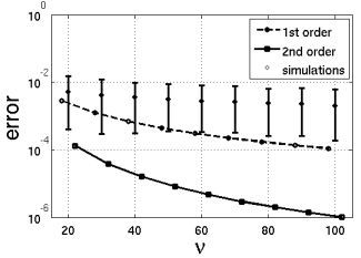
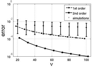
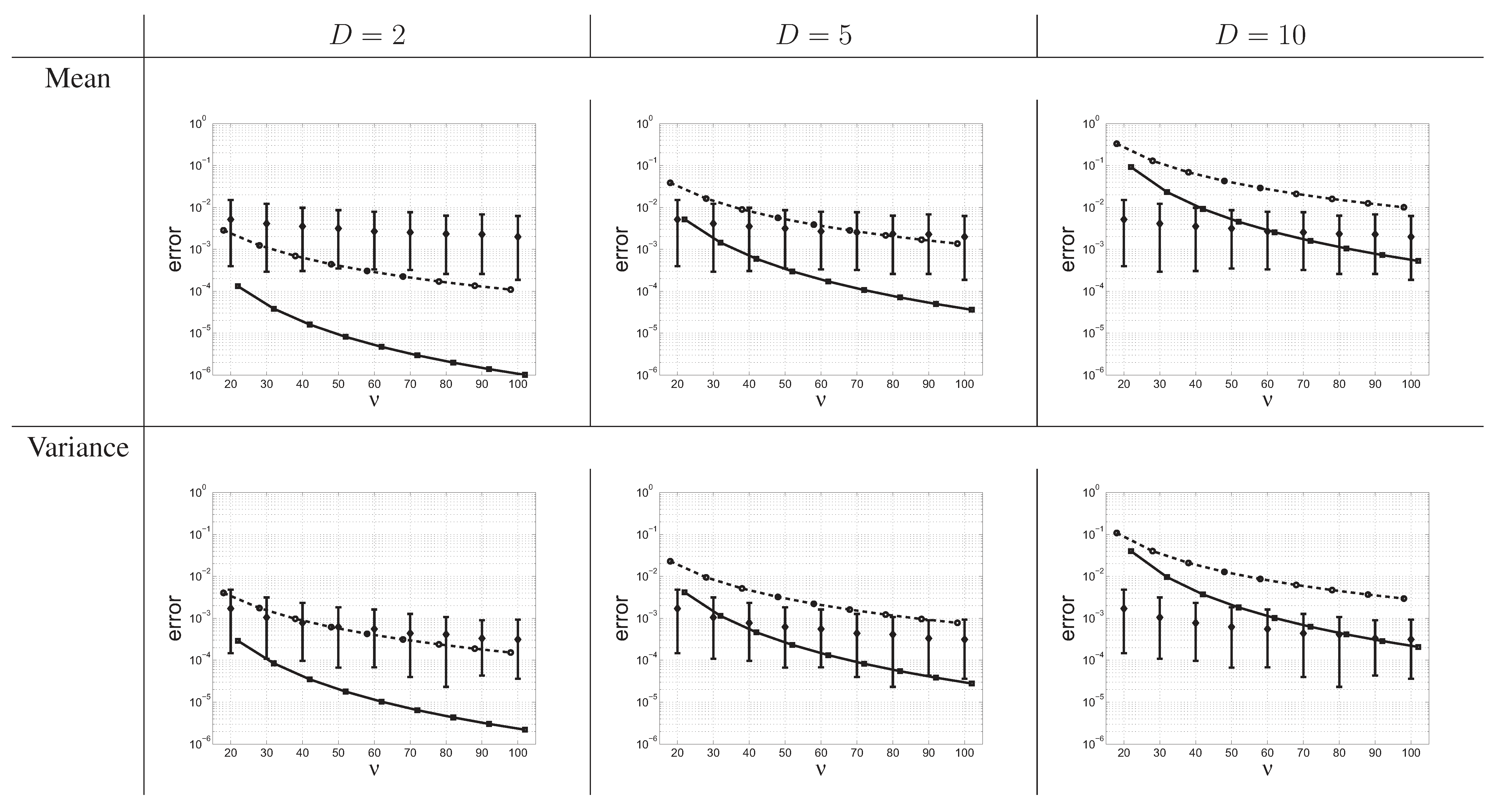
5. Simulation Study

We conducted the following computations for $D\in \{2,5,10\}$. To assess the accuracy of the asymptotic expansion of the cumulants of sample entropy, we calculated the error made by the first and second central moments (i.e., the mean and variance of the distribution) compared to the exact values as a function of ν. As a way of comparison, we computed the same quantities for 500 different homogeneous positive definite matrices Σ (i.e., with all non-diagonal elements equal to the same value ρ, generated uniformly); for each value of Σ and ν, we generated 1,000 samples from $S\sim \mathrm{Wishart}(\nu ,\Sigma )$, computed the corresponding values of sample entropy, and approximated the moments by the corresponding sampling moments. The results are reported in Figure 1.

6. Discussion

In this work, we calculated both the moments of $\left|S\right|/|\nu \Sigma |$ and the cumulant-generating function of $U=-ln\left(\right|S|/|\nu \Sigma \left|\right)$ when S is Wishart distributed with ν degrees of freedom and scale matrix Σ. From there, we provided an asymptotic approximation of the first four central moments of U. We also proved that U is asymptotically normally distributed. We then demonstrated the quality of the normal approximation compared to simulations. We finally applied these results to the multivariate normal distribution to provide asymptotic approximations of the sample and posterior distributions of differential entropy, as well as an asymptotic approximation of the sample and posterior mean of multiinformation.

Interestingly, the moments of $\left|S\right|/|\nu \Sigma |$ and, as a way of consequence, the cumulant-generating function of U depends on the distribution that S follows only through the matrix dimension D and the degree of freedom ν, but not through Σ. This means that the exact distribution of U is also independent from that parameter and could possibly be tabulated as a function of the two integer parameters.

As mentioned in the introduction, the sample differential entropy defined in Equation (1) is equal to the plug-in estimator for differential entropy. The present work provides a quantification in the case of multivariate normal samples for the well-known negative bias for this estimator [7]. Obviously, Equation (18) confirms that, to correct from this bias, one must take the uniformly minimum variance unbiased (UMVU) estimator [1].

The posterior derivation that we presented here is a particular case of the Bayesian posterior estimate obtained by [3] with, in our case, the prior distribution for Σ taken as Jeffreys prior (i.e., $q=-1$ and $B=0$ with their notations). While the same analysis as in [3] could have been performed, it would essentially lead to the same result, since we only consider the asymptotic case, where the sample is large and the prior distribution is supposed to have very little influence—provided that it does not contradict the data. The present study also shows an interesting feature of Bayesian estimation with respect to the above-mentioned negative bias. As the sample differential entropy tends to underestimate $H(\Sigma )$ by a factor of $m/2$, if one takes the posterior mean as the Bayesian estimate of $H(\Sigma )$, then the negative bias is corrected by the opposite factor.

Figure 1. Error on the mean (top row) and variance (bottom row) of sample entropy for various values of D and ν when using the first-order approximation (circles), the second-order approximation (squares), or the sampling scheme (diamonds). The error was calculated as the absolute value of the difference between the approximation and the true value. For the sampling scheme are represented the median as well as the symmetrical 90% probability interval of the error. Scale on y axis is logarithmic.

Figure 1. Error on the mean (top row) and variance (bottom row) of sample entropy for various values of D and ν when using the first-order approximation (circles), the second-order approximation (squares), or the sampling scheme (diamonds). The error was calculated as the absolute value of the difference between the approximation and the true value. For the sampling scheme are represented the median as well as the symmetrical 90% probability interval of the error. Scale on y axis is logarithmic.

We were also able to obtain an asymptotic approximation of the sampling and posterior expectations of mutual information and multiinformation. Contrary to the general argument developed by [7], we proved that, for multivariate normal distributions, the negative bias for differential entropy does entail a positive bias for mutual information. This result is in agreement with the fact that, under the null hypothesis of Σ diagonal matrix, corresponding to $i(\Sigma )=0$, $\nu i(S/\nu )$ is asymptotically chi square distributed with ${\sum }_{i<j}{D}_i{D}_j/2$ degrees of freedom and, hence, has an expectation equal to that value [19] (pp. 306–307). Surprisingly, and unlike what was said for entropy, the positive bias of the sample multiinformation was not corrected by the Bayesian approach. A naive correction of minus the positive bias could lead to negative values, which is impossible by construction of multiinformation. Note that, using the present results alone, we were not able to obtain an asymptotic approximation for the variance of the same measures.

In the present paper, we used loose versions of the inequalities proposed in [20] to prove the monotonicity and sign of the cumulants of U (see Section 2.1 and Appendix). Note that, using the same inequalities, it seems that it would also be possible to obtain lower and upper bounds for these quantities, instead of asymptotic approximations. These bounds would be useful complements to the approximations provided in the present manuscript.

References

- Ahmed, N.A.; Gokhale, D.V. Entropy expressions and their estimators for multivariate distributions. IEEE Trans. Inform. Theory 1989, 35, 688–692. [Google Scholar] [CrossRef]
- Misra, N.; Singh, H.; Demchuk, E. Estimation of the entropy of a multivariate normal distribution. J. Multivariate Anal. 2005, 92, 324–342. [Google Scholar] [CrossRef]
- Gupta, M.; Srivastava, S. Parametric Bayesian estimation od differential entropy and relative entropy. Entropy 2010, 12, 818–843. [Google Scholar] [CrossRef]
- Beirlant, J.; Dudewicz, E.J.; Györfi, L.; van der Meulen, E.C. Nonparametric entropy estimation: An overview. Int. J. Math. Stastist. Sci. 1997, 6, 17–39. [Google Scholar]
- Strong, S.P.; Koberle, R.; de Ruyter van Steveninck, R.R.; Bialek, W. Entropy and information in neural spike trains. Phys. Rev. Lett. 1998, 80, 197–200. [Google Scholar] [CrossRef]
- Antos, A.; Kontoyiannis, I. Convergence properties of functional estimates for discrete distributions. Random Struct. Algor. 2001, 19, 163–193. [Google Scholar] [CrossRef]
- Paninski, L. Estimation of entropy and mutual information. Neural Comput. 2003, 15, 1191–1253. [Google Scholar] [CrossRef]
- Wolpert, D.H.; Wolf, D.R. Estimating functions of probability distributions from a finite set of samples. Phys. Rev. E 1995, 52, 6841–6854. [Google Scholar] [CrossRef]
- Wolpert, D.H.; Wolf, D.R. Erratum: Estimating functions of probability distributions from a finite set of samples. Phys. Rev. E 1996, 54, 6973. [Google Scholar] [CrossRef]
- Anderson, T.W. An Introduction to Multivariate Statistical Analysis; John Wiley and Sons: New York, NY, USA, 1958. [Google Scholar]
- Abramowitz, M.; Stegun, I.A. Handbook of Mathematical Functions; Applied Mathematics Series 55; National Bureau of Standards: Washington, DC, USA, 1972. [Google Scholar]
- Anderson, T.W. An Introduction to Multivariate Statistical Analysis, 3rd ed.; Series in Probability and Mathematical Statistics; John Wiley and Sons: New York, NY, USA, 2003. [Google Scholar]
- Gelman, A.; Carlin, J.B.; Stern, H.S.; Rubin, D.B. Bayesian Data Analysis; Texts in Statistical Science; Chapman & Hall: London, UK, 1998. [Google Scholar]
- Watanabe, S. Information theoretical analysis of multivariate correlation. IBM J. Res. Dev. 1960, 4, 66–82. [Google Scholar] [CrossRef]
- Garner, W.R. Uncertainty and Structure as Psychological Concepts; John Wiley & Sons: New York, NY, USA, 1962. [Google Scholar]
- Joe, H. Relative entropy measures of multivariate dependence. J. Am. Statist. Assoc. 1989, 84, 157–164. [Google Scholar] [CrossRef]
- Studený, M.; Vejnarová, J. The multiinformation function as a tool for measuring stochastic dependence. In Proceedings of the NATO Advanced Study Institute on Learning in Graphical Models; Jordan, M.I., Ed.; MIT Press: Cambridge, MA, USA, 1998; pp. 261–298. [Google Scholar]
- Press, S.J. Applied Multivariate Analysis. Using Bayesian and Frequentist Methods of Inference, 2nd ed.; Dover: Mineola, NY, USA, 2005. [Google Scholar]
- Kullback, S. Information Theory and Statistics; Dover: Mineola, NY, USA, 1968. [Google Scholar]
- Chen, C.P. Inequalities for the polygamma functions with application. Gener. Math. 2005, 13, 65–72. [Google Scholar]
Appendix
1. Results for
2. Results for ,
© 2011 by the authors; licensee MDPI, Basel, Switzerland. This article is an open access article distributed under the terms and conditions of the Creative Commons Attribution license (http://creativecommons.org/licenses/by/3.0/).
Share and Cite
Marrelec, G.; Benali, H. Large-Sample Asymptotic Approximations for the Sampling and Posterior Distributions of Differential Entropy for Multivariate Normal Distributions. Entropy 2011, 13, 805-819. https://doi.org/10.3390/e13040805
Marrelec G, Benali H. Large-Sample Asymptotic Approximations for the Sampling and Posterior Distributions of Differential Entropy for Multivariate Normal Distributions. Entropy. 2011; 13(4):805-819. https://doi.org/10.3390/e13040805
Chicago/Turabian StyleMarrelec, Guillaume, and Habib Benali. 2011. "Large-Sample Asymptotic Approximations for the Sampling and Posterior Distributions of Differential Entropy for Multivariate Normal Distributions" Entropy 13, no. 4: 805-819. https://doi.org/10.3390/e13040805