Article

A Feature Subset Selection Method Based On High-Dimensional Mutual Information

1
Institute of Developmental Biology and Molecular Medicine, Fudan University, 220 Handan Road, Shanghai 200433, China
2
School of Life Sciences, Fudan University, 220 Handan Road, Shanghai 200433, China
3
School of Computer Engineering, Nanyang Technological University, 50 Nanyang Avenue, 639798, Singapore
*
Authors to whom correspondence should be addressed.
Entropy 2011, 13(4), 860-901; https://doi.org/10.3390/e13040860
Submission received: 8 January 2011 / Revised: 18 March 2011 / Accepted: 23 March 2011 / Published: 19 April 2011

Abstract

:
Feature selection is an important step in building accurate classifiers and provides better understanding of the data sets. In this paper, we propose a feature subset selection method based on high-dimensional mutual information. We also propose to use the entropy of the class attribute as a criterion to determine the appropriate subset of features when building classifiers. We prove that if the mutual information between a feature set X and the class attribute Y equals to the entropy of Y, then X is a Markov Blanket of Y. We show that in some cases, it is infeasible to approximate the high-dimensional mutual information with algebraic combinations of pairwise mutual information in any forms. In addition, the exhaustive searches of all combinations of features are prerequisite for finding the optimal feature subsets for classifying these kinds of data sets. We show that our approach outperforms existing filter feature subset selection methods for most of the 24 selected benchmark data sets.

1. Introduction

In solving classification problems, many induction algorithms suffer from the curse of dimensionality [1]. The inclusion of irrelevant, redundant and noisy attributes in the model building phase can also result in poor predictive performance and increased computation [2]. Feature selection is critical to overcome the over-fitting problems by finding the informative and discriminatory features, to improve the performance of classification algorithm, and to avoid the curse of dimensionality.
Recently, some methods have been proposed to select feature subsets with mutual information (MI) [3,4,5,6,7,8,9,10,11,12,13]. Because it is expensive to evaluate MI between continuous features and the class attribute, some studies [3,7,8,9,10,12] use approximation methods to estimate MI of continuous features. Even for discrete features, it is very difficult to compute high dimensional MI [7]. Hence, in [3,4,5,6,7,8,9,11,12,13], the high dimensional MI is replaced with the algebraic combinations of two dimensional MIs to accelerate the computation. In particular, Peng et al. [7] proposed a theorem that for the first-order incremental search (greedy search, forward search), mRMR (minimal redundancy maximal relevance) is equivalent to Max-Dependency, i.e., maximal high dimensional MI.
In this paper, we introduce the Discrete Function Learning algorithm [14] as a filter feature selection method, using high-dimensional mutual information to measure the relationship between the candidate feature subsets, X , and the class attribute, Y. In our method, we propose to use the entropy of the class attribute as the criterion to choose the appropriate number of features, instead of subjectively assigning the number of features in prior. Specifically, we prove that if the mutual information between a feature set X and the class attribute Y equals to the entropy of Y, then X is a Markov Blanket of Y. The DFL algorithm uses a unique searching schema, which is greedy in its first round of searching and still guarantees the exhaustive searching of all combinations of features in the searching space. Accordingly, the DFL algorithm has the average complexity of O ( k · n · ( N + log n ) ) and the worst case complexity of O ( ( N + log n ) · n K ) , respectively. Due to the merit of this searching schema and using the entropy of class attribute as the stopping criterion in evaluating features subsets, the DFL algorithm can solve some special problems that cannot be solved by existing feature selection methods based on pairwise mutual information. We also demonstrate that in these cases, the high-dimensional mutual information cannot be replaced with algebraic combinations of pairwise mutual information.
To evaluate the performance of the DFL algorithm, we choose 24 benchmark data sets from the classic UCI machine learning repository [15] and high-dimensional gene (or protein) expression profiles in [16,17,18,19], whose numbers of features range from 4 to 15454. We compare our method with two filter feature subset selection method, CFS (Correlation-based Feature Selection) [20] and CSE (Consistency-based Subset Evaluation) [21], and the Wrapper Subset Evaluation (WSE) [22] method. Experimental results show that our method outperforms the CFS and CSE methods in most data sets selected. The accuracies from our method and the WSE method are comparable, but our method has much better efficiency than the WSE method has.
The rest of the paper is organized as follows. In Section 2, we review existing feature selection methods and analyze their limitations. Section 3. will reintroduce the Discrete Function Learning (DFL) algorithm, discuss its relationship with the Markov Blanket, and analyze its complexity and correctness. Then, we introduce the ϵ value method for noisy data sets in Section 4. Next, we discuss how to choose parameters of the DFL algorithm in Section 5. The prediction method is introduced in Section 6. Section 7 will discuss two critical issues in implementation. Experimental results are discussed in Section 8. We further show that the it is infeasible in some situations to replace high-dimensional mutual information with algebraic combinations of pairwise ones in Section 9. Finally, Section 10 summarizes this paper.

2. Related Work

In this section, we review current feature selection methods, and discuss their limitations. First, we categorize current feature selection methods. Then, we specifically describe feature selection methods based on information theory. Finally, we analyze the shortcomings of them.

2.1. Categorization of Feature Selection Methods

Feature selection methods fall into two main categories, those evaluating individual features and those evaluating subsets of features.
In the individual feature selection methods, a certain evaluation statistic is calculated for each feature, then a ranked feature list is provided in a predefined order of the statistic. The statistics used for individual feature selection include information gain [2,23,24], signal-to-noise (S2N) statistic [16,17,18,25], correlation coefficient [26], t-statistic [23], χ 2 -statistic [23,27] and others. The main shortcoming of these individual feature selection methods lies in that a larger than necessary number of redundant top features with similar value patterns, like gene expression patterns, are selected to build the models. Hence, these approaches often bring much redundancy to the models, since the selected features carry similar information about the class attribute. According to the principle of Occam’s razor, these models are not optimal although accurate, since they are often complex and suffer from the risk of overfitting the training data sets [24]. In addition, the large number of features in the predictors makes it difficult to know which features are really useful for recognizing different classes.
In the feature subset selection methods, a search algorithm is often employed to find the optimal feature subsets. In evaluating a feature subset, a predefined score is calculated for the feature subset. Since the number of feature subsets grows exponentially with the number of features, heuristic searching algorithms, such as the forward greedy selection, are often employed to solve the problem. Examples of feature subset selection methods are CFS (Correlation-based Feature Selection) [20], CSE (Consistency-based Subset Evaluation) [21], and the WSE (Wrapper Subset Evaluation) [22]. Most feature subset selection methods use heuristic measures to evaluate feature subset under consideration, such as the CFS and CSE methods. The WSE method is inefficient, especially when dealing with high-dimensional data sets.
There is another popular way to categorize these algorithms as “filter” or “wrapper” methods [28]. While a filter is used independent of the classification algorithm, the wrapper is used with the classification algorithm when searching the optimal feature subsets [22].

2.2. Theoretic Background

The entropy of a discrete random variable X is defined in terms of probability of observing a particular value x of X as [29]:
H ( X ) = x P ( X = x ) log P ( X = x )
The entropy is used to describe the diversity of a variable or vector. The more diverse a variable or vector is, the larger entropy they will have. Generally, vectors are more diverse than individual variables, hence have larger entropy. Hereafter, for the purpose of simplicity, we represent P ( X = x ) with p ( x ) , P ( Y = y ) with p ( y ) , and so on. The MI between a vector X and Y is defined as [29]:
I ( X ; Y ) = H ( Y ) H ( Y | X ) = H ( X ) H ( X | Y ) = H ( X ) + H ( Y ) H ( X , Y )
Mutual information is always non-negative and can be used to measure the relation between two variable, a variable and a vector (Equation 2), or two vectors. Basically, the stronger the relation between two variables, the larger MI they will have. Zero MI means the two variables are independent or have no relation, which is formally given in Theorem 1. Proof of Theorem 1 can be found in [30].
Theorem 1
For any discrete random variables Y and Z, I ( Y ; Z ) 0 . Moreover, I ( Y ; Z ) = 0 if and only if Y and Z are independent.
The conditional MI I ( X ; Y | Z ) (the MI between X and Y given Z) [30] is defined by
I ( X ; Y | Z ) = H ( Y | Z ) H ( Y | X , Z ) = x , y , z p ( x , y , z ) p ( x , y | z ) p ( x | z ) p ( y | z )
The chain rule for MI is give by Theorem 2, for which the proof is available in [30].
Theorem 2
I ( X 1 , X 2 , , X n ; Y ) = i = 1 n I ( X i ; Y | X i 1 , X i 2 , , X 1 ) .

2.3. Feature Selection Methods Based on Information Theory

Let us review existing feature selection methods based on MI, which include work by Dumais et al. [31], Yang and Pedersen [32], Kwak and Choi [4], Vidal-Naquet and Ullman [5], Fleuret [6], Chow and Huang [33], Peng et al. [7], Bonev and Escolano [8], Cai et al. [9], Estevez et al. [11], Vinh et al. [13], Zhu et al. [10], and Sotoca and Pla [12]. These methods can also be classified into two categories.
In the first category, i.e., the individual feature selection methods, features are ranked according to their MI with the class label. Then, the first k features [31] or the features with a bigger MI than a predefined threshold value [32] are chosen.
The second category is feature subset selection. In this category, the forward selection searching algorithm, i.e., the greedy algorithm, is often used to find the predefined k features. In the first iteration, the feature X i which shares the largest MI with the class attribute Y is selected to the target feature subset U . Then, in the next step, the selection criterion is to determine how much information can be added with respect to the already existing X ( 1 ) . Therefore, the X ( 2 ) with maximum I ( X i , X ( 1 ) ; Y ) I ( X ( 1 ) ; Y ) is added to U [5]. Formally, the features X ( 1 ) , , X ( k ) are selected with the following criteria, X ( 1 ) = arg max i I ( X i ; Y ) and
X ( s ) = arg max X i P s 1 min X ( j ) U s 1 ( I ( X i , X ( j ) ; Y ) I ( X ( j ) ; Y ) )
where s , 1 < s k , i = 1 , , ( n s + 1 ) , j = 1 , , ( s 1 ) , and P s is the feature pool by removing X ( 1 ) , , X ( s ) , with P 1 = V X ( 1 ) , P s = P s 1 X ( s ) , and U s is the set of selected features, with U 1 = { X ( 1 ) } , U s = U s 1 { X ( s ) } .
From Theorem 2, we have I ( X i , X ( j ) ; Y ) = I ( X ( j ) ; Y ) + I ( X i ; Y | X ( j ) ) , then I ( X i ; Y | X ( j ) ) = I ( X i , X ( j ) ; Y ) I ( X ( j ) ; Y ) . Therefore, Equation 4 is equivalent to maximizing conditional MI, min X ( j ) U s 1 I ( X i ; Y | X ( j ) ) [6,9] in Equation 5.
X ( s ) = arg max X i P s 1 min X ( j ) U s 1 I ( X i ; Y | X ( j ) )
Battiti [3] introduced a heuristic algorithm to find the feature subsets, as in Equation 6. This method is similar to those in Equations 4 and 5 [5,6], i.e., but not theoretically formulated.
X ( s ) = arg max X i P s 1 [ I ( X i ; Y ) β X ( j ) U s 1 I ( X i ; X ( j ) ) ]
where β was a manually tuned parameter.
Kwak and Choi [4] introduced a modified version of Equation 6 as Equation 7.
X ( s ) = arg max X i P s 1 [ I ( X i ; Y ) β X ( j ) U s 1 I ( X ( j ) ; Y ) H ( X ( j ) ) I ( X i ; X ( j ) ) ]
similar to Equation 6, where β was a manually tuned parameter.
Chow and Huang [33] proposed an approximation method to evaluate MI between continuous features and the class attribute. Then, Chow and Huang [33] used the heuristic criteria, feature relevance criterion (FRC) and feature similarity criterion (FSC) in Equation 8 and 9 to choose features with a forward selection process.
F R C ( X i ) = I ( { U , X i } ; Y )
F S C ( X i ) = arg max X ( j ) U ( I ( X i ; X ( j ) ) H ( X ( j ) ) )
This method essentially finds the most relevant feature with maximal F R C ( X i ) , then evaluates its redundancy by calculating F S C ( X i ) with respect to the selected features individually. If F S C ( X i ) is larger than a predefined threshold value, it is considered as a redundant feature and will not be chosen [33].
Peng et al. [7] proposed to use X ( 1 ) = arg max i I ( X i ; Y ) and Equation 10 to choose a new feature.
X ( s ) = arg max X i P s 1 [ I ( X i ; Y ) 1 s 1 X ( j ) U s 1 I ( X i ; X ( j ) ) ]
Peng et al. [7] also used an approximation method to calculate the MI between continuous features and the class attribute.
Later, Estevez et al. [11] proposed a variant of Equation 10 in Equation 11.
X ( s ) = arg max X i P s 1 [ I ( X i ; Y ) 1 s 1 X ( j ) U s 1 I ^ ( X i ; X ( j ) ) ]
where I ^ ( X i ; X ( j ) ) was the normalized mutual information defined in Equation 12.
I ^ ( X i ; X ( j ) ) = I ( X i ; X ( j ) ) m i n ( H ( X i ) , H ( X ( j ) ) )
Vinh et al. [13] recently further proposed to improve Equation 11 with Equation 13.
X ( s ) = arg max X i P s 1 [ I ^ ( X i ; Y ) 1 s 1 X ( j ) U s 1 I ^ ( X i ; X ( j ) ) ]
where I ^ ( X i ; Y ) was defined similarly as Equation 12.
Recently, Sotoca and Pla [12] proposed a method to perform clustering of features based on conditional mutual information, then a representative feature of each cluster was chosen as a selected feature. Maji [34] also proposed clustering method for choosing features according to some measures derived from mutual information.

2.4. Limitations of Current Feature Subset Selection Methods

For most existing feature subset selection methods based on MI, one common major shortcoming is that the candidate feature is pairwise evaluated with respect to every individual feature in the selected feature subset U s 1 step by step. The motivation underlying Equation 4 and 5 is that X i is good only if it carries information about Y, and if this information has not been caught by any of the X ( j ) already picked [6]. However, it is unknown whether the existing features as a vector have captured the information carried by X i or not. Another shortcoming is that it needs to specify the number of features k in prior. As shown in [1,4,7,8,10,11,13,33], the performances of existing algorithms applied to the selected features were sensitive to the predefined k. In addition, it also introduces some redundant computation when evaluating the new feature X i with respect to each of the already picked features X ( j ) U s 1 , which will be discussed further in Section 9.

3. The Discrete Function Learning Algorithm

3.1. Theoretic Motivation and Foundation

We restate the theorem about the relationship between the MI I ( X ; Y ) and the number of attributes in X .
Theorem 3 ([35], p. 26)
I ( { X , Z } ; Y ) I ( X ; Y ) , with equality if and only if p ( y | x ) = p ( y | x , z ) for all ( x , y , z ) with p ( x , y , z ) > 0 .
Proof of Theorem 3 can be found in [35]. In Theorem 3, it can be seen that { X , Z } will contain more or equal information about Y as X does. To put it another way, the more variables, the more information is provided about another variable.
To measure which subset of features is optimal, we reformulate the following theorem, which is the theoretical foundation of our algorithm.
Theorem 4
If the MI between X and Y is equal to the entropy of Y, i.e., I ( X ; Y ) = H ( Y ) , then Y is a function of X .
It has been proved that if H ( Y | X ) = 0 , then Y is a function of X [30]. Since I ( X ; Y ) = H ( X ) H ( Y | X ) , it is immediate to obtain Theorem 4. The entropy H ( Y ) represents the diversity of the variable Y. The MI I ( X ; Y ) represents the dependence between vector X and Y. From this point of view, Theorem 4 actually says that the dependence between vector X and Y is very strong, such that there is no more diversity for Y if X has been known. In other words, the value of X can fully determine the value of Y. X satisfying Theorem 4 is defined as essential attributes (EAs), because X essentially determines the value of Y [14].

3.2. Performing Feature Selection

The feature selection is often used as a preprocessing step before building models for classification. The aim of feature selection is to remove the irrelevant and redundant features, so that the induction algorithms can produce better prediction accuracies with more concise models and better efficiency.
From Theorem 1, the irrelevant features tend to share zero or very small MI with the class attribute in the presence of noise. Therefore, the irrelevant features can be eliminated by choosing those features with relatively large MI with the class attribute in modelling process.
When choosing candidate features, our approach maximizes the MI between the feature subsets and the class attribute. Suppose that U s 1 has already been selected at the step s 1 , and the DFL algorithm is trying to add a new feature X i V U s 1 to U s 1 . Specifically, our method uses the following criterion, X ( 1 ) = arg max i I ( X i ; Y ) and
X ( s ) = arg max i I ( U s 1 , X i ; Y )
where s , 1 < s k , U 1 = { X ( 1 ) } , and U s = U s 1 { X ( s ) } . From Equation 14, it is obvious that the irrelevant features have lost the opportunity to be chosen as EAs of the classifiers after the first EA, X ( 1 ) , is chosen, since I ( X i ; Y ) is very small if X i is an irrelevant feature.
Next, we illustrate how to eliminate the redundant features. From Theorem 2, we have
I ( U s 1 , X i ; Y ) = I ( U s 1 ; Y ) + I ( X i ; Y | U s 1 )
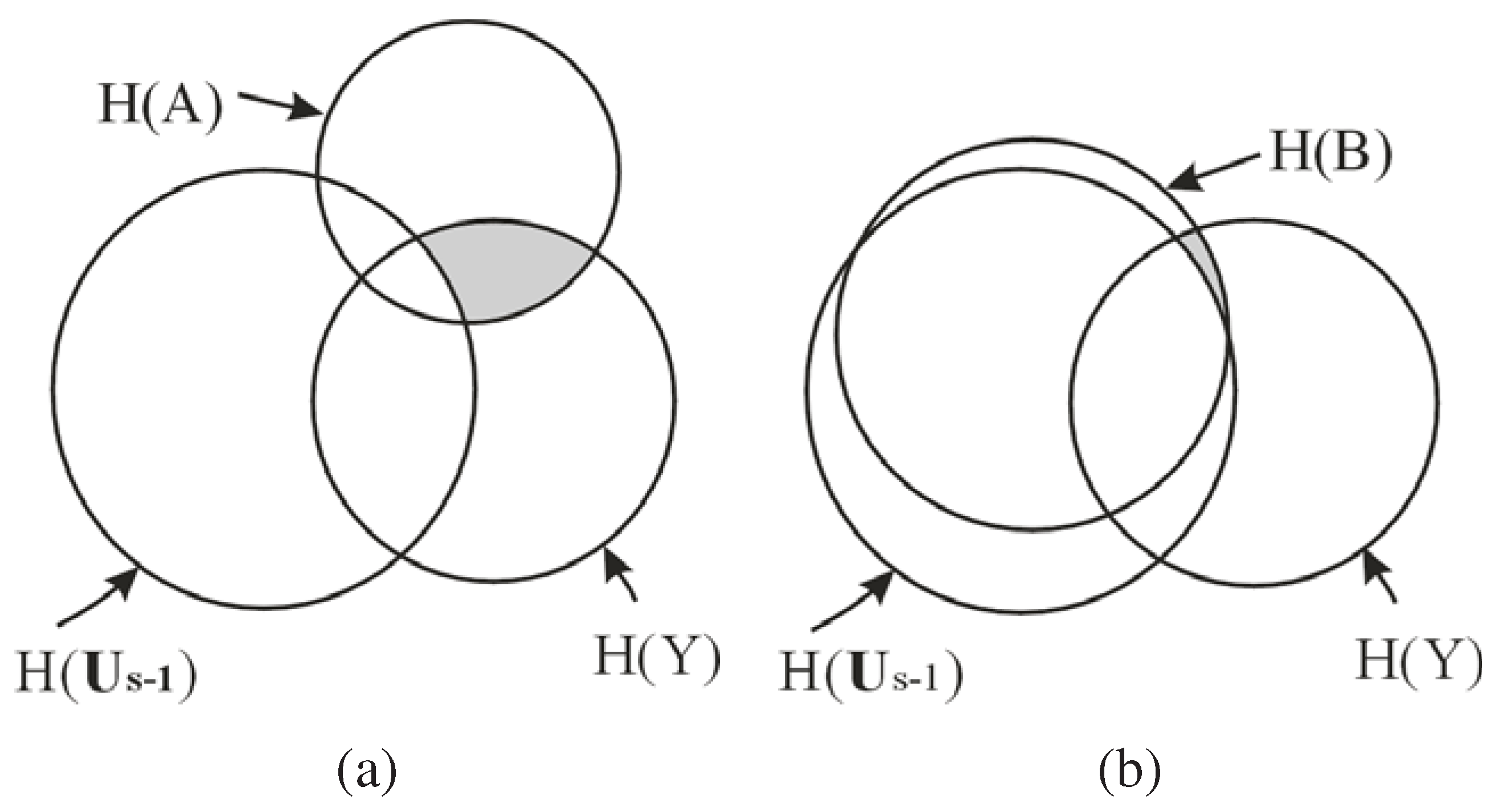
In Equation 15, note that I ( U s 1 ; Y ) does not change when trying different X i V U s 1 . Hence, the maximization of I ( U s 1 , X i ; Y ) in our method is actually maximizing I ( X i ; Y | U s 1 ) , as shown by the shaded region in Figure 1, which is the conditional MI of X i and Y given the already selected features U s 1 , i.e., the information of Y not captured by U s 1 but carried by X i . As shown in Figure 1 (b), if the new feature B is a redundant feature, i.e., I ( U s 1 ; B ) is large, then the additional information of Y carried by X i , I ( B ; Y | U s 1 ) , will be small. Consequently, B is unlikely to be chosen as an EA based on Equation 15. Hence, the redundant features are automatically eliminated by maximizing I ( U s 1 , X i ; Y ) .
From Theorem 4, if a feature subset U V satisfies I ( U ; Y ) = H ( Y ) , then Y is a deterministic function of U , which means that U is a complete and optimal feature subset. But the real data sets are often noisy. Thus, the DFL algorithm estimates the optimal feature subsets with the ϵ value method to be introduced in Section 4. by finding feature subsets to satisfy H ( Y ) I ( U ; Y ) ϵ × H ( Y ) .
In summary, the irrelevant and redundant features can be automatically removed, if the new candidate feature X i is evaluated with respect to the selected features as a vector U s 1 by maximizing I ( U s 1 , X i ; Y ) . Furthermore, the optimal subset of features can be determined by evaluating I ( U ; Y ) with respect to H ( Y ) .

3.3. Relation to Markov Blanket

Conditional Independence (see [36], p. 83) is a concept used in graphical models, especially Bayesian networks [36].
Definition 1 (Conditional Independence)
Let V = { X 1 , , X n } and P ( · ) be a joint probability function over the variables in V . X , Y , and Z V , the sets Y and Z are said to be conditional independent given X if
P ( Y | X , Z ) = P ( Y | X )
In other words, learning the value of Z does not provide additional information about Y , once we know X .
Markov Blanket [36] is defined as follows.
Definition 2 (Markov Blanket)
Let U be some set of features(variables) which does not contain X i . We say that U is a Markov Blanket for X i if X i is conditional independent of R = V { U { X i } } [37] given U , i.e.,
p ( x i | r , u ) = p ( x i | u ) , p ( r , u ) > 0
A set is called a Markov boundary of X i , if it is a minimum Markov Blanket of X i , i.e., none of its proper subsets satisfy Equation 17 (see [36], p. 97).
From the definition of Markov Blanket, it is known that if we can find a Markov Blanket U for the class attribute Y, then all other variables in V will be statistically independent of Y given U . This means that all the information that may influence the value of Y is stored in values of U [38]. In other words, Markov Blanket U has prevented other nodes from affecting the value of Y. Markov Blanket U also corresponds to strongly relevant features [39], as defined by Kohavi and John [22]. Therefore, if we can find a Markov Blanket U of Y as the candidate feature subsets, U should be the theoretical optimal subset of features to predict the value of Y, as discussed in [1,39].
Next, let us discuss the relationship between our method and Markov Blanket. First, we restate Theorem 5 and 6, which is needed to prove Theorem 7.
Theorem 5 ([40], p. 36)
Suppose that X is a set of discrete random variables, and Y are a finite discrete random variables. Then, m i n ( H ( X ) , H ( Y ) ) I ( X ; Y ) 0 .
Theorem 6 ([30], p. 43)
If Y = f ( X ) , where X is a set of discrete random variables, then H ( X ) H ( Y ) .
Theorem 7
If I ( X ; Y ) = H ( Y ) , X = { X ( 1 ) , , X ( k ) } V , Z V X , Y and Z are conditional independent given X .
Proof 1
Let us consider I ( X , Z ; Y ) , Z V X . Firstly,
H ( X , Z ) = H ( X ) + H ( Z | X ) H ( X )
Secondly, from Theorem 4, Y = f ( X ) . Then, from Theorem 6, H ( X ) H ( Y ) . So, H ( X , Z ) H ( X ) H ( Y ) Thus, m i n ( H ( X , Z ) , H ( Y ) ) = H ( Y ) . From Theorem 5, we have
I ( X , Z ; Y ) m i n ( H ( X , Z ) , H ( Y ) ) = H ( Y ) = I ( X ; Y )
On the other hand, from Theorem 3, we get
I ( X , Z ; Y ) I ( X ; Y )
From both Equation 18 and Equation 19, we obtain I ( X , Z ; Y ) = I ( X ; Y ) . Again from Theorem 3, we get p ( y | x , z ) = p ( y | x ) . That is to say, Y and Z are conditional independent given X .
Based on Theorem 7 and the concept of Markov Blanket, it is known that if I ( X ; Y ) = H ( Y ) , then X is a Markov Blanket of Y. Formally, we have
Theorem 8
If I ( X ; Y ) = H ( Y ) , then X is a Markov Blanket of Y.
Proof 2
Immediately from Theorem 7 and Definition 2.
As to be introduced in Section 4., I ( X ; Y ) = H ( Y ) can be satisfied only when the data sets are noiseless. However, with the introduction of ϵ method in Section 4., the set that carries most information of Y, H ( Y ) , is still a good estimation of the true Markov Blanket of Y. In addition, our method has competitive expected computational costs when compared to other methods for finding Markov Blankets, such as in [1,39,41,42].

3.4. The Discrete Function Learning Algorithm

U satisfying I ( U ; Y ) = H ( Y ) is a complete feature subsets in predicting Y based on Theorem 4. As also proved in Theorem 8, U satisfying I ( U ; Y ) = H ( Y ) is a good feature subsets for predicting Y. Thus, we aim to find U V with I ( U ; Y ) = H ( Y ) from the training data sets for solving the problem of finding optimal feature subsets.
For n discrete variables, there are totally 2 n subsets. Clearly, it is NP-hard to examine all possible subsets exhaustively. It is often the case that there are some irrelevant and redundant features in the domain V . Therefore, it is reasonable to reduce the searching space by only checking feature subsets with a predefined number of features. In this way, the problem can be solved in polynomial time.
Based on the above consideration, the DFL algorithm uses a parameter, the expected cardinality of EAs K, to prevent the exhaustive searching of all subsets of attributes by checking those subsets with fewer than or equal to K attributes, as listed in Table 1 and Table 2. The DFL algorithm has another parameter, the ϵ value, which will be elaborated in Section 4.
When trying to find the EAs from all combinations whose cardinalities are not larger than K, the DFL algorithm will examine the MI between the combination of variables under consideration, U , and the class attribute, Y. If I ( U ; Y ) = H ( Y ) , then the DFL algorithm will terminate its searching process, and obtain the classifiers by deleting the non-essential attributes and duplicate instances of the EAs in the training data sets, which corresponds to step 5 in Table 2. Meanwhile, the counts of different instances of ( U , Y ) are stored in the classifiers and will be used in the prediction process. In the algorithm, we use the following definitions.
Definition 3 (δ Superset)
Let X be a subset of V = { X 1 , X 2 , , X n } , then δ i ( X ) of X is a superset of X so that X δ i ( X ) and | δ i ( X ) | = | X | + i .
Definition 4 (Δ Supersets)
Let X be a subset of V = { X 1 , X 2 , , X n } , then Δ i ( X ) of X is the collective of all δ i ( X ) and Δ i ( X ) = δ i ( X ) .
Definition 5 (Searching Layer L of V )
Let X V , then the ith layer L i of all subsets of V is, | X | = i , L i = X .
Definition 6 (Searching Space)
The searching space of functions with a bounded indegree K is S K = i = 1 K L i .
From Definition 5, it is known that there are n i subsets of V in L i . And there are i = 1 K n i n K subsets of V in S K .
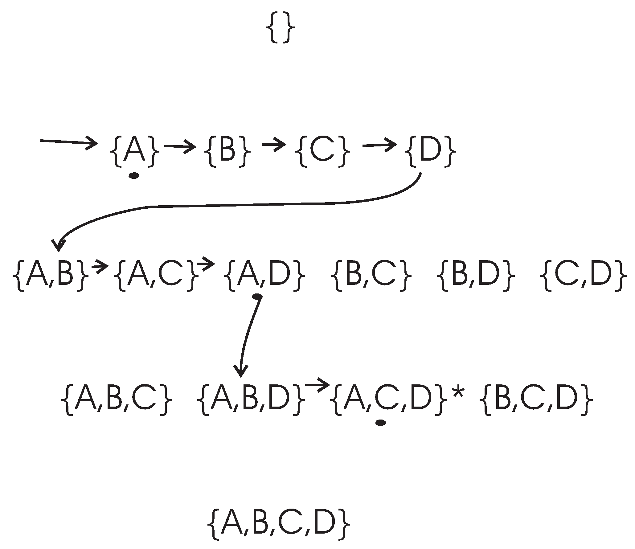
To clarify the search process of the DFL algorithm, let us consider an example, as shown in Figure 2. In this example, the set of attributes is V = { A , B , C , D } and the class attribute is determined with Y = ( A · C ) + ( A · D ) , where “·" and “+" are logic AND and OR operation respectively. The expected cardinality K is set to n = 4 for this example. However, there are only three real relevant features. We use k to represent the actual cardinality of the EAs, therefore, k = 3 in this example. The training data set T of this example is shown in Table 3.
The search procedure of the DFL algorithm for this example is shown in Figure 2. In the learning process, the DFL algorithm uses a data structure called Δ T r e e to store the Δ supersets in the searching process. For instance, the Δ T r e e when the DFL algorithm is learning the Y is shown in Figure 3.
As shown in Figure 2 and Figure 3, the DFL algorithm searches the first layer L 1 , then it sorts all subsets according to their MI with Y on L 1 . Consequently, the DFL algorithm finds that { A } shares the largest MI with Y among subsets on L 1 .
Next, the Δ 1 ( A ) s are added to the second layer of Δ T r e e , as shown in Figure 3. Similarly to L 1 , the DFL algorithm finds that { A , D } shares the largest mutual information with Y on L 2 . Then, the DFL algorithm searches through Δ 2 ( A ) , , Δ K 1 ( A ) , however it always decides the search order of Δ i + 1 ( A ) based on the calculation results of Δ i ( A ) . Finally, the DFL algorithm finds that the subset { A , C , D } satisfies the requirement of Theorem 4, i.e., I ( { A , C , D } ; Y ) = H ( Y ) , and will construct the function f for Y with these three attributes.
To determine f, firstly, B is deleted from training data set since it is a non-essential attribute. Then, the duplicate rows of ( { A , C , D } , Y ) are removed from the training data set to obtain the final function f as the truth table of ( A · C ) + ( A · D ) along with the counts for each instance of ( { A , C , D } , Y ) . This is the reason for which we name our algorithm as the Discrete Function Learning algorithm.
If the DFL algorithm still does not find the target subset, which satisfies the requirement of Theorem 4, in Kth layer L K , it will return to the first layer. Now, the first node on the L 1 and all its Δ 1 , , Δ K 1 supersets have already been checked. In the following, the DFL algorithm continues to calculate the second node on the first layer (and all its Δ 1 , , Δ K 1 supersets), the third one, and so on, until it reaches the end of L 1 and fulfills the exhaustive searching of S K .
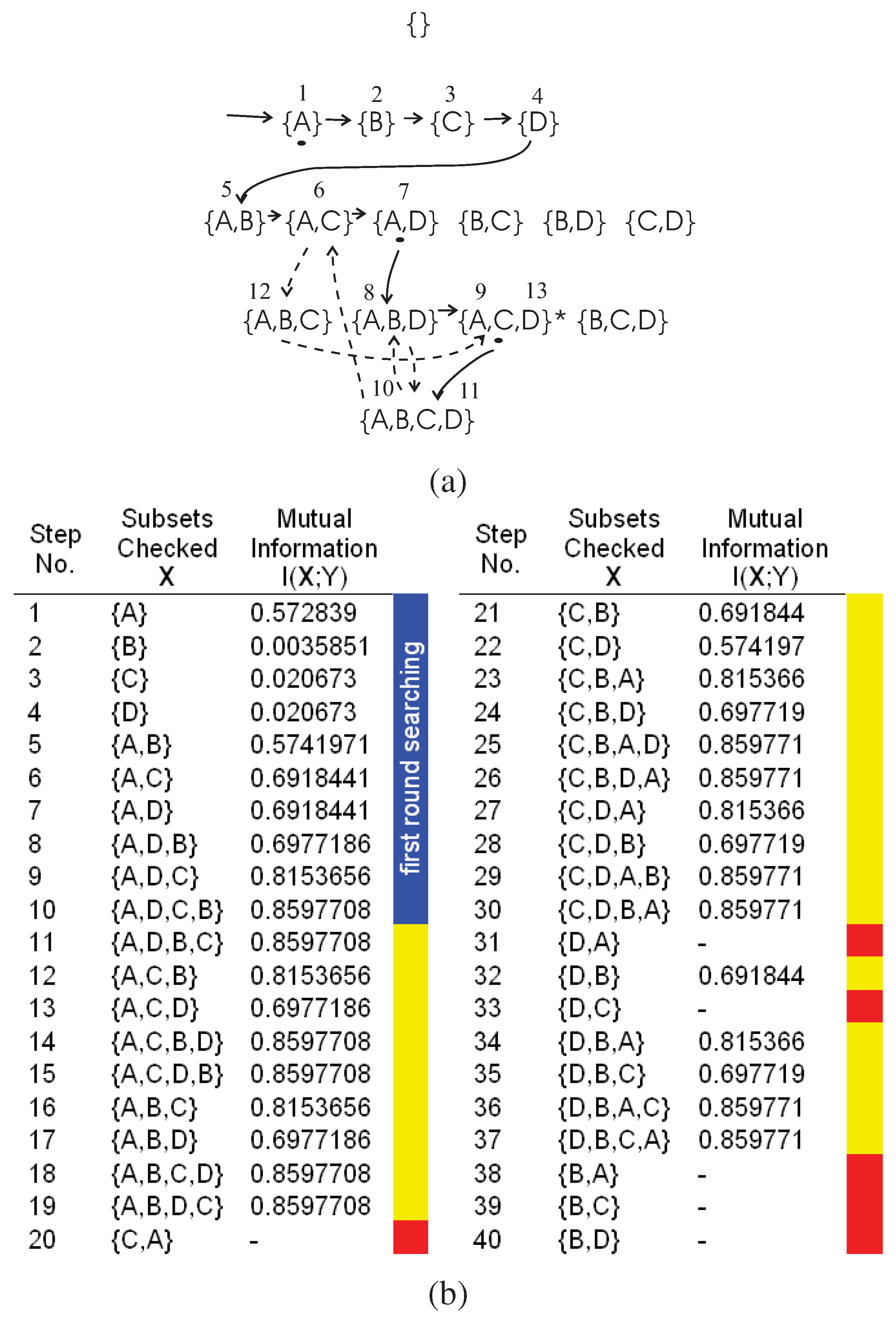
We use the example in Figure 4 to illustrate the searching steps beyond the first round searching of the DFL algorithm. Note that the DFL algorithm is the same as the classical greedy forward selection algorithm [43] and uses the mutual information I ( U ; Y ) as the greedy measure before it returns to the ( K 1 ) th layer from Kth layer for the first time. We name the searching steps before this first return as the first round searching of the DFL algorithm. As shown in Figure 4 (a) and (b), this first return happens after step 10.
To produce the exhaustive searching, we add one noisy sample (1100,1) to the training data set in Table 3. Then, we keep the same settings of K = 4 and ϵ = 0 . As shown in Figure 4 (b), the mutual information I ( X ; Y ) of all subsets is not equal to H ( Y ) = 0 . 977 . Therefore, the DFL algorithm will exhaustively check all subsets and finally report “Fail to identify the model for Y (the classifier) when ϵ = 0".
In Figure 4 (a), the first round searching is shown in the solid edges and the subsets checked in each step are shown in the blue region of Figure 4 (b). In Figure 4 (a), the dashed edges represent the searching path beyond the first round searching (only partly shown for the sake of legibility), marked as yellow regions in Figure 4 (b). The red regions are the subsets, as well as their supersets, that will not be checked after deploying the redundancy matrix to be introduced in Section B.1.

3.5. Complexity Analysis

First, we analyze the worst-case complexity of the DFL algorithm. As to be discussed in Section 7.1, the complexity to compute the MI I ( X , Y ) is O ( N ) , where N is the number of instances in the training data set. For the example in Figure 2, { A , B } will be visited twice from { A } and { B } in the worst case. { A , B , C } will be visited from { A , B } , { A , C } and { B , C } . Thus, { A , B , C } will be checked for 3 × 2 = 3 ! times in the worst case. In general, for a subset with K features, it will be checked for K ! times in the worst case. Hence, it takes O ( ( n 1 + n 2 2 ! + + n K K ! ) × N ) = O ( N · n K ) to examine all subsets in S K . Another computation intensive step is the sort step in line 7 of Table 2. In L 1 , there is only one sort operation, which takes O ( n log n ) time. In L 2 , there would be n sort operations, which takes O ( n 2 log n ) time. Similarly, in L K , the sort operation will be executed for n K 1 times, which takes O ( n K log n ) time. Therefore, the total complexity of the DFL algorithm is O ( ( N + log n ) · n K ) in the worst case.
Next, we analyze the expected complexity of the DFL algorithm. As described in Section 3.4, the actual cardinality of the EAs is k. After the EAs with k attributes are found in the subsets of cardinalities K , the DFL algorithm will stop its search. In our example, the K is 4, while the k is automatically determined as 3, since there are only 3 EAs in this example. Contributing to sort step in the line 7 of the subroutine, the algorithm makes the best choice on current layer of subsets. Since there are ( n 1 ) Δ 1 supersets for a given single element subset, ( n 2 ) Δ 1 supersets for a given two element subset, and so on. The DFL algorithm only considers i = 0 k 1 ( n i ) k · n subsets in the optimal case. Thus, the expected time complexity of the DFL algorithm is approximately O ( k · n · ( N + log n ) ) , where log n is for sort step in line 7 of Table 2.
Next, we consider the space complexity of the DFL algorithm. To store the information needed in the search processes, the DFL algorithm uses two data structures. The first one is a linked list, which stores the value list of every variable. Therefore, the space complexity of the first data structure is O ( N n ) . The second one is the Δ T r e e , which is a linked list of length K, and each node in the first dimension is itself a linked list. The Δ T r e e for the example in Figure 2 is shown in Figure 3. The first node of this data structure is used to store the single element subsets. If the DFL algorithm is processing { X i } and its Δ supersets, the second node to the Kth node are used to store Δ 1 to Δ K 1 [44] supersets of { X i } . If there are n variables, there would be i = 0 K 1 ( n i ) K n subsets in the Δ T r e e . To store the Δ T r e e , the space complexity would be O ( K n ) , since only the indexes of the variables are stored for each subsets. Therefore, the total space complexity of the DFL algorithm is O ( ( K + N ) · n ) .
Finally, we consider the sample complexity of the DFL algorithm. Akutsu et al. [45] proved that Ω ( 2 k + k l o g 2 n ) transition pairs are the theoretic lower bound to infer the Boolean networks, where n is the number of genes (variables), k is the maximum indegree of the genes, and a transition pair is ( { v ( t ) v ( t + 1 ) } ) (t is a time point). We further proved Theorem 9 when the genes have more than two discrete levels [46,47].
Theorem 9 ([46,47])
Ω ( b k + k l o g b n ) transition pairs are necessary in the worst case to identify the qualitative gene regulatory network models of maximum indegree k and the maximum number of discrete levels for variables b .
When considering the sample complexity in the context of feature selection (and classification), the transition pair should be replaced with { v , y } . Because k, n and b in the context of feature selection (classification) are the same as those in learning gene regulatory network models, the number of samples N in training data set T = { ( v i , y i ) : i = 1 , , N } has the same theoretic lower bound of Ω ( b k + k l o g b n ) as in Theorem 9.

3.6. Correctness Analysis

We first reintroduce Theorem 10, then show Theorem 11 about the correctness of the DFL algorithm.
Theorem 10 ([40], p. 37)
If Y = f ( X ) , then I ( X ; Y ) = H ( Y ) .
Theorem 11
Let V = { X 1 , , X n } . The DFL algorithm can find a consistent function Y = f ( U ) of maximum indegree K with O ( ( N + l o g n ) · n K ) time in the worse case from T = { ( v i , y i ) : i = 1 , 2 , , N } .
Proof 3
Since | X | = k , X is included in the searching space S K , where K k . Since Y = f ( X ) , I ( X ; Y ) = H ( Y ) based on Theorem 10. In the searching space S K , there exists at least one subset of V , i.e., X , which satisfies the criterion of Theorem 4.
Since the maximum indegree of the function is K k , the target subset U is included in the searching space S K . The DFL algorithm guarantees the check of all subsets in S K , which takes O ( N · n K ) time. The sort step in line 7 of Table 2 will be executed for O ( n K 1 ) times, which takes O ( n K · log n ) time. Finally, based on Theorem 4, the DFL algorithm will find a consistent function Y = f ( U ) in O ( ( N + log n ) · n K ) time in the worst case.
The word “consistent” means that the function Y = f ( U ) is consistent with the learning samples, i.e., u i , f ( u i ) = y i .

4. The ϵ Value Method for Noisy Data Sets

4.1. The ϵ Value Method

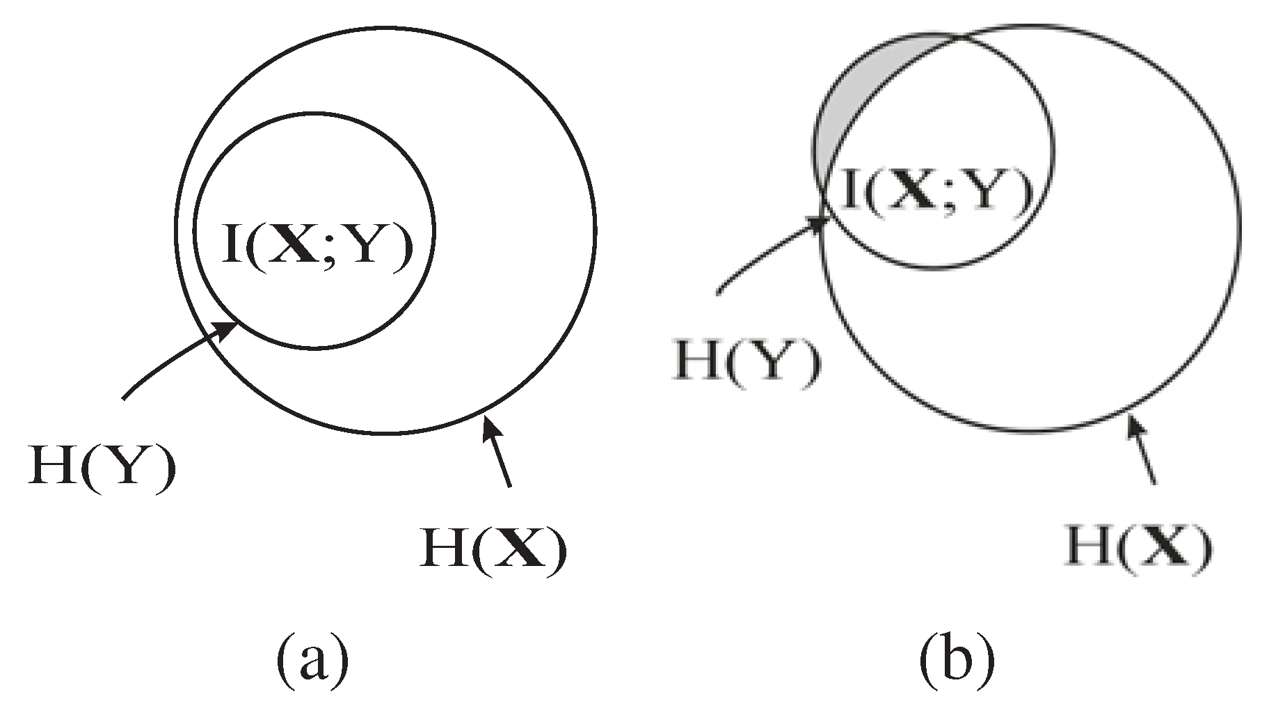
In Theorem 4, the exact functional relation demands the strict equality between the entropy of Y, H ( Y ) and the MI of X and Y, I ( X ; Y ) . However, this equality is often ruined by the noisy data, like microarray gene expression data. The noise changes the distribution of X or Y, therefore H ( X ) , H ( X , Y ) and H ( Y ) are changed due to the noise. From Equation 2, I ( X ; Y ) is changed as a consequence. In these cases, we have to relax the requirement to obtain the best estimated result. As shown in Figure 5, by defining a significance factor ϵ, if the difference between I ( X ; Y ) and H ( Y ) is less than ϵ × H ( Y ) , then the DFL algorithm will stop the searching process, and build the classifier for Y with X at the significant level ϵ.
Because H ( Y ) may be quite different for various classification problems, it is not appropriate to use an absolute value, like ϵ, to stop the searching process or not. Therefore, a percentage of H ( Y ) is used as the criterion to decide whether to stop the searching process or not.
The main idea of the ϵ value method is to find a subset of attributes which captures not all the diversity of the Y, H ( Y ) , but the major part of it, i.e., ( 1 ϵ ) × H ( Y ) , then to build functions with these attributes. The attributes in vectors showing strong dependence with Y are expected to be selected as input variables of Y, i.e., the EAs of the models, in the ϵ value method.

4.2. The Relation with The Over-fitting Problem

The ϵ value method can help to avoid over-fitting of the training data sets. For a given noisy data set, the missing part of H ( Y ) is determined, so there exists a threshold value of ϵ with which the DFL algorithm can find the correct input variables X of the generation function Y = f ( X ) . From Theorem 3, it is known that more variables tend to contain more information about the class attribute Y. On the other hand, from Figure 5, it can be seen that some part of H ( Y ) is not captured by the input variables X due to the noise. Therefore, it is likely to include more than necessary number of feature as EAs, if we continue to add variables after the threshold value of ϵ. The unnecessary input variables often incur complex models and risks of over-fitting the training data sets. By introducing the ϵ value method, the DFL algorithm will stop the searching procedure when the missing part of H ( Y ) is smaller than or equal to ϵ × H ( Y ) , and avoids the inclusion of unnecessary input variables.
An example is given in Figure 6, which is generated with the LED+17 data set [15] with 3000 samples, which will be used later in Section 8. The LED+17 data set has 23 Boolean features, 7 relevant and 16 irrelevant. We randomly choose 2000 samples as the training data set and the remaining 1000 as testing data set. From Figure 6 (b), it is seen that when ϵ is small, k is large, much larger than the actual relevant number of features, seven. Meanwhile, the prediction performance of these complex models are bad, as shown in Figure 6 (a), although using much more time as in Figure 6 (c). When choosing the optimal ϵ value, ϵ o p . = 0 . 31 , the DFL algorithm correctly finds the seven relevant features and reaches its best performance of 72.3% in 10-fold cross validation and 75.4% for the independent testing data set. The optimal ϵ value ϵ o p . is automatically chosen from the training data set with the restricted learning method to be introduced in Section 5.2.

4.3. The Relation with The Time Complexity

The ϵ value method is also helpful to avoid the exhaustive searching when dealing with noisy data sets. There is not a subset that satisfies Theorem 4 in all subsets of V when the data sets are noisy. After introducing proper ϵ value, the DFL algorithm will just check the n subsets with one variable, and n 1 subsets with two variables, and so on. Thus, the DFL algorithm maintains its expected complexity of O ( ( k · n · ( N + log n ) ) . For example, as shown in Figure 4 (b), since the data set is noisy, the I ( X ; Y ) = H ( Y ) cannot be satisfied with ϵ of 0. Thus, the DFL algorithm will exhaustively search all subsets in S K . But when the ϵ value increases to 0.17, the DFL algorithm can correctly find the three input variables { A , C , D } in the 9th step in Figure 4 (b), since H ( Y ) I ( { A , C , D } ; Y ) = 0 . 977 0 . 815 = 0 . 162 < 0 . 17 × H ( Y ) = 0 . 166 . Thus, the complex exhaustive searching is avoided by introducing ϵ = 0 . 17 . For another example, in Figure 6 (c), it is shown that if ϵ o p . is chosen, the DFL algorithm can be significantly faster while achieves its best prediction performance, in Figure 6 (a).

5. Selection of Parameters

5.1. Selection of The Expected Cardinality K

We discuss the selection of the expected cardinality K in this section. Generally, if a data set has a large number of features, like several thousands, then K can be assigned to a small constant, like 20. If the number of features is small, then the K can be directly specified to the number of features n.
Another usage of K is to control model complexity. If the number of features is more important than accuracy, then a predefined K can be set. Thus, the learned model will have fewer than or equal to K features.
The expected cardinality K can also be used to incorporate the prior knowledge about the number of relevant features. If we have the prior knowledge about the number of relevant features, then the K can be specified as the predetermined value.

5.2. Selection of ϵ value

For a given noisy data set, the missing part of H ( Y ) , as demonstrated in Figure 5, is determined, i.e., there exists a specific minimum ϵ value, ϵ m , with which the DFL algorithm can find the original model. If the ϵ value is smaller than the ϵ m , the DFL algorithm will not find the original model. Here, we will introduce two methods to efficiently find ϵ m .
In the first method, the ϵ m can be found automatically by a restricted learning process. To efficiently find the ϵ m , we restrict the maximum number of the subsets to be checked to K × n , i.e., just performing the first round searching in Figure 4. A pre-defined scope of ϵ is specified in prior. If the DFL algorithm cannot find the model for a noisy data set with the specified minimum ϵ value, then the ϵ will be increased with a step of 0.01. The restricted learning will be performed, until the DFL algorithm finds a model with a threshold value of ϵ, i.e., the ϵ m . Since only K × n subsets are checked, the time to find ϵ m will be O ( K · n · ( N + log n ) ) .
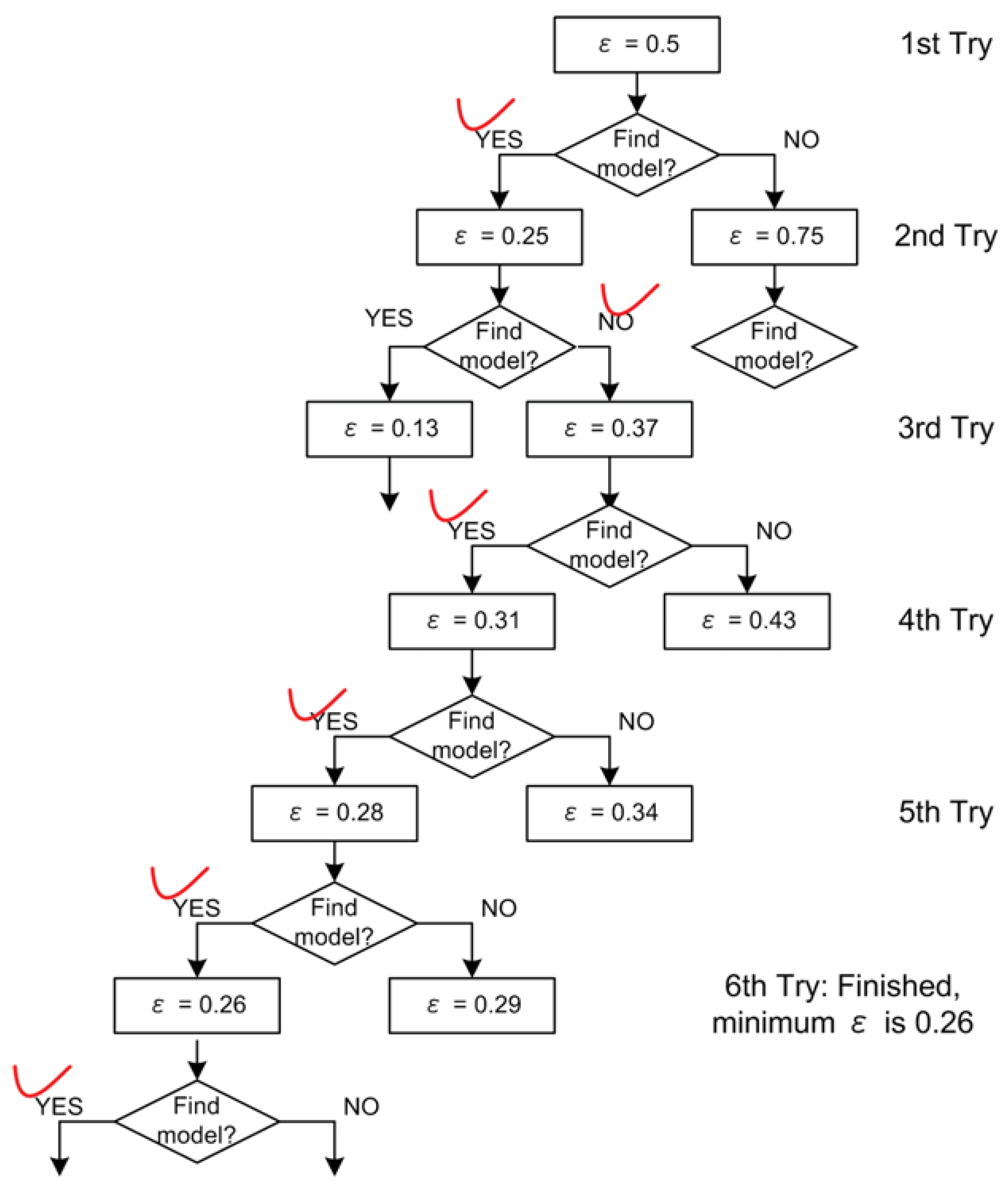
In the second method, the ϵ m can also be found with a manual binary search method. Since ϵ [ 0 , 1 ) , ϵ is specified to 0.5 in the first try. If the DFL algorithm finds a model with ϵ value of 0.5, then ϵ is specified to 0.25 in the second try. Otherwise, if the DFL algorithm cannot find a model with a long time, like 10 minutes, then the DFL algorithm can be stopped and ϵ is specified to 0.75 in the second try. The selection process is carried out until the ϵ m value is found so that the DFL algorithm can find a model with it but cannot when ϵ = ϵ m 0 . 01 . This selection process is also efficient. Since ϵ [ 0 , 1 ) , only 5 to 6 tries are needed to find the ϵ m on the average.
As shown in Figure 7, we use the LED data set [15] with 10 percent noise to show the manual binary search procedure. There are 3000 samples in this data set, 2000 as training and 1000 as testing. This LED data set will also be used later in Section 8. For this example, in the first try, DFL algorithm finds a model for the training data set with ϵ of 0.5. Then, the DFL algorithm cannot find a model with the ϵ of 0.25 in the second try. Similarly, from the third to sixth tries, the DFL algorithm finds models with the specified ϵ values, 0.37, 0.31, 0.28 and 0.26. Since we have known in the second try that the DFL algorithm cannot find a model with ϵ of 0.25. Hence, 0.26 is the minimum ϵ value for this data set.
The restricted learning process can also be used to find optimal feature subset. To get optimal feature subset, we change the ϵ value from 0 to the upper limit of the searching scope, like 0.8, with a step of 0.01. For each ϵ value, we train a model with the DFL algorithm, then validate its performance with cross validation or the testing data sets. The optimal model is the one which produces the best prediction performance. As demonstrated in Figure 6 (a), the optimal ϵ value, ϵ o p . = 0 . 31 , is chosen from the training data set with a 10-fold cross validation. The features of the optimal model are thus chosen as the optimal feature subsets that can be used by other classification algorithms. Actually, the features chosen by the DFL algorithm in the LED+17 training data are the 7 true relevant features when ϵ o p . = 0 . 31 , as shown in Figure 6 (b). Furthermore, Figure 6 (a) and (b) also demonstrate that both the optimal performance and optimal feature subsets are stable in the training and independent testing samples.

6. Prediction Method

After the DFL algorithm obtains the classifiers as function tables of the pairs ( u , y ) , or called as rules, the most reasonable way to use such function tables is to check the input values u , and find the corresponding output values y. This is due to the fact that the DFL algorithm is based on Theorem 4. As demonstrated in Section 3.4, the learned model of the DFL algorithm is actually the generation function as a truth table or an estimation of it in the ϵ value method. Like the way in which people use truth tables, it is advisable to use a classification model as a truth table, or the estimation of it, with the 1-Nearest-Neighbor algorithm [48] based on the Hamming distance [49]. In the prediction process, if a new sample is of same distance to several rules, we choose the rule with the biggest count value, which is obtained in the learning process. Although there exists the probability that some instances of the EAs in the testing data set are not covered by the training data set, the 1NN algorithm still gives the most reasonable predictions for such samples.

7. Implementation Issues

7.1. The Computation of Mutual Information I ( X ; Y )

As introduced in Section 1, it is not straightforward to compute high-dimensional MI. We will show how we deal with the problem. We use Equation 2 to compute I ( X ; Y ) . The H ( Y ) does not change in the searching process of the DFL algorithm. To compute H ( X ) and H ( X , Y ) , we need to estimate the joint distribution of X and ( X , Y ) , which can be estimated from the input table T . The DFL algorithm will construct a matrix containing the values of X . Then, it scans the matrix and finds the frequencies of different instances of X , which are stored in a frequency table with a linked list. The size of the frequency table grows exponentially with the number of variables in X , but will not exceed N. Next, the DFL algorithm will obtain the estimation of H ( X ) with Equation 1. For each instance of X in T , we need to update its frequency in the frequency table, which takes O ( m i n ( | | X | | , N ) ) steps. The total complexity to compute H ( X ) is O ( N · m i n ( | | X | | , N ) ) . The computation of H ( X ; Y ) is similar to that of H ( X ) . Hence, if X only contains a few variables, it will need approximate O ( N ) steps to compute I ( X ; Y ) , since | | X | | is small. While | X | is large, the computation of I ( X ; Y ) tends to take O ( N 2 ) steps in the worst case.
However, the complexity for computing I ( X ; Y ) can be improved by storing the frequencies of different instances of X and { X , Y } in a hash table [43]. For each instance of X in T , it only takes O ( 1 ) time to update its frequency in the hash table. Hence, the total complexity to compute H ( X ) is O ( N ) . The computation of H ( X ; Y ) is similar to that of H ( X ) . Therefore, it will only need approximate O ( N ) steps to compute I ( X ; Y ) . An important issue to note is the appropriate setting of the initial capacity of the hash table, since a too large value is a waste but too small value may incur the need to dynamically increase the capacity and to reorganize the hash table, which is time-consuming.
In summary, if | X | and N are large at the same time and there are enough memory space available, it is more advisable to use hash tables for calculating I ( X ; Y ) . While | X | or N is small and memory space is limited, it is better to use linked lists or arrays to compute I ( X ; Y ) .

7.2. Redundancy Matrix

The subroutine in Table 2 is recursive, which will introduce some redundant computation when the DFL algorithm exhaustively searches the searching space S K . As discussed in Section 3.5 and Figure 4, a feature subset with K features will be checked for K ! times in the worst case.
However, this redundant computation can be alleviated by storing the information that whether a subset has been checked or not with a Boolean type matrix. Let us consider the subsets with 2 variables. We introduce an n by n matrix called redundancy matrix, boolean R ( n × n ) . After a subset { X i , X j } and its supersets have been checked, R [ i ] [ j ] is assigned as true . Later, when the DFL algorithm is checking { X j , X i } , it will first check whether R [ i ] [ j ] or R [ j ] [ i ] is true. If yes, it will examine next subset. By doing so, the original worst time complexity becomes O ( ( n + 1 2 [ n 2 · 2 ! + + n K · K ! ] ) N + n K log n ) = O ( ( N + log n ) · n K ) . Although, this alleviated worst time complexity is in the same order as the original one, but it saves about half of the run time. The space complexity of R is O ( n 2 ) . But the type of R is boolean , so R will cost very limited memory space. In addition, if run time is more critical and the memory space is sufficient, higher dimensional matrices can be introduced to further reduce the run time of the DFL algorithm.
For instance, as shown in Figure 4, after introducing the redundancy matrix, the exhaustive searching of the DFL algorithm will take n + 1 / 2 * [ n 2 2 ! + n 3 3 ! + . . . + n K K ! ] = 34 steps, which is in the order of O ( n 4 ) = O ( 4 4 ) but much smaller than 4 4 . As shown in Figure 4 (b), there are totally 40 steps. But six of them marked as red regions, as well as their supersets, are not computed by checking the redundancy matrix.
To clearly show the implementation of the redundancy matrix R , an extended version of the main steps of the DFL algorithm is provided in supplementary materials. The usefulness of redundancy matrix is also validated in supplementary materials.

8. Results

8.1. Data Sets

We use the 24 data sets from the classic UCI machine learning repository [15] and high-dimensional gene (or protein) expression profiles in [16,17,18,19], as summarized in Table 5, to compare the DFL algorithm with other feature selection methods. We arrange the data sets in the ascending order of the number of features. In all the data sets used, the missing values are dealt as an independent state marked with “?".
For data sets with continuous features, we discretize their continuous features with the discretization algorithm introduced in [50]. The discretization is carried out in such a way that the training data set is first discretized. Then the testing data set is discretized according to the cutting points of variables determined in the training data set. For the Breast data set, the attributes are numerical with some limited integers. Therefore, we do not apply the pre-discretization method to this data set.
In this paper, we use the restricted learning method introduced in Section 5.2 to obtain optimal models for the DFL algorithm, with the searching scope of the ϵ from 0 to 0.8. As introduced in 5.1, K is set to n for data sets 1 to 14, and to 20 for other data sets. The detailed settings of the DFL algorithm and detailed results are given in supplementary materials.

8.2. Comparison with Other Feature Selection Methods

We implement the DFL algorithm with the Java language version 1.6. All experiments are performed on an HP AlphaServer SC computer, with one EV68 1 GHz CPU and 1 GB memory, running the Tru64 Unix operating system.
In this section, we compare the DFL algorithm with two well-known filter feature subset selection methods, the CFS method [20] and the CSE method [21], and the wrappers subset selection method, i.e., the WSE method [22]. The implementations of the CFS, CSE, and WSE algorithms in the Weka software [51] are used here because Weka is also developed with the Java language. As discussed in Section 2.1., the forward selection is used with the CFS, CSE and WSE feature subset selection methods.
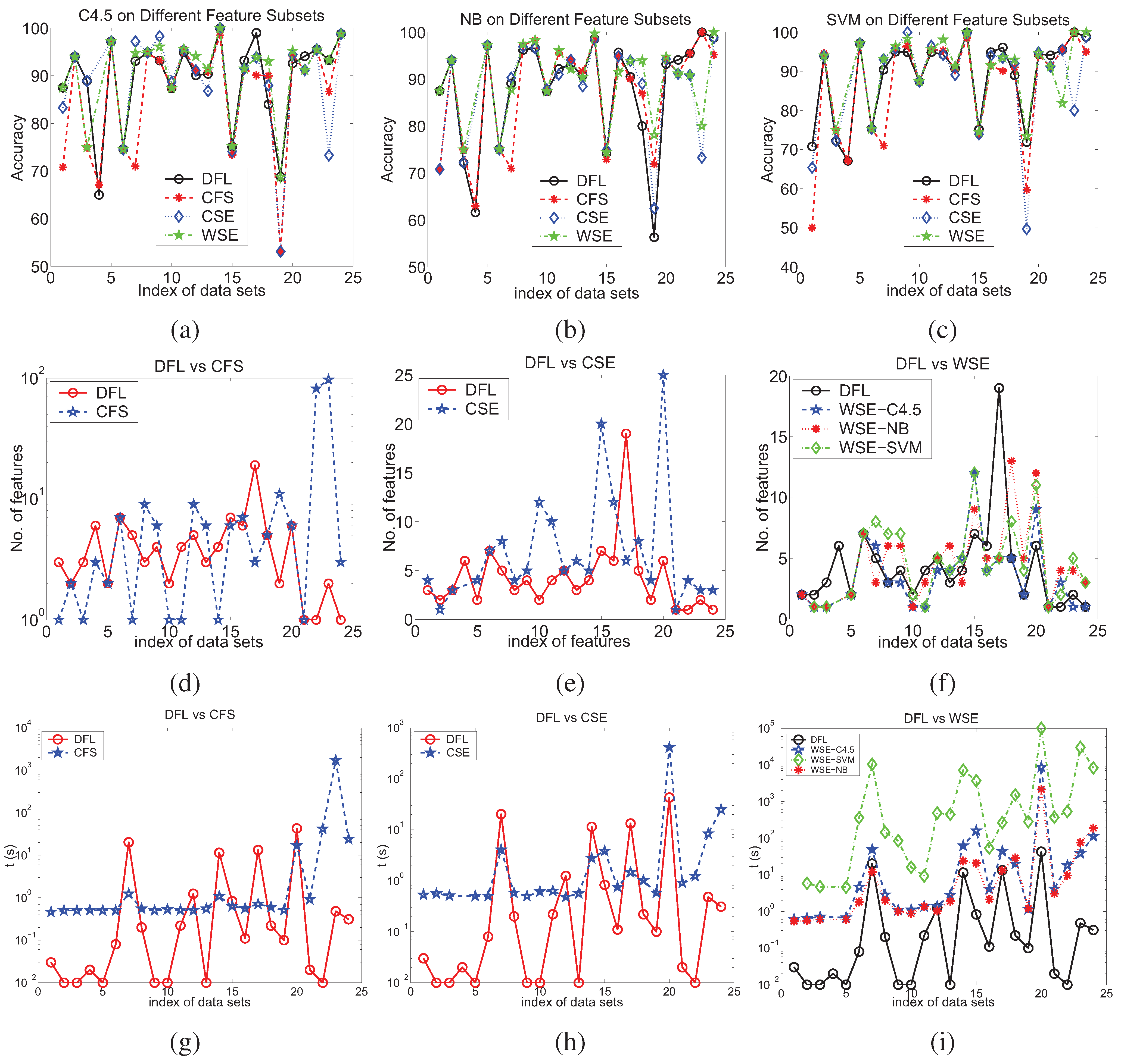
We choose three classification algorithms with different theoretical foundation, the C4.5 [52], Naive Bayes (NB) [53] and Support Vector Machines (SVM) algorithm [54] implemented by the Weka software, to validate different feature subset selection methods. For the SVM algorithm, the linear kernels are used. These algorithms are applied to the DFL, CFS, CSE, and WSE features with discretized values and original numerical values (see supplementary materials). The results for discretized values are shown in Figure 8. The results for original numerical values are shown in supplementary materials. Nevertheless, the results of both the discretized and numerical values are summarized in Table 7.
The CFS algorithm does not find a feature subset for the continuous MLL and Ovarian data sets. The CSE and WSE algorithm do not find a candidate feature subset for the Monk2 data set. In addition, the WSE algorithm when coupled with the SVM algorithm does not find a candidate feature subset for the Lenses data set. Therefore, the accuracies for these cases are not shown in Figure 8.
For four well-studies data sets, Monk1, Monk2, LED and LED+17, the DFL algorithm correctly and completely finds the true relevant features. From Figure 8, it is shown that the learning algorithms generally perform better on the DFL features when the number of features in the data sets is large, such as the data sets with index from 15 to 24, than on other features.
We also summarize the comparison of accuracies obtained by different feature selection methods in Table 7. For two feature selection methods, we count the number of data sets, where the classification algorithm applied to features of the first method performs better, equally to, or worse than applied to features of the second one.
From Table 7, it can be seen that the DFL algorithm generally chooses more discriminatory feature subsets than the CFS and CSE algorithm, as the learning algorithms show better prediction performances on the DFL features than on those chosen by the CFS and CSE algorithm, as in Table 7 row 4 and 8. The learning algorithms perform better, equally good and worse on the DFL features than on the WSE features in 16, 20 and 32 cases respectively, as in Table 7 last row.

8.3. Comparison of Model Complexity

The accuracy is only one aspect of the performances. The model complexity is another aspect of the performance of the feature selection algorithms. Thus, we also compare the number of features chosen by different feature selection methods, as shown in Figure 8d–8f.
We also summarize the number of features for different feature selection methods in Table 6. For two feature selection methods, we count the number of data sets, where the first method chooses smaller, equal, bigger number of features than the second one does. As summarized in Table 6, the DFL chooses comparable number of features to the CFS method, but less features than the CSE and WSE method.

8.4. Comparison of Efficiency

Next, we compare the run times of the DFL algorithm with other feature selection methods, as shown in Figure 8g–8i. In Figure 8g–8h, it is shown that the the DFL algorithm uses less time than the CFS and CSE algorithm in most data sets, 18 and 20 out of the 24 data sets respectively. The DFL algorithm is overwhelmingly faster than the WSE algorithm, Figure 8i. Especially for the high-dimensional data sets, those with index from 20 to 24, the DFL algorithm shows large reduction of run time when compared with other feature selection methods. These experimental results suggest that the DFL algorithm is faster than other feature selection methods that we have compared.

9. Discussions

The DFL algorithm can be categorized as a feature subset selection method or a filter method. However, the DFL algorithm is also different from other feature subset selection methods, like the CFS, CSE and WSE methods. Based on Theorem 4, the DFL algorithm can produce function tables for the training data sets, while other subset feature selection methods only generate a subset of features. Particularly, the DFL algorithm is different from existing feature subset selection methods based on information theory in the following three aspects.
First, the stopping criterion of the DFL algorithm is different from those of existing methods. The DFL algorithm stops the searching process based on Theorem 4. The existing methods stop the searching process with a predefined k or threshold value of MI. Hence, the feature subsets selected by existing methods may be sensitive to the k or threshold value of MI.
Second, the feature subset evaluation method of the DFL algorithm is different from those in existing methods [3,4,5,6,7,8,9,11,12,13]. The DFL algorithm uses Equation 14, i.e., X ( s ) = arg max i I ( U s 1 , X i ; Y ) , to evaluate a new feature. But existing methods evaluate a new feature with algebraic combinations of two dimensional MI, such as in Equations 5, 6, 7, 10, 11, 13 in Section 2.
Furthermore, the maximization of I ( U s 1 , X i ; Y ) used in the DFL algorithm is more efficient than penalizing the new feature with respect to every selected features, as done in [3,4,5,6,7,8,9,11,12,13]. As analyzed in Section 7.1., to evaluate I ( X ; Y ) , O ( n · N ) operations are needed when adding each feature, and O ( k · n · N ) operations are necessary to choose k features in the DFL algorithm. However, in calculating Equations 5, 6, 7, 10, 11, 13 in Section 2., since there are already ( s 1 ) features in U s 1 in the s iteration, there would be ( s 1 ) × O ( n · N ) operations in this iteration. Therefore, it needs s = 1 k ( s 1 ) × O ( n · N ) O ( k 2 · n · N ) operations to select k features, which is less efficient. The computational cost of the backward selection for approximating Markov Blanket is at least O ( 2 k · n · N ) [1], which is even worse than the O ( k 2 · n · N ) of the forward selection in [5,6]. In addition, the correlation matrix of all features needs to be computed in the approximation method of [1], which costs O ( n 2 ( log n + N ) ) operations.
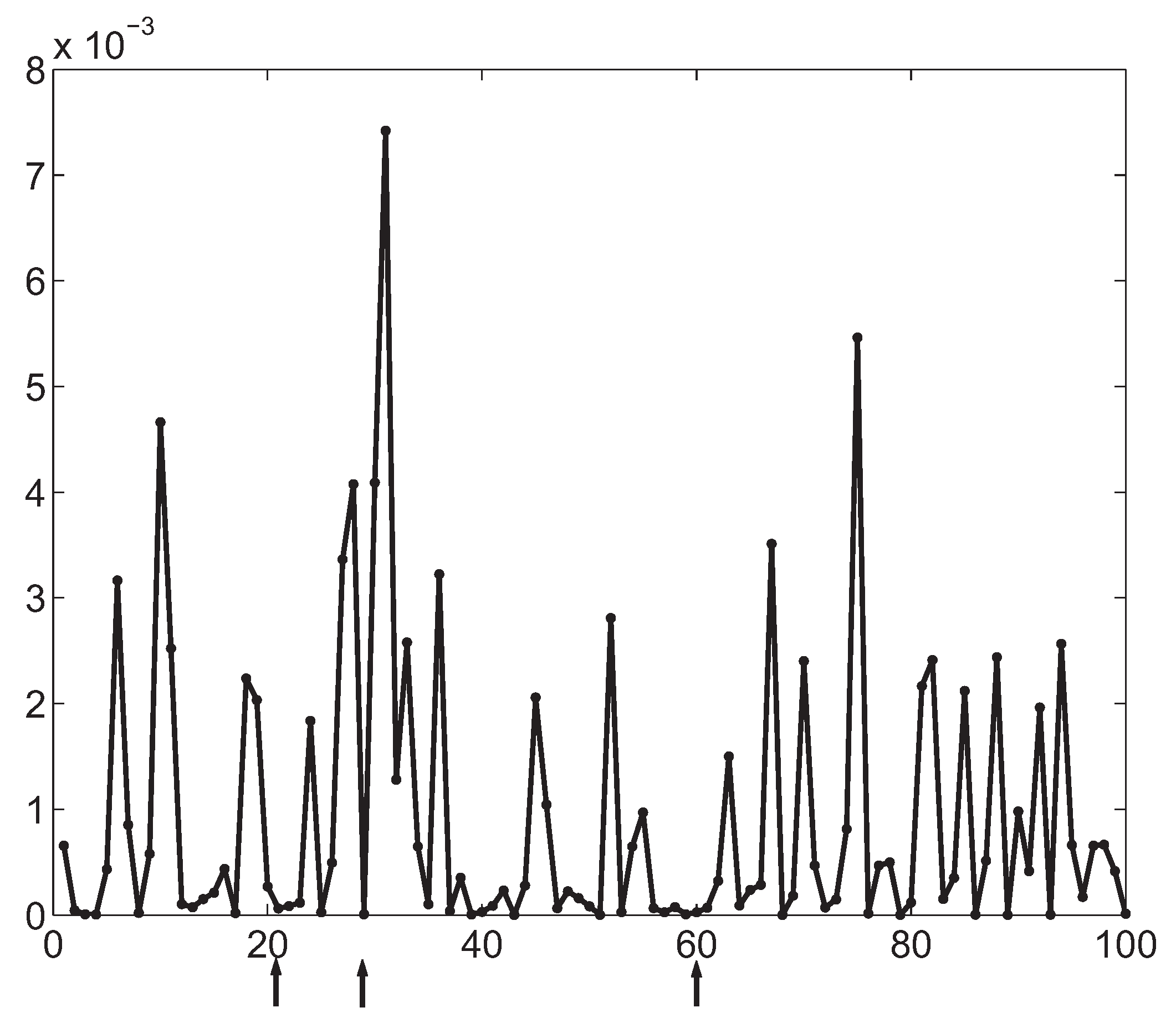
Third, the searching method used by the DFL algorithm is also different from the greedy (forward) selection searching [3,4,5,6,7,8,9,11,12,13] or the backward selection searching [1]. In the DFL algorithm, the exhaustive search of all subsets with K features is guaranteed and can be terminated with the criterion of Theorem 4. In some data sets, I ( X i ; Y ) = 0 , X i X , as demonstrated by the example in Figure 9. Existing feature selection methods based on MI [3,4,5,6,7,8,9,11,12,13] will fail for this kind of data sets. For the example in Figure 9, it is shown that the three true relevant features, X 21 , X 29 and X 60 , share smaller MI with Y than many other irrelevant features. Actually, based on Theorem 1, X i V , I ( X i ; Y ) should be zero in this data set since X i and Y are independent. But they are still larger than zero, although very small as shown in Figure 9, in practice. Hence, if a simple forward selection is used, existing feature selection methods will choose X 31 , which is an irrelevant feature, in the first round of the forward selection. Consider the selection criteria in Equation 5 [5,6] and Equation 10 [7]. First, I ( X i ; X j ) = 0 , since X i , X j V , X i and X j are independent. Second, X i V , X i and Y are independent. Consequently, the criteria in Equation 5 and Equation 10 will become X ( s ) = a r g m a x X i P I ( X i ; Y ) . In later rounds, many other irrelevant features will be added to the candidate feature subset, which will also be incorrect, since they have larger MI than the relevant features do. However, the DFL algorithm can still find the correct feature subsets in polynomial time for this kind of data sets, since it guarantees the exhaustive searching of all subsets with K features and evaluates all selected features as a vector with Equation 14. For the example in Figure 9, the DFL algorithm successfully finds the correct feature subsets with less than 15 minutes in each fold of a 10 fold cross validation and obtains 100% prediction accuracy in the cross validation in our experiment.
In summary, three unique properties of the DFL algorithm are prerequisite to solve feature selection problems introduced by the data sets with I ( X i ; Y ) = 0 , such as that in Figure 9. First, the candidate features are considered as a vector to compute I ( U ; Y ) . Second, I ( U ; Y ) is evaluated with respect to H ( Y ) based on Theorem 4, which guarantees to find the correct feature subset. Last, the searching schema of the DFL algorithm guarantees to exhaustively search all subsets of V with K features, although its first round searching is greedy forward selection.

10. Conclusion

It is critical to find optimal feature subsets to overcome the curse of dimensionality. As an endeavor to reach this goal, we prove that if I ( X ; Y ) = H ( Y ) , then X is a Markov Blanket of Y. We show that by comparing I ( U ; Y ) with H ( Y ) , the DFL algorithm can find the optimal and complete feature subsets in some cases. As shown in Section 8, the DFL algorithm successfully and completely finds the original relevant features for Monk1, Monk2, LED and LED+17 data sets without any prior knowledge.
We have proved the correctness of the DFL algorithm, discussed the implementation issues and its difference from existing methods. The usefulness of the DFL algorithm is validated with 24 benchmark data sets.
We also show that high dimensional MI is not equal to the algebraic combinations of pairwise ones. This conclusion is important and contributive since it can help to avoid other endeavors to find low-dimensional replacement of high-dimensional MI. We show that if for any individual relevant features X i , I ( X i ; Y ) = 0 , then (1) evaluating I ( U ; Y ) with Equation 14, instead of Equations 5, 6, 7, 10, 11, 13 in Section 2; (2) comparing I ( U ; Y ) with H ( Y ) ; and (3) the exhaustive search method are necessary to find correct feature subset.

Acknowledgements

The research was supported in part by a start-up grant of Fudan University and a grant of STCSM (10ZR1403000) to ZY and Singapore MOE AcRF Grant No: MOE2008-T2-1-1074 to KCK.

References and Notes

  1. Koller, D.; Sahami, M. Toward Optimal Feature Selection. In Proceedings of the 13th International Conference on Machine Learning, Bari, Italy, 3-6 July 1996; pp. 284–292.
  2. Hall, M.; Holmes, G. Benchmarking Attribute Selection Techniques for Discrete Class Data Mining. IEEE Trans. Knowl. Data Eng. 2003, 15, 1–16. [Google Scholar] [CrossRef]
  3. Battiti, R. Using mutual information for selecting features in supervised neural net learning. IEEE Trans. Neural Networks 1994, 5, 537–550. [Google Scholar] [CrossRef] [PubMed]
  4. Kwak, N.; Choi, C.H. Input feature selection for classification problems. IEEE Trans. Neural Networks 2002, 13, 143–159. [Google Scholar] [CrossRef] [PubMed]
  5. Vidal-Naquet, M.; Ullman, S. Object Recognition with Informative Features and Linear Classification; IEEE Computer Society: Nice, France, 2003; pp. 281–288. [Google Scholar]
  6. Fleuret, F. Fast Binary Feature Selection with Conditional Mutual Information. J. Mach. Learn. Res. 2004, 5, 1531–1555. [Google Scholar]
  7. Peng, H.; Long, F.; Ding, C. Feature Selection Based on Mutual Information: Criteria of Max-Dependency, Max-Relevance, and Min-Redundancy. IEEE Trans. Pattern Anal. Mach. Intell. 2005, 27, 1226–1238. [Google Scholar] [CrossRef] [PubMed]
  8. Bonev, B.; Escolano, F.; Cazorla, M. Feature selection, mutual information, and the classification of high-dimensional patterns. Pattern Anal. Appl. 2008, 11, 309–319. [Google Scholar] [CrossRef]
  9. Cai, R.; Hao, Z.; Yang, X.; Wen, W. An efficient gene selection algorithm based on mutual information. Neurocomputing 2009, 72, 991–999. [Google Scholar] [CrossRef]
  10. Zhu, S.; Wang, D.; Yu, K.; Li, T.; Gong, Y. Feature Selection for Gene Expression Using Model-Based Entropy. IEEE/ACM Trans. Comput. Biol. Bioinformatics 2010, 7, 25–36. [Google Scholar]
  11. Estévez, P.A.; Tesmer, M.; Perez, C.A.; Zurada, J.M. Normalized mutual information feature selection. Trans. Neur. Netw. 2009, 20, 189–201. [Google Scholar] [CrossRef] [PubMed]
  12. Martínez Sotoca, J.; Pla, F. Supervised feature selection by clustering using conditional mutual information-based distances. Pattern Recogn. 2010, 43, 2068–2081. [Google Scholar] [CrossRef]
  13. Vinh, L.T.; Thang, N.D.; Lee, Y.K. An Improved Maximum Relevance and Minimum Redundancy Feature Selection Algorithm Based on Normalized Mutual Information. IEEE/IPSJ Int. Symp. Appl. Internet 2010, 0, 395–398. [Google Scholar]
  14. Zheng, Y.; Kwoh, C.K. Identifying Simple Discriminatory Gene Vectors with An Information Theory Approach. In Proceedings of the 4th Computational Systems Bioinformatics Conference, CSB 2005, Stanford, CA, USA, 8-11 August 2005; pp. 12–23.
  15. Blake, C.; Merz, C. UCI Repository of Machine Learning Databases; UCI: Irvine, CA, USA, 1998. [Google Scholar]
  16. Golub, T.; Slonim, D.; Tamayo, P.; Huard, C.; Gaasenbeek, M.; Mesirov, J.; Coller, H.; Loh, M.; Downing, J.; Caligiuri, M.; Bloomfield, C.; Lander, E. Molecular Classification of Cancer: Class Discovery and Class Prediction by Gene Expression Monitoring. Science 1999, 286, 531–537. [Google Scholar] [CrossRef] [PubMed]
  17. Shipp, M.; Ross, K.; Tamayo, P.; Weng, A.; Kutok, J.; Aguiar, R.; Gaasenbeek, M.; Angelo, M.; Reich, M.; Pinkus, G.; Ray, T.; Koval, M.; Last, K.; Norton, A.; Lister, T.; Mesirov, J.; Neuberg, D.; Lander, E.; Aster, J.; Golub, T. Diffuse large B-cell lymphoma outcome prediction by gene-expression profiling and supervised machine learning. Nat. Med. 2002, 8, 68–74. [Google Scholar] [CrossRef] [PubMed]
  18. Armstrong, S.; Staunton, J.; Silverman, L.; Pieters, R.; den Boer, M.; Minden, M.; Sallan, S.; Lander, E.; Golub, T.; Korsmeyer, S. MLL translocations specify a distinct gene expression profile that distinguishes a unique leukemia. Nat. Genet. 2002, 30, 41–47. [Google Scholar] [CrossRef] [PubMed]
  19. Petricoin, E.; Ardekani, A.; Hitt, B.; Levine, P.; Fusaro, V.; Steinberg, S.; Mills, G.; Simone, C.; Fishman, D.; Kohn, E.; Liotta, L. Use of proteomic patterns in serum to identify ovarian cancer. Lancet 2002, 359, 572–577. [Google Scholar] [CrossRef]
  20. Hall, M. Correlation-based Feature Selection for Machine Learning. PhD thesis, Waikato University, Department of Computer Science, Hamilton, NewZealand, April 1999. [Google Scholar]
  21. Liu, H.; Setiono, R. A Probabilistic Approach to Feature Selection - A Filter Solution. In Proceedings of the 13th International Conference on Machine Learning, Bari, Italy, 3-6 July 1996; pp. 319–327.
  22. Kohavi, R.; John, G. Wrappers for Feature Subset Selection. Artif. Intell. 1997, 97, 273–324. [Google Scholar] [CrossRef]
  23. Liu, H.; Li, J.; Wong, L. A Comparative Study on Feature Selection and Classification Methods Using Gene Expression Profiles and Proteomic Patterns. Genome Inf. 2002, 13, 51–60. [Google Scholar]
  24. Xing, E.; Jordan, M.; Karp, R. Feature Selection for High-Dimensional Genomic Microarray Data. In Proceedings of the 18th International Conference on Machine Learning; Morgan Kaufmann Publishers Inc.: Williamstown, MA, USA 28 June–1 July 2001. ; pp. 601–608.
  25. Furey, T.; Cristianini, N.; Duffy, N.; Bednarski, D.; Schummer, M.; Haussler, D. Support vector machine classification and validation of cancer tissue samples using microarray expression data. Bioinformatics 2000, 16, 906–914. [Google Scholar] [CrossRef] [PubMed]
  26. van ’t Veer, L.; Dai, H.; van de Vijver, M.; He, Y.; Hart, A.; Mao, M.; Peterse, H.; van der Kooy, K.; Marton, M.; Witteveen, A.; Schreiber, G.; Kerkhoven, R.; Roberts, C.; Linsley, P.; Bernards, R.; Friend, S. Gene expression profiling predicts clinical outcome of breast cancer. Nature 2002, 415, 530–536. [Google Scholar] [CrossRef] [PubMed]
  27. Li, J.; Liu, H.; Downing, J.; Yeoh, A.; Wong, L. Simple rules underlying gene expression profiles of more than six subtypes of acute lymphoblastic leukemia (ALL) patients. Bioinformatics 2003, 19, 71–78. [Google Scholar] [CrossRef] [PubMed]
  28. John, G.; Kohavi, R.; Pfleger, K. Irrelevant Features and the Subset Selection Problem. In Proceedings of the 11th International Conference on Machine Learning, New Brunswick, NJ, USA, 10–13 July 1994; pp. 121–129.
  29. Shannon, C.; Weaver, W. The Mathematical Theory of Communication; University of Illinois Press: Urbana, IL, USA, 1963. [Google Scholar]
  30. Cover, T.M.; Thomas, J.A. Elements of Information Theory; John Wiley & Sons, Inc.: New York, NY, USA, 1991. [Google Scholar]
  31. Dumais, S.; Platt, J.; Hecherman, D.; Sahami, M. Inductive Learning Algorithms and Representations for Text Categorization. In Proceedings of the 7th International Conference on Information and Knowledge Management, Washington, DC, USA, 02-07 November 1998; pp. 148–155.
  32. Yang, Y.; Pedersen, J. A Comparative Study on Feature Selection in Text Categorization; Fisher, D.H., Ed.; Morgan Kaufmann Publishers: San Francisco, CA, US, 1997; pp. 412–420. [Google Scholar]
  33. Chow, T.W.S.; Huang, D. Estimating Optimal Features Subsets Using Efficient Estimation of High-Dimensional Mutual Information. IEEE Trans. Neural Networks 2005, 16, 213–224. [Google Scholar] [CrossRef] [PubMed]
  34. Maji, P. Mutual Information Based Supervised Attribute Clustering for Microarray Sample Classification. IEEE Trans. Knowl. Data Eng. 2010, 99. [Google Scholar]
  35. McEliece, R.J. Encyclopedia of Mathematics and Its Applications. In The Theory of Information and Coding: A Mathematical Framework for Communication; Addison-Wesley Publishing Company: Reading, MA, USA, 1977; Volume 3. [Google Scholar]
  36. Pearl, J. Probabilistic Reasoning in Intelligent Systems: Networks of Plausible Inference; Morgan Kaufmann: San Mateo, CA, USA, 1988. [Google Scholar]
  37. In [36], `-’ is used to denote the set minus(difference) operation. To be consistent to other parts of this paper, we will use `∖’ to denote the set minus operation. Particularly, AB is defined by AB = {X:XA and XB}.
  38. Yaramakala, S.; Margaritis, D. Speculative Markov Blanket Discovery for Optimal Feature Selection; IEEE Computer Society: Washington, DC, USA, 2005; pp. 809–812. [Google Scholar]
  39. Tsamardinos, I.; Aliferis, C. Towards Principled Feature Selection: Relevancy, Filters and Wrappers. In Proceedings of the Ninth International Workshop on Artificial Intelligence and Statistics; Bishop, C.M., Frey, B.J., Eds.; Morgan Kaufmann Publishers: Key West, FL, USA, 2003. [Google Scholar]
  40. Gray, R.M. Entropy and Information Theory; Springer Verlog: New York, NY, USA, 1991. [Google Scholar]
  41. Tsamardinos, I.; Aliferis, C.F.; Statnikov, A. Time and sample efficient discovery of Markov blankets and direct causal relations; ACM Press: New York, NY, USA, 2003; pp. 673–678. [Google Scholar]
  42. Aliferis, C.F.; Tsamardinos, I.; Statnikov, A. HITON: A novel Markov Blanket algorithm for optimal variable selection. AMIA Annu. Symp. Proc. 2003, 2003, 21–25. [Google Scholar]
  43. Cormen, T.; Leiserson, C.; Rivest, R.; Stein, C. Introduction to Algorithms, Second Edition; MIT Press: Cambridge, MA, USA, 2001. [Google Scholar]
  44. Except Δ1 supersets, only a part of other Δi(i = 2, ,K-1) supersets is stored in ΔTree.
  45. Akutsu, T.; Miyano, S.; Kuhara, S. Identification of genetic networks from a small number of gene expression patterns under the Boolean network model. In Proceedings of Pacific Symposium on Biocomputing ’99, Big Island, HI, USA, 4-9 January 1999; Volume 4, pp. 17–28.
  46. Zheng, Y.; Kwoh, C.K. Dynamic Algorithm for Inferring Qualitative Models of Gene Regulatory Networks; IEEE Computer Society Press: Stanford, CA, USA, 2004; pp. 353–362. [Google Scholar]
  47. Zheng, Y.; Kwoh, C.K. Dynamic Algorithm for Inferring Qualitative Models of Gene Regulatory Networks. Int. J. Data Min. Bioinf. 2006, 1, 111–137. [Google Scholar] [CrossRef]
  48. Aha, D.W.; Kibler, D.; Albert, M.K. Instance-Based Learning Algorithms. Mach. Learn. 1991, 6, 37–66. [Google Scholar] [CrossRef]
  49. Hamming, R. Error Detecting and Error Correcting Codes. Bell Syst. Techn. J. 1950, 9, 147–160. [Google Scholar] [CrossRef]
  50. Fayyad, U.; Irani, K. Multi-Interval Discretization of Continuous-Valued Attributes for Classification Learning. In Proceedings of the 13th International Joint Conference on Artificial Intelligence, IJCAI-93, Chambery, France, 28 August 1993; pp. 1022–1027.
  51. Frank, E.; Hall, M.; Trigg, L.; Holmes, G.; Witten, I. Data mining in bioinformatics using Weka. Bioinformatics 2004, 20, 2479–2481. [Google Scholar] [CrossRef] [PubMed]
  52. Quinlan, J. C4.5: Programs for Machine Learning; Morgan Kaufmann: San Francisco, CA, USA, 1993. [Google Scholar]
  53. Langley, P.; Iba, W.; Thompson, K. An Analysis of Bayesian Classifiers. In Proceedings of National Conference on Artificial Intelligence, San Jose, California, 12-16 July 1992; pp. 223–228.
  54. Platt, J. Fast training of support vector machines using sequential minimal optimization; MIT Press: Cambridge, MA, USA, 1999; Chapter 12; pp. 185–208. [Google Scholar]
  55. Zheng, Y. Information Learning Approach. PhD thesis, Nanyang Technological University, Singapore, 2007. [Google Scholar]
  56. Akutsu, T.; Miyano, S.; Kuhara, S. Algorithm for Identifying Boolean Networks and Related Biological Networks Based on Matrix Multiplication and Fingerprint Function. J. Computat. Biol. 2000, 7, 331–343. [Google Scholar] [CrossRef] [PubMed]
  57. Akutsu, T.; Miyano, S.; Kuhara, S. Inferring qualitative relations in genetic networks and metabolic pathways. Bioinformatics 2000, 16, 727–734. [Google Scholar] [CrossRef] [PubMed]
  58. Akutsu, T.; Miyano, S.; Kuhara, S. A simple greedy algorithm for finding functional relations: efficient implementation and average case analysis. Theor. Comput. Sci. 2003, 292, 481–495. [Google Scholar] [CrossRef]
  59. Ideker, T.; Thorsson, V.; Karp, R. Discovery of Regulatory Interactions Through Perturbation: Inference and Experimental Design. In Proceedings of Pacific Symposium on Biocomputing, PSB 2000, Island of Oahu, HI, January 4-9, 2000; 5, pp. 302–313.
  60. Lähdesmäki, H.; Shmulevich, I.; Yli-Harja, O. On Learning Gene Regulatory Networks Under the Boolean Network Model. Mach. Learn. 2003, 52, 147–167. [Google Scholar] [CrossRef]
  61. Liang, S.; Fuhrman, S.; Somogyi, R. REVEAL, a general reverse engineering algorithms for genetic network architectures. In Proceedings of Pacific Symposium on Biocomputing ’98, Maui, HI, USA, 4-9 January 1998; Volume 3, pp. 18–29.
  62. Maki, Y.; Tominaga, D.; Okamoto, M.; Watanabe, S.; Eguchi, Y. Development of a System for the Inference of Large Scale Genetic Networks. In Proceedings of Pacific Symposium on Biocomputing, PSB 2001, Big Island, HI, USA, 3-7 January 2001; 6, pp. 446–458.
  63. Schmulevich, I.; Yli-Harja, O.; Astola, J. Inference of genetic regulatory networks under the best-fit extension paradigm. In Presented at Nonlinear Signal and Image Processing, NSIP 2001, Baltimore, MD, USA, 3-6 June 2001; pp. 3–6.
Figure 1. The advantage of using MI to choose the most discriminatory feature vectors. The circles represent the entropy of variables or vectors. The intersection between the circles represents the MI between the variables or vectors. U s 1 is the features already chosen. The shaded regions represent I ( X i ; Y | U s 1 ) , where X i V U s 1 . (a) When X i = A . A shares less MI with Y than B does. However, the vector { U s 1 , A } shares larger MI with Y than the vector { U s 1 , B } does. (b) When X i = B . B shares larger MI with Y than A does. But B and U s 1 have a large MI, which means that U s 1 has contained most of the information of Y carried by B or the additional information of Y carried by B, I ( B ; Y | U s 1 ) , is small.
Entropy 13 00860 g001
Figure 2. The search procedures of the DFL algorithm when it is learning Y = ( A · C ) + ( A · D ) . { A , C , D } * is the target combination. The combinations with a black dot under them are the subsets which share the largest MI with Y on their layers. Firstly, the DFL algorithm searches the first layer, then finds that { A } , with a black dot under it, shares the largest MI with Y among subsets on the first layer. Then, it continues to search Δ 1 ( A ) on the second layer. Similarly, these calculations continue until the target combination { A , C , D } is found on the third layer.
Entropy 13 00860 g002
Figure 3. The Δ T r e e when searching the EAs for Y = ( A · C ) + ( A · D ) . (a) after searching the first layer of Figure 2 but before the sort step in line 7 of Table 2. (b) when searching the second layer of Figure 2. The { A } , { C } and { D } which are included in the EAs of Y are listed before { B } after the sort step in line 7 of Table 2. (c) when searching the third layer of Figure 2, { A , C , D } * is the target combination. Similar to part (b), the { A , C } and { A , D } are listed before { A , B } . When checking the combination { A , C , D } , the DFL algorithm finds that { A , C , D } is the complete EAs for Y since { A , C , D } satisfies the criterion of Theorem 4.
Entropy 13 00860 g003
Figure 4. The exhaustive searching procedures of the DFL algorithm when it is learning Y = ( A · C ) + ( A · D ) . { A , C , D } * is the target combination. (a) The exhaustive searching after the first round searching. The numbers beside the subsets are the steps of the DFL algorithm in part (b). The solid edges represent the searching path in the first round searching, marked as blue region in part (b). The dashed edges represent the searching path beyond the first round searching (only partly shown for the sake of legibility), marked as yellow regions in the table below. (b) The exhaustive searching steps. Blue, yellow and red regions correspond to first round searching, exhaustive searching and the subsets, as well as their supersets, not checked after deploying the redundancy matrix to be introduced in Section B.1.
Entropy 13 00860 g004
Figure 5. The Venn diagram of H ( X ) , H ( Y ) and I ( X , Y ) , when Y = f ( X ) . (a) The noiseless case, where the MI between X and Y is the entropy of Y. (b) The noisy case, where the entropy of Y is not equal to the MI between X and Y strictly. The shaded region is resulted from the noises. The ϵ value method means that if the area of the shaded region is smaller than or equal to ϵ × H ( Y ) , then the DFL algorithm will stop the searching process, and build the function for Y with X .
Entropy 13 00860 g005
Figure 6. The performance of the DFL algorithm for different ϵ values. The figures are generated from LED+17 data sets in Table 5. The training data set has 2000 samples and K is set to 20. The curves marked with circles and triangles are for result of 10-fold cross validation and the result of an independent testing data set of 1000 samples. The ϵ o p . pointed by an arrow is the optimal ϵ value with which the DFL algorithm reaches its highest prediction accuracy in a 10-fold cross validation for the training data set. (a) ϵ vs accuracy. (b) ϵ vs the number of selected features k. (c) ϵ vs the run time (s).
Entropy 13 00860 g006
Figure 7. The manual binary search of minimum ϵ value. This figure is generated with the LED training data set in Table 5, with 2000 samples. The ticks indicate whether the DFL algorithm can find a model after a ϵ value is specified in each try.
Entropy 13 00860 g007
Figure 8. The comparison of accuracies (a) to (c), number of features (d)-(f) and run time (g)-(i) for different feature subset selection methods on the discretized data sets. (a) C4.5, (b) NB, (c) SVM, (d) DFL vs CFS, (e) DFL vs CSE, (f) DFL vs WSE, (g) DFL vs CFS, (h) DFL vs CSE, (i) DFL vs WSE.
Entropy 13 00860 g008
Figure 9. The I ( X i ; Y ) in the data sets of 1000 samples generated with Y = ( X 21 X 29 X 60 ) , and V = { X 1 , , X 100 } , X i , X j V , X i and X j are independent. The horizontal axis is the index of the features. The vertical axis is the I ( X i ; Y ) shown in bits. The features pointed by the arrows are the relevant features.
Entropy 13 00860 g009
Figure 10. The histograms of the number of subsets checked, m, and run time of the DFL algorithm for learning one Boolean function in RANDOM data sets, when n = 100 , k = 3 and N = 200 . For part (b) and (c), the cases pointed by arrows are the worst ones. (a) The histogram of m without using redundancy matrix R . (b) The histogram of run time, t (horizontal axis, shown in seconds). (c) The histogram of run time after using the redundancy matrix R introduced in Section B.1..
Entropy 13 00860 g010
Table 1. The DFL algorithm.
Algorithm: DFL( V , K , T )
Input: a list V with n variables, indegree K,
T = { ( v i , y i ) : i = 1 , , N } . T is global.
Output: f
Begin:
1 L all single element subsets of V ;
2 Δ T r e e . F i r s t N o d e L ;
3calculate H ( Y ) ;   //from T
4 D 1 ;   //initial depth
5 * f = S u b ( Y , Δ T r e e , H ( Y ) , D , K ) ;
6return f;
End
* Sub() is a subroutine listed in Table 2.
Table 2. The subroutine of the DFL algorithm.
Algorithm: S u b ( Y , Δ T r e e , H , D , K )
Input: variable Y, Δ T r e e , entropy H ( Y )
current depth D, maximum indegree K
Output: function table for Y, Y = f ( X )
Begin:
1 L Δ T r e e . D t h N o d e ;
2for every element X L {
3  calculate I ( X ; Y ) ; //from T
4  if( I ( X ; Y ) = = H ) { //from Theorem 4
5    extract Y = f ( X ) from T ;
6    return Y = f ( X ) ;
  }
}
7sort L according to I;
8for every element X L {
9  if( D < K ){
10     D D + 1 ;
11     Δ T r e e . D t h N o d e Δ 1 ( X ) ;
12    return S u b ( Y , Δ T r e e , H , D , K ) ;
  }
}
13return “Fail(Y)"; //fail to find function for Y
End
Table 3. The training data set T of the example to learn Y = ( A · C ) + ( A · D ) .
ABCDYABCDYABCDYABCDY
00000010001000011000
00010010101001111011
00100011001010111101
00110011101011111111
Table 4. The learned classifier f of the example to learn Y = ( A · C ) + ( A · D ) .
ACDYCountACDYCount
0000210002
0010210112
0100211012
0110211112
Table 5. The benchmark data sets used in the experiments for comparison.
DatasetFtr. # 1 Cl. #Tr. #Te. #Ms. #Reference
1Lenses4324LOO 2 0[15]
2Iris43100500[15]
3Monk1621244320[15]
4Monk2621694320[15]
5Monk3621224320[15]
6LED710200010000[15]
7Nursery8512960CV10 3 0[15]
8Breast92699CV1016[15]
9Wine133119590[15]
10Credit15246023067[15]
11Vote162435CV10392[15]
12Zoo167101LOO0[15]
13ImgSeg19721021000[15]
14Mushroom2228124CV102480[15]
15LED+172410200010000[15]
16Ionosphere3422341170[15]
17Chess362213010660[15]
18Anneal38679810022175[15]
19Lung56332LOO0[15]
20Ad15582218610932729[15]
21ALL7129238340[16]
22DLBCL7129255220[17]
23MLL12582357150[18]
24Ovarian151542169840[19]
Ftr. #, Cl. #, Tr. #, Te. #, Ms. # and Ref. stand for the numbers of features, classes, training samples, testing samples, missing values and reference respectively. 1 The number does not include the class attribute. 2 LOO and 3 CV10 stands for leave-one-out and 10 fold cross validation respectively.
Table 6. The comparison summary of the number of features chosen by different feature selection methods.
Discretized D. S.Continuous D. S.
F.S. PairAlgo. < 1 =><=>
DFL:CFSNA 2 968769
DFL:CSENA17421751
DFL:WSEC4.5698878
NB1049977
SVM12551354
sub sum281822302117
total sum542634543029
1 The <, = and > column stand for the number of data sets, where the DFL algorithm chooses smaller, the same and larger number of features than the compared feature selection algorithm. 2 NA means not applicable.
Table 7. The comparison summary of accuracies obtained by different feature selection methods.
Discretized D.S.Continuous D.S.
F.S. PairAlgo. > 1 =<>=<
DFL:CFSC4.511761354
NB868859
SVM1257967
sum311821301620
DFL:CSEC4.5878968
NB8691058
SVM11751058
sum272022291624
DFL:WSEC454109779
NB74127412
SVM56114513
sum162032181634
1 The >, = and < column stand for the number of data sets, where the classification algorithm in the Algo. column performs better, the same and worse on the features chosen by the DFL algorithm.
Table 8. The extended version of the DFL algorithm.
Algorithm: DFL( V , K , T )
Input: a list V with n variables, indegree K,
T = { ( v i , y i ) : i = 1 , , N } . T is global.
Output: f
Begin:
1 R boolean[n][n];   //initialize R , default value is false
2 L all single element subsets of V ;
3 Δ T r e e . F i r s t N o d e L ;
4calculate H ( Y ) ;   //from T
5 D 1 ;   //initial depth
6 * f = S u b ( Y , Δ T r e e , H ( Y ) , D , K ) ;
7return f;
End
* Sub() is a subroutine listed in Table 9.
Table 9. The extended version of the subroutine of the DFL algorithm.
Algorithm: S u b ( Y , Δ T r e e , H , D , K )
Input: variable Y, Δ T r e e , entropy H ( Y ) , current depth D, maximum indegree K
Output: function table for Y, Y = f ( X )
Begin:
1 L Δ T r e e . D t h N o d e ;
2for every element X L {
3 *   if ( ( | X | = = 2 ) && ( R [ X [ 0 ] ] [ X [ 1 ] ] = = true | | R [ X [ 1 ] ] [ X [ 0 ] ] = = true) ) {
4    continue;  //if X has been checked, continue to check next element in L
  }
5  calculate I ( X ; Y ) ; //from T
6  if( I ( X ; Y ) = = H ) { //from Theorem 4
7    extract Y = f ( X ) from T ;
8    return Y = f ( X ) ;
  }
9  else if ( D = = K ) && X is the last element in L) {
10    return “Fail(Y)";
  }
}
11sort L according to I;
12for every element X L {
13  if( D < K ){
14    if ( ( | X | = = 2 ) && ( R [ X [ 0 ] ] [ X [ 1 ] ] = = true | | R [ X [ 1 ] ] [ X [ 0 ] ] = = true) ) {
15      continue;
    }
16     D D + 1 ;
17     Δ T r e e . D t h N o d e Δ 1 ( X ) ;
18     f = S u b ( Y , Δ T r e e , H , D , K ) ;
19    if f “Fail(Y)" {
20      return f;
    }
21    else if ( | X | = = 2 ) {
22       R [ X [ 0 ] ] [ X [ 1 ] ] true ; //if all Δ ( X ) have been checked, set R [ · ] [ · ] to true.
23      continue;
    }
  }
}
24return “Fail(Y)"; //fail to find function for Y
End
* The && and || represent the logic AND and OR operations respectively.
Table 10. The settings of the DFL algorithm. To get optimal model, we change the epsilon value from 0 to 0.8, with a step of 0.01. For each epsilon value, we train a model with the DFL algorithm, then do corresponding test for the selected data sets. In our implementation of the DFL algorithm, the process to choose optimal model can be automatically fulfilled. For those data sets whose testing processes are performed with the cross validation, the number of features k and the number of the rules r in the classifier are from the most frequently obtained classifiers.
PerformancesSettingsClassifiers
Data SetAccuracy (%)Time(s)nKϵkr k / n (%)
1Lenses75.00.03440.2631275.0
2Iris96.00.01440.082650.0
3Monk1100.00.0166033550.0
4Monk273.80.02660.216168100.0
5Monk397.20.01660.6421733.3
6LED74.90.08770.297207100.0
7Nursery93.120.21880.13554162.5
8Breast95.00.20990.05318533.3
9Wine98.30.0113130.0442930.8
10Credit88.30.0115150.5721113.3
11Vote95.70.2216160.1144125.0
12Zoo92.81.241616052131.3
13ImgSeg90.60.0119150.1634115.8
14Mushroom100.011.452222049618.2
15LED+1775.40.8324200.31728629.2
16Ionosphere94.90.1134200.1269617.6
17Chess97.413.3036200.011984452.8
18Anneal99.00.2238200.0454413.2
19Lung62.50.1056200.442123.6
20Ad95.042.801558200.2361040.4
21ALL94.10.027129200.3130.014
22DLBCL95.50.017129200.52140.014
23MLL100.00.4812582200.062110.016
24Ovarian98.80.3115154200.29140.007
average91.03.821829140.20411731.5
Table 11. The features chosen by the DFL algorithm.
Feature Index
Data SetkDiscretized DataContinuous Data
1Lenses21,3,41,3,4
2Iris23,43,4
3Monk131,2,51,2,5
4Monk261,2,3,4,5,61,2,3,4,5,6
5Monk322,52,5
6LED71,2,3,4,5,6,71,2,3,4,5,6,7
7Nursery51,2,5,7,81,2,5,7,8
8Breast31,3,61,3,6
9Wine41,7,10,131,7,10,13
10Credit24,94,9
11Vote43,4,7,113,4,7,11
12Zoo53,4,6,9,133,4,6,9,13
13 * ImgSeg31,13,152,17,19
14Mushroom45,20,21,225,20,21,22
15LED+1771,2,3,4,5,6,71,2,3,4,5,6,7
16Ionosphere63,5,6,12,21,273,5,6,12,21,27
17Chess191,3,4,6,7,10,15,16,17,18,20,1,3,4,6,7,10,15,16,17,18,20,
21,23,24,30,32,33,34,3521,23,24,30,32,33,34,35
18Anneal53,5,8,9,123,5,8,9,12
19Lung26,206,20
20Ad61,2,3,352,1244,14001,2,3,352,1244,1400
21 * ALL12341882
22 * DLBCL155506
23 * MLL2709,15502592,5083
24 * Ovarian18391679
* For these 5 data sets, the discretized data sets is preprocessed by deleting the features with only 1 value. Hence, the index of discrete data sets are different from those for continuous data sets.
Table 12. The accuracies of different algorithms on the features chosen by the DFL algorithm. The accuracies for those data sets with numerical attributes are for discretized/numerial data sets.
Data SetC4.5NBSVM
1Lenses87.575.066.7
2Iris94.0/92.094.0/94.094.0/96.0
3Monk188.972.272.2
4Monk265.061.667.1
5Monk397.297.297.2
6LED74.675.175.3
7Nursery93.189.190.4
8Breast94.896.295.0
9Wine93.2/93.296.6/98.394.9/98.3
10Credit87.4/87.487.4/87.487.4/87.4
11Vote94.992.294.9
12Zoo90.193.194.3
13ImgSeg90.4/90.890.8/84.390.7/76.1
14Mushroom100.098.6100.0
15LED+1775.174.275.1
16Ionosphere93.2/94.995.7/94.094.9/80.3
17Chess99.090.596.1
18Anneal84.0/84.080.0/74.089.0/88.0
19Lung68.856.371.9
20Ad92.6/94.493.2/92.494.4/92.6
21ALL94.1/94.194.1/94.194.1/82.4
22DLBCL95.5/95.595.5/90.995.5/77.3
23MLL93.3/93.3100.0/100.0100.0/73.3
24Ovarian98.8/98.898.8/98.898.8/97.6
average89.4/89.587.4/86.788.7/85.2
Table 13. The accuracies of different algorithms on the features chosen by the CFS algorithm [20]. The accuracies for those data sets with numerical attributes are for discretized/numerial data sets. NA means not available.
Data SetC4.5NBSVM
1Lenses70.870.850.0
2Iris94.0/92.094.0/94.094.6/96.0
3Monk175.075.075.0
4Monk267.163.067.1
5Monk397.297.297.2
6LED74.675.175.3
7Nursery71.071.071.0
8Breast94.797.395.8
9Wine93.2/93.298.3/98.396.6/96.6
10Credit87.4/87.487.4/87.487.4/87.4
11Vote95.695.695.6
12Zoo91.194.195.3
13ImgSeg90.9/90.391.7/86.090.3/87.9
14Mushroom98.598.598.5
15LED+1773.472.973.8
16Ionosphere91.5/93.294.9/93.291.5/80.3
17Chess90.190.190.1
18Anneal90.0/92.087.0/64.091.0/81.0
19Lung53.171.959.7
20Ad94.2/94.194.4/93.294.1/92.9
21ALL91.2/91.291.2/91.291.2/79.4
22DLBCL95.5/86.495.5/95.595.5/81.8
23MLL86.7/NA100.0/NA100.0/NA
24Ovarian98.8/NA95.2/NA95.0/NA
average86.1/85.187.6/85.286.3/83.1
Table 14. The accuracies of different algorithms on the features chosen by the CSE algorithm [21]. The accuracies for those data sets with numerical attributes are for discretized/numerial data sets. NA means not available.
Data SetC4.5NBSVM
1Lenses83.370.865.4
2Iris94.0/92.094.0/94.094.0/92.0
3Monk188.972.272.2
4Monk2NANANA
5Monk397.297.297.2
6LED74.675.175.3
7Nursery97.290.393.1
8Breast94.996.995.8
9Wine98.3/96.696.6/94.1100.0/100.0
10Credit88.7/86.187.8/80.487.4/87.4
11Vote95.491.096.5
12Zoo91.194.194.2
13ImgSeg86.8/90.388.5/80.889.1/80.3
14Mushroom100.098.599.7
15LED+1774.174.973.9
16Ionosphere91.5/92.394.9/94.094.0/81.2
17Chess93.993.993.5
18Anneal88.0/89.089.0/64.092.0/83.0
19Lung53.162.549.7
20Ad94.4/94.694.2/93.794.8/93.7
21ALL91.2/91.291.2/91.291.2/79.4
22DLBCL95.5/95.590.9/86.495.5/77.3
23MLL73.3/66.773.3/66.780.0/46.7
24Ovarian98.8/100.098.8/100.098.8/100.0
average88.9/88.687.7/85.388.0/83.8
Table 15. The accuracies of different algorithms on the features chosen by the WSE algorithm [22]. The accuracies for those data sets with numerical attributes are for discretized/numerial data sets. NA means not available.
Data SetC4.5NBSVM
1Lenses87.587.5NA
2Iris94.0/92.094.0/94.094.0/96.0
3Monk175.075.075
4Monk2NANANA
5Monk397.297.297.2
6LED74.675.175.3
7Nursery94.887.893.1
8Breast95.097.596.4
9Wine96.1/93.298.3/96.698.3/94.9
10Credit87.4/86.187.4/87.487.4/87.4
11Vote95.696.195.6
12Zoo94.192.198.1
13ImgSeg91.4/91.590.4/87.291.4/87.8
14Mushroom100.099.7100.0
15LED+1775.274.474.5
16Ionosphere91.5/85.591.5/91.591.5/86.3
17Chess93.993.993.5
18Anneal93.0/95.094.0/90.093.0/92.0
19Lung68.878.173.4
20Ad95.2/95.294.8/94.294.7/95.0
21ALL91.2/91.291.2/91.291.2/73.5
22DLBCL95.5/90.990.9/81.881.8/86.4
23MLL93.3/73.380.0/80.0100.0/93.3
24Ovarian98.8/100.0100.0/100.0100.0/100.0
average90.4/88.989.9/89.190.7/89.3

Supplementary Materials

A. The Software

We have implemented the DFL algorithm with the Java language version 1.6 [14,55]. The non-commercial license of the implementation software, called Discrete Function Learner, is available upon request.
The experiments are conducted on an HP AlphaServer SC computer, with one EV68 1 GHz CPU and 1 GB memory, running Tru64 Unix operating system.

B. The Extended Main Steps of The DFL Algorithm

B.1. Redundancy Matrix

As discussed in the paper, a feature subset with K features will be checked for K ! times in the worst case.
However, this redundant computation can be relieved by storing whether a subset has been checked or not with a Boolean type matrix. Let us consider the subsets with 2 variables. We introduce an n by n matrix called redundancy matrix, boolean R ( n × n ) , after a subset { X i , X j } and its supersets have been checked, R [ i ] [ j ] is assigned as true . Later, when the DFL algorithm is trying { X j , X i } , it will first check whether R [ i ] [ j ] or R [ j ] [ i ] is true. If yes, it will examine next subset. By doing so, the original worst time complexity becomes O ( ( n + 1 2 [ n 2 · 2 ! + + n K · K ! ] ) N + n K log n ) = O ( ( N + log n ) · n K ) . Although, this alleviated worst time complexity is in the same order as the original one, but it saves about half of the run time. The space complexity of R is O ( n 2 ) . But the type of R is boolean , so R will cost very limited memory space. In addition, if run time is more critical and the memory space is sufficient, higher dimensional matrices can be introduced to further reduce the run time of the DFL algorithm.

B.2. Extended Main Steps

The extended main steps of the DFL algorithm are listed in Table 8. As shown in line 21 to 23 of Table 9, R [ X [ 0 ] ] [ X [ 1 ] ] will be set to true if all Δ supersets of X have been checked. When the DFL algorithm is trying to check X later, it will find that X and its Δ supersets have been checked in line 3 and 14 respectively. For instance, { A , B } has been checked when the DFL algorithm is examining the supersets of { A } . Later, when it trying supersets of { B } , the DFL algorithm will revisit { A , B } , but this time the computation of { A , B } and its supersets will be saved by checking R . Thus, the computation of all subsets with equal to or more than 2 elements is reduce to half of the original computation without introducing redundancy matrix R , as analyzed in Section B.1.

B.3. Experiments to Show The Usefulness of Redundancy Matrix

The complexity of the DFL algorithm has been validated with comprehensive experiments elsewhere [47,55]. Here, we will validate the usefulness of the redundancy matrix in reducing run times.
We first present the synthetic data sets of Boolean networks [45,47,56,57,58,59,60,61,62,63]. For a Boolean network consisting of n genes, the total state space would be 2 n . The v of a transition pair is randomly chosen from 2 n possible instances of V with the Discrete Uniform Distribution, i.e., p ( i ) = 1 2 n , where i is randomly chosen one value from 0 to 2 n 1 inclusively. Since the DFL algorithm examines different subsets in the kth layer of Δ T r e e with lexicographic order, the run time of the DFL algorithm may be affected by the different position of the target subsets in the kth layer of Δ T r e e . Therefore, we select the first and the last k variables in V as the inputs for all X i . The data sets generated from the first k and last k variables are named as “head" and “tail" data sets. There are 2 2 k different Boolean functions when the indegree is k. Then, we use OR function (OR), AND function (AND), or one of the Boolean functions randomly selected from 2 2 k possible functions (RANDOM) to generate the v , i.e., f 1 = f 2 = = f n . If a data set is generated by OR function defined with the first or last k variables, then we name it as an OR-h or OR-t (OR-tail) data set, and so on.
Next, we generate 200 data sets, 100 RANDOM-h and 100 RANDOM-t data sets, with Boolean functions of indegree k = 3 randomly chosen from 2 2 3 functions. The DFL algorithm counts the checked subsets for inferring one Boolean function, denoted with m. The histogram of m is shown in Figure 10 (a). The run times for these data sets are shown in Figure 10 (b).
From Figure 10 (a), it is shown that the original Boolean function for X i can be found after checking O ( k · n ) subsets in 178 of out the 200 random functions. The complexity of the DFL algorithm will become O ( k · ( N + log n ) · n 2 ) for reconstructing the Boolean networks for the 178 random functions. The corresponding run times of the 178 cases are only a few seconds, as demonstrated in Figure 10 (b). As shown in Figure 10 (a), for 20 out of the remaining 22 cases, the original Boolean function for X i can be found after checking several thousands or less than n 2 subsets of V . The last two cases are learned after the DFL algorithm checked less than n 3 = 10 6 subsets of V . The last two cases are generated with special Boolean functions, similar to X i = X 1 · ¬ X 2 · ¬ X 3 + ¬ X 1 · X 2 · X 3 . In these Boolean functions, I ( X i j ; X i ) is zero, which makes the DFL algorithm be more computationally complex than for other data sets. In summary, the worst time complexity of the DFL algorithm, O ( N · n k ) , happens with about 2 / 200 = 1 % frequency for inferring random Boolean functions with indegree of 3.
For the 200 RANDOM data sets, the DFL algorithm finds the correct Boolean networks in 196 cases, and finds 2/3 correct edges of the original Boolean networks in the remaining 4 cases. Hence, the average sensitivity of the DFL algorithm is 596 / 600 99 . 3 % for inferring general Boolean networks from noiseless data sets.
From the experimental results for general Boolean networks, it is known that the DFL algorithm can find most Boolean functions with k inputs in O ( k · ( N + log n ) · n ) time.
To prove the usefulness of the redundancy matrix R introduced in Section B.1., we also perform the same experiments on these 200 RANDOM data sets after deploying the redundancy matrix in the DFL algorithm. Figure 10 (c) demonstrates that the run time of the worst case has been reduced from 203 to 127 seconds, which equals to a reduction of 37%. This is slightly smaller than the 50% reduction analyzed in Section B.1. We attribute this to the access and exchange of the memory used by R .

C. The Detailed Settings

For data sets with continuous features, we discretize their continuous features with the discretization algorithm introduced in [50]. The discretization is carried out in such a way that the training data set is first discretized. Then the testing data set is discretized according to the cutting points of variables determined in the training data set. For the Breast data set, the attributes are numerical with some limited integers. Therefore, we do not apply the pre-discretization method to this data set.
In this paper, we use the restricted learning method introduced in the paper to obtain optimal models for the DFL algorithm, with the searching scope of the ϵ from 0 to 0.8. As introduced in paper, K is set to n for data sets 1 to 14, and to 20 for other data sets. We have implemented the DFL algorithm with the Java language version 1.4.1 [14,55]. The experiments are conducted on an HP AlphaServer SC computer, with one EV68 1GHz CPU and 1GB memory, running Tru64 Unix operating system.
Table 10 gives the settings of the DFL algorithm for the used data sets. The features chosen by the DFL algorithm for them are given in Table 11.

D. The Detailed Results

In this section, we compare the DFL algorithm with two well-known filter feature subset selection methods, the CFS method by Hall [20] and the CSE method by Liu and Setiono [21], and the wrappers subset selection method, i.e., the WSE method, by Kohavi and John [22]. We use the CFS, CSE and WSE implemented by the Weka software [51] to compare their results with those from the DFL algorithm. The forward selection is used with the CFS, CSE and WSE feature subset selection methods.
We choose three classification algorithms with different theoretical foundation, the C4.5 [52], Naive Bayes (NB) [53] and Support Vector Machines (SVM) algorithm [54] implemented in the Weka software, to validate different feature subsets selection methods. For the SVM algorithm, the linear kernels are used. These algorithms are applied to the DFL, CFS, CSE, and WSE features with discretized values and original numerical values.
The DFL algorithm is used to choose feature for discretized data sets. Then, discretized and continuous values for the features chosen by the DFL algorithm are used to build classification models. The prediction accuracies of different classification algorithms on the DFL features are shown in Table 12. The CFS, CSE and WSE algorithm are applied to discretized and continuous data sets to choose features respectively. The prediction accuracies for the CFS, CSE and WSE features are shown in Table 13, Table 14 and Table 15 respectively.
The CFS algorithm does not find a feature subset for the continuous MLL and Ovarian data sets. The CSE and WSE algorithm do not find a candidate feature subset for the Monk2 data set. In addition, the WSE algorithm when coupled with the SVM algorithm does not find a candidate feature subset for the Lenses data set. Therefore, the accuracies for these cases are shown as NA (not available) in Table 13, Table 14 and Table 15.