A Survey on Interference Networks: Interference Alignment and Neutralization

Abstract

In recent years, there has been rapid progress on understanding Gaussian networks with multiple unicast connections, and new coding techniques have emerged. The essence of multi-source networks is how to efficiently manage interference that arises from the transmission of other sessions. Classically, interference is removed by orthogonalization (in time or frequency). This means that the rate per session drops inversely proportional to the number of sessions, suggesting that interference is a strong limiting factor in such networks. However, recently discovered interference management techniques have led to a paradigm shift that interference might not be quite as detrimental after all. The aim of this paper is to provide a review of these new coding techniques as they apply to the case of time-varying Gaussian networks with multiple unicast connections. Specifically, we review interference alignment and ergodic interference alignment for multi-source single-hop networks and interference neutralization and ergodic interference neutralization for multi-source multi-hop networks. We mainly focus on the “degrees of freedom” perspective and also discuss an approximate capacity characterization.

1. Introduction

Characterizing the capacity of Gaussian networks is a fundamental problem in network information theory. (Unless otherwise specified, we assume Gaussian networks having a single antenna at each node throughout the paper.) Unfortunately, even for the simplest setting of a single source and a single destination with a single relay, the capacity is not completely characterized for general channel parameters [1]. Recent applications of interest involve networks with multiple source–destination (SD) pairs (which we will also refer to as multiple “sessions”), and the capacity characterization appears to be much more challenging for these networks. One of the main difficulties for multi-source networks arises from the fact that the transmission of other sessions acts as interference and, as a result, how to efficiently manage interference from other sessions is of crucial importance for overall network performance. Exact capacity results being notoriously difficult to obtain, many researchers have recently studied approximate capacity characterizations in the shape of so-called “degrees of freedom” for multi-source networks. Degrees of freedom capture the behavior of capacity as the signal-to-noise ratio (SNR) becomes large, and they are believed to provide insight into the fundamental characteristics of multi-source networks. In recent years, there has been significant progress on this area and new coding paradigms have emerged. The aim of this paper is to review recent achievements relating to the capacity characterization of multi-source networks.

1.1. Traditional Approaches

For multi-source networks consisting of multiple SD pairs, the dominant feature is the interference between multiple sessions. In existing wireless communication systems, two approaches of dealing with interference are predominant. On the one hand, in some systems, interference is avoided by orthogonalization, meaning for example that at any given point in time (or frequency), only a single transmitter is active. On the other hand, interference is sometimes ignored and thus, treated as additional noise, meaning that communication strategies are employed that can deal with an increased noise level. These simple strategies have widely been adapted to cell planning in cellular systems and collision avoidance and detection protocols in media access control.

From a fundamental perspective, however, these two approaches are insufficient to attain optimal performance. It was proved in [2] that decoding interference first and then decoding the intended message can enlarge an achievable rate region of the 2-user interference channel depicted in Figure 1, compared with orthogonalization and treating interference as additional nose when the cross channel gains $|h_{21}{|}^2$ and $|h_{12}{|}^2$ are large enough. For example, destination 1 first decodes $W_2,$ then reconstructs the full signal transmitted by transmitter 2 and subtracts this interference signal from the received signal. Thus, destination 1 has removed all interference from the other transmitter and can now decode $W_1$. In the same manner, destination 2 first decodes $W_1$ and removes all interference. More generally, each message can be divided into common and private messages, i.e., $W_1=(W_1^{\mathsf{c}},W_1^{\mathsf{p}})$ and $W_2=(W_2^{\mathsf{c}},W_2^{\mathsf{p}})$, and each destination can decode a part of interfering message. That is, destination 1 decodes $(W_1^{\mathsf{c}},W_1^{\mathsf{p}},W_2^{\mathsf{c}})$ and destination 2 decodes $(W_2^{\mathsf{c}},W_2^{\mathsf{p}},W_1^{\mathsf{c}})$ [3]. Recently, this rate splitting with decoding a part of interfering message has been shown to achieve the capacity of the 2-user interference channel to within one bit/sec/Hz regardless of the channel parameters and SNR [4]. It was also shown in [5] that decoding interference can significantly improve the expected sum rate in medium access control with two sources, compared with orthogonalization and treating inference as noise. These results suggest that decoding a part of the interfering message performs well for many important classes of two-user communication systems.

Figure 1. Two-user interference channel, where source $S_k$ wishes to send an independent message $W_k$ to destination $D_k$.

Figure 1. Two-user interference channel, where source $S_k$ wishes to send an independent message $W_k$ to destination $D_k$.

1.2. New Paradigms

As will be explained later, the traditional approaches, i.e., orthogonalization, treating as noise, and interference decoding, turn out to be significantly suboptimal for general multi-source networks. In the seminal work [6,7], interference alignment has been proposed to achieve the optimal sum degrees of freedom of $K/2$ for the K-user Gaussian interference channel with time-varying channel coefficients, which minimizes the overall interference space by aligning multiple interfering signals from the unintended sources at each destination. Considering that orthogonalization (such as time-sharing between the SD pairs) only provides 1 degree of freedom, interference alignment significantly improves the degrees of freedom of the K-user interference channel, especially for large K. The concept of interference alignment has been successfully adapted to various network environments such as X networks [7,8], multiple-input multiple-output (MIMO) interference channels [9], cellular downlink and uplink [10,11], interference channels with cooperation and general message demands [12,13,14], etc.

A different strategy of interference alignment was developed in [15] under the name of ergodic interference alignment. This approach is more amenable to analysis. It has not only provided a simpler proof of the $K/2$ degrees of freedom attainable for the K-user interference channel, but also to a tighter characterization of capacity. It has also been extended to various network environments. For multi-source single-hop networks, it appears that some form of “interference alignment” is required when the number of SD pairs is more than two.

Following up on these successes for single-hop networks, more recent and emerging work has considered multi-source multi-hop networks. For multi-source multi-hop networks, interference can be not only aligned but also cancelled or partially cancelled through multiple paths [16,17], which is referred to as interference neutralization. It was pointed out in [16] that for the K-user 2-hop network with L relays, interference can completely be neutralized if $L\ge K(K-1)+1$. Recently developed interference neutralization with symbol extension has tightened the required number of relays, and as a result, characterizes the optimal sum degrees of freedom of the 2-user 2-hop network with 2 relays [18].

Although the degrees of freedom characterizes the capacity to within $o(log\mathsf{SNR})$ bits/sec/Hz, this gap can be dominant depending on the operational regime of a network. (For positive functions $f\left(x\right)$ and $g\left(x\right)$, $f\left(x\right)=o\left(g\right(x\left)\right)$ means that for every positive constant ϵ there exists a constant $x_0$ such that $f\left(x\right)\le ϵg\left(x\right)$ for all $x\ge x_0$.) When channel coefficients are varying over time, ergodic pairing of particular channel states and then encoding over this paired channel states make interference aligned or neutralized in a finite SNR regime, which are referred to as ergodic interference alignment [15] and ergodic interference neutralization [19,20,21], respectively. These ergodic interference alignment and neutralization techniques provide explicit rate expressions for any finite SNR and have recently been verified to characterize an approximate ergodic capacity to within a constant number of bits/sec/Hz, regardless of SNR for some classes of multi-source networks.

The basic purpose of this paper is to provide a review of recently developed new coding techniques and related work. In Section 2, we consider multi-source single-hop networks and review interference alignment techniques. In Section 3, we consider multi-source multi-hop networks and review interference neutralization techniques. As a performance metric, we mainly focus on the degrees of freedom in Section 2 and Section 3. In Section 4, we discuss some interesting results beyond the degrees of freedom. Finally, we conclude in Section 5.

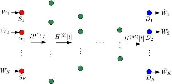
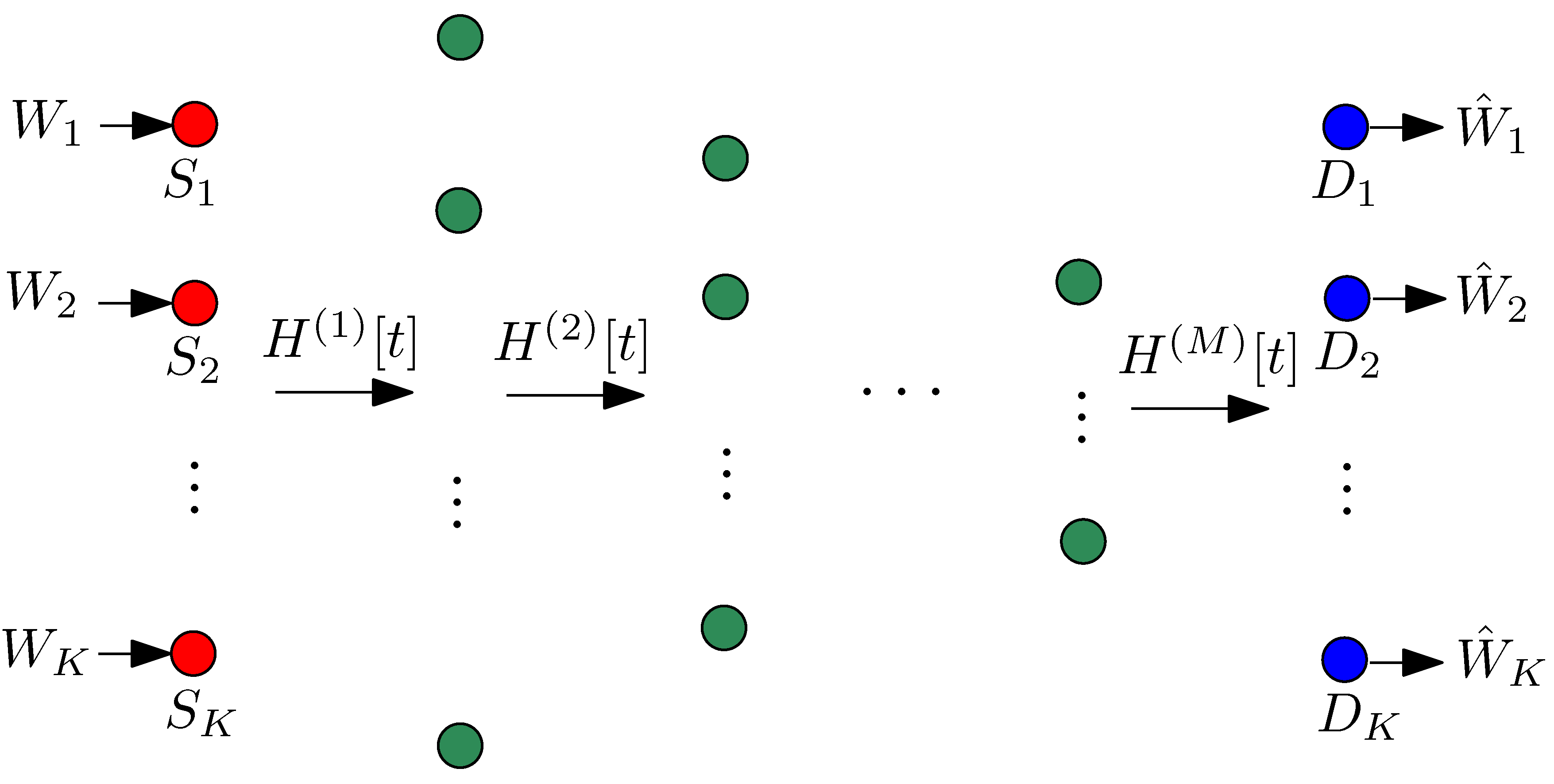
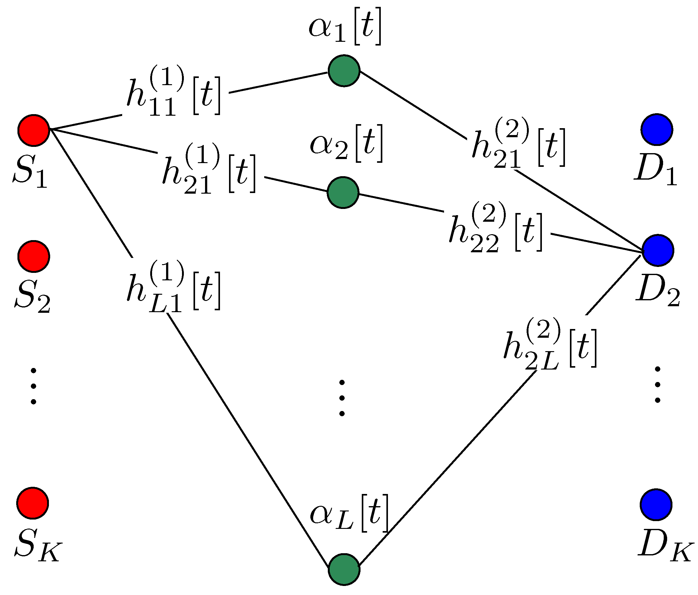
1.3. Layered Multi-Source Multi-Hop Networks

In this subsection, we formally define multi-source multi-hop networks and the degrees of freedom mainly considered in this paper. Of particular interest in this paper is the general layered multi-source multi-hop network depicted in Figure 2. Each source k wishes to send an independent message $W_k$ to destination k over M hop transmission, where $k\in \{1,\cdots ,K\}$. Let $K_m$ denote the number of nodes in each layer, where $m\in \{0,\cdots ,M\}$. The nodes in the 0th layer and the nodes in the Mth layer are the sources and destinations, respectively. That is, $K=K_0=K_M$. For $m\in \{1,\cdots ,M\}$, let $X^{\left(m\right)}\left[t\right]={\left\{x_j^{\left(m\right)}\left[t\right]\right\}}_{j\in \{1,\cdots ,K_{m-1}\}}$ denote the input vector of the set of $K_{m-1}$ nodes in the $(m-1)$th layer at time t and $Y^{\left(m\right)}\left[t\right]={\left\{y_i^{\left(m\right)}\left[t\right]\right\}}_{i\in \{1,\cdots ,K_m\}}$ denote the output vector of the set of $K_m$ nodes in the mth layer at time t. Then the input–output relation of the mth hop at time t is given by

$$Y^{\left(m\right)}\left[t\right]=H^{\left(m\right)}\left[t\right]X^{\left(m\right)}\left[t\right]+Z^{\left(m\right)}\left[t\right]$$

(1)

where $H^{\left(m\right)}\left[t\right]={\left\{h_{ij}^{\left(m\right)}\left[t\right]\right\}}_{i\in \{1,\cdots ,K_m\},j\in \{1,\cdots ,K_{m-1}\}}$ is the complex channel matrix of the mth hop at time t, i.e., the channel matrix from the set of $K_{m-1}$ nodes in the $(m-1)$th layer to the set of $K_m$ nodes in the mth layer, and $Z^{\left(m\right)}\left[t\right]={\left\{z_i^{\left(m\right)}\left[t\right]\right\}}_{i\in \{1,\cdots ,K_m\}}$ is the additive noise vector of the mth hop at time t. We assume that the elements of $Z^{\left(m\right)}\left[t\right]$ are independent and identically distributed (i.i.d.) drawn from the zero-mean and unit-variance circularly symmetric complex Gaussian distribution $\mathcal{CN}(0,1)$. Each node should satisfy the average power constraint P during the transmission, i.e., $\mathsf{E}[|x_j^{\left(m\right)}[t]{|}^2]\le P$ for all $j\in \{1,\cdots ,K_{m-1}\}$ and $m\in \{1,\cdots ,M\}$. Notice that if $M=1$ then the considered model coincides with the K-user interference channel.

Figure 2. Layered multi-source multi-hop networks, where $S_k$ and $D_k$ denote the kth source and its destination, respectively.

Figure 2. Layered multi-source multi-hop networks, where $S_k$ and $D_k$ denote the kth source and its destination, respectively.

Unless otherwise specified, we will assume that the channel coefficients are i.i.d. drawn from a continuous function $f\left(x\right)$, $x\in \mathbb{C}$, and also independent over time. That is, the probability density function of $H^{\left(m\right)}\left[t\right]$ is given as $f_{H^{\left(m\right)}\left[t\right]}\left(H\right)={\prod }_{i,j}f\left(h_{ij}\right)$, where $H=\left\{h_{ij}\right\}$. The channel coefficients are assumed to be revealed to every node in the network.

Throughout the paper, we will deal with the capacity (or approximate capacity) and the degrees of freedom. For this, we briefly introduce the definitions of the achievable rate and achievable degrees of freedom. Let $W_k$ be the message of source k uniformly distributed over $\{1,\cdots ,2^{n{R}_k}\}$, where n denotes the block length. A rate tuple $(R_1,\cdots ,R_K)$ is said to be achievable if there exists a sequence of $(2^{n{R}_1},\cdots ,2^{n{R}_K},n)$ codes such that the probabilities of error for $W_1$ to $W_K$ converge to zero as n increases. For an achievable sum rate ${\sum }_{k=1}^K{R}_k$, the corresponding achievable sum degrees of freedom is defined as

$$\mathsf{DoF}:=\underset{P\to \infty }{lim}\frac{{\sum }_{k=1}^K{R}_k}{logP}$$

(2)

Finally, the sum capacity is defined as the maximum achievable sum rate and the optimal degrees of freedom is the maximum achievable sum degrees of freedom.

Remark 1 (Notation) We will denote matrices or vectors by uppercase letters. We will also denote time-extended matrices and time-extended vectors by boldface uppercase letters and boldface lowercase letters, respectively. Specifically, for a sequence of $\left\{a\right[1],\cdots ,a[T\left]\right\}$, we define $\mathbf{a}:={[a\left[1\right],\cdots ,a\left[T\right]]}^T$ and $\mathbf{A}:=diag\left(a\right[1],\cdots ,a[T\left]\right)$, where ${(·)}^T$ denotes the transpose and $diag\left(a\right[1],\cdots ,a[T\left]\right)$ denotes the diagonal matrix with $a\left[i\right]$ as the $(i,i)$th element.

To describe the ergodic interference alignment and ergodic interference neutralization schemes, we find it convenient to introduce the notation $H\simeq G$ to indicate that the two matrices H and G are almost equal, in the following sense: Consider a long sequence of matrices $H\left[t\right]$, drawn i.i.d. according to a certain probability density function. We partition this long sequence judiciously into pairs of matrices $\left(H\right[t],H[t+\tau \left]\right)$ such that $H[t+\tau ]$ and $F\left(H\right[t\left]\right),$ where $F(·)$ is a cleverly chosen mapping to be discussed below, are almost equal. The main argument is that by considering a longer and longer sequence of matrices, we can make these two matrices arbitrarily close (provided the partitioning into pairs is done optimally). The formal and technical details of this argument can be found in [15].

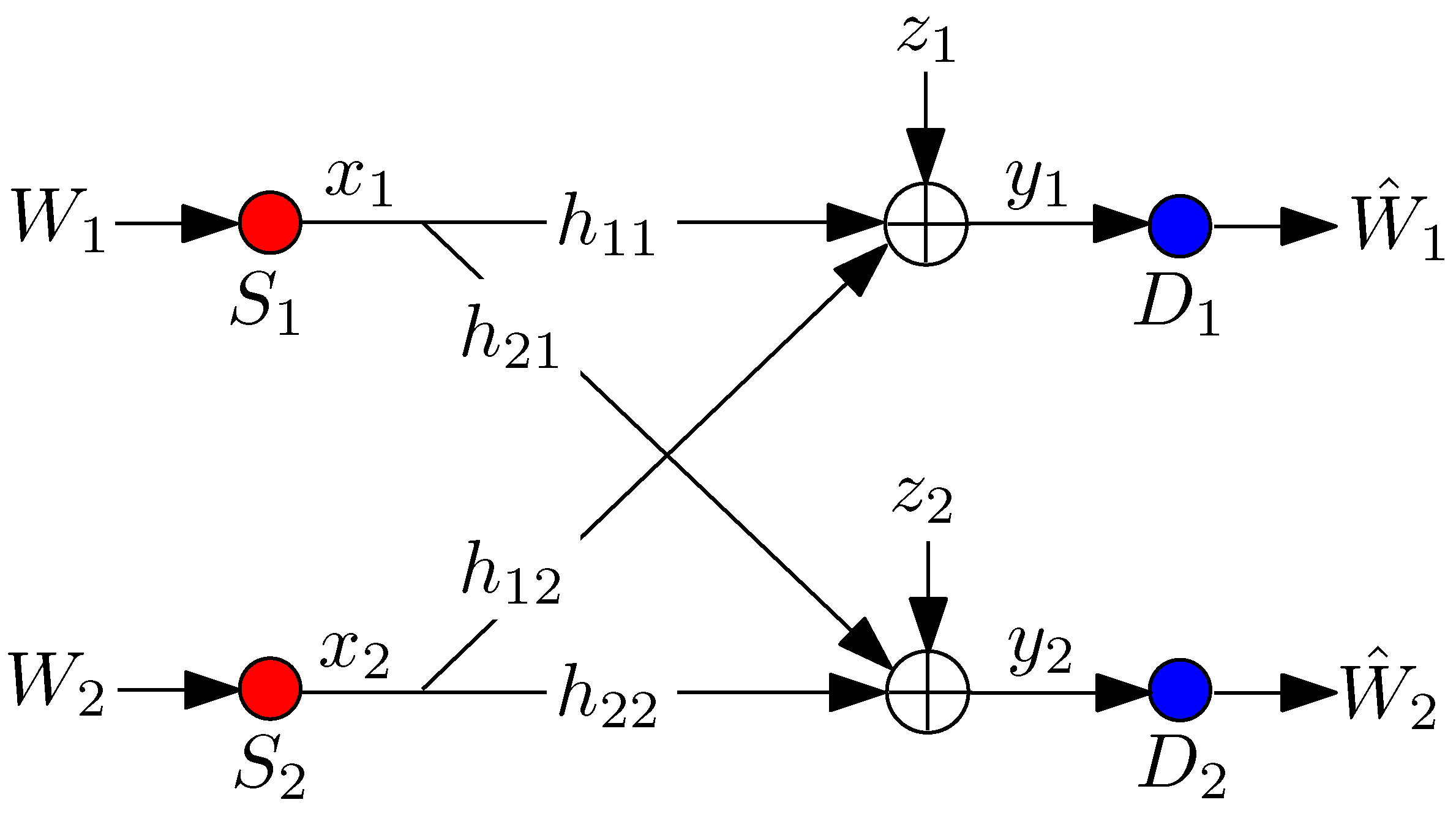
2. Single-Hop Networks: Interference Alignment

In this section, we consider a single-hop network, which corresponds to the case where $M=1$ in Section 1.3. For notational convenience, we will omit the superscript m in Equation (1) if $M=1$. That is, the input–output relation is given by

$$Y\left[t\right]=H\left[t\right]X\left[t\right]+Z\left[t\right]$$

(3)

where $X\left[t\right]=\left\{x_j\left[t\right]\right\}$, $Y\left[t\right]=\left\{y_i\left[t\right]\right\}$, $H\left[t\right]=\left\{h_{ij}\left[t\right]\right\}$, and $Z\left[t\right]=\left\{z_i\left[t\right]\right\}$, which corresponds to the K-user interference channel.

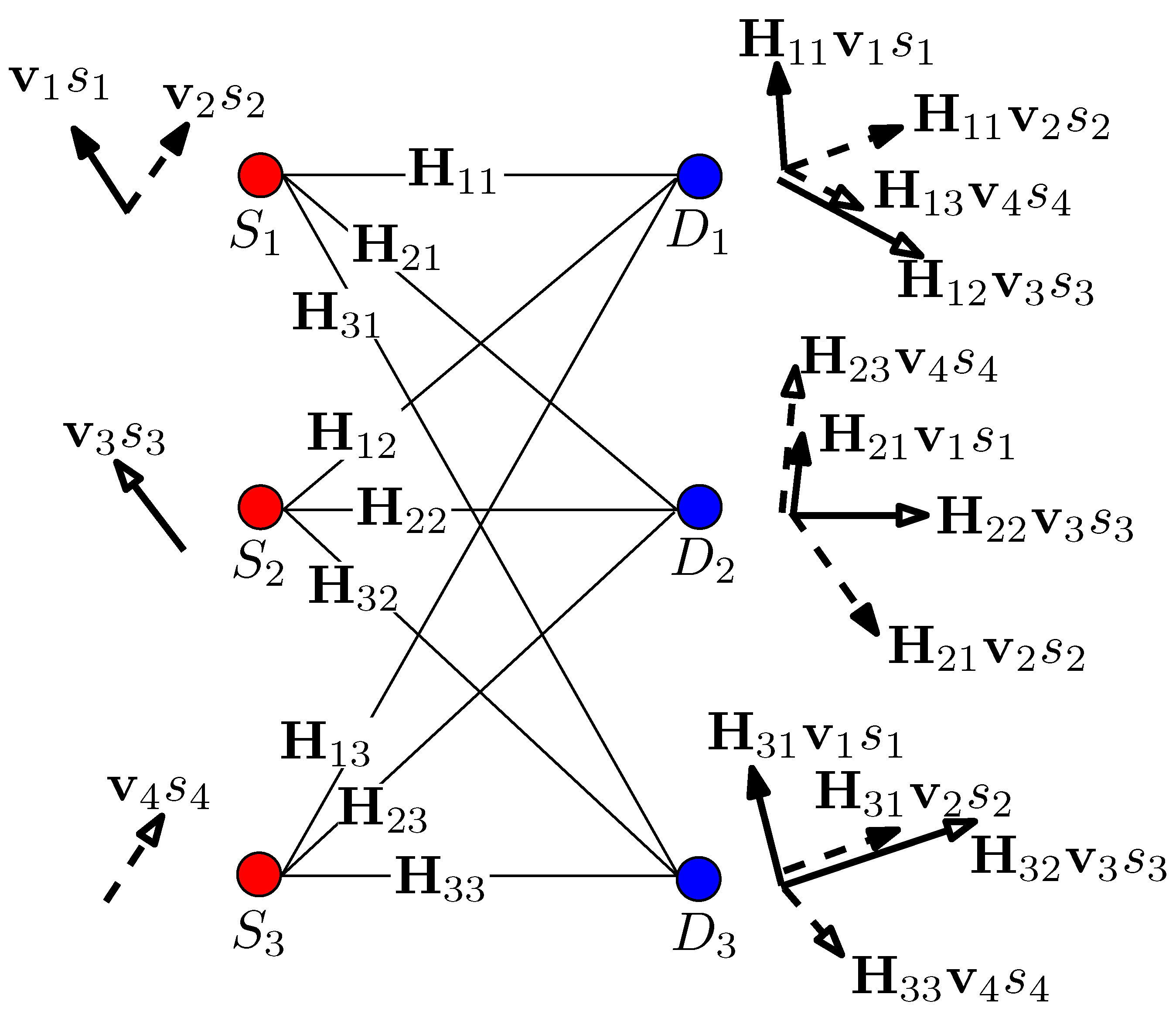
2.1. Signal-Space Interference Alignment

Interference alignment has been observed in the context of the index coding problem [22] and the 2-user X network [7]. A general interference alignment scheme for the K-user interference channel has been developed by Cadambe and Jafar [6] showing that the optimal $\mathsf{DoF}=K/2$ is achievable. The result is quite encouraging since it implies that interference is not a fundamental limiting factor for multi-source single-hop networks.

For a conceptual understanding, consider the 3-user interference channel in Figure 3 in which a transmit signal will be received by each destination with few symbol delay according to its propagation distance (see also [6, Appendix I]). For example, destination 1 will receive the intended signal from source 1 with 2 symbol delay, but will receive the interference signals from sources 2 and 3 with 1 and 3 symbol delays, respectively. Therefore, if each source transmits only using odd time, $t\in \{1,3,5,\cdots \}$, then each destination is able to receive its interference-free intended signal at odd time, since all interference signals from the other sources will arrive only at even time. That is, interference will be aligned within even time and, as a result, each SD pair can achieve $1/2$ degrees of freedom, which provides $\mathsf{DoF}=3/2$. This achievability is strictly better than $\mathsf{DoF}=1$ achievable by time-sharing between SD pairs. Notice that half of the signal dimensions are used for receiving the intended signal and the other half of the signal dimensions are used for aligning $K-1$ interference signals.

The interference alignment technique described above is only possible when the nodes are employed at specific locations, e.g., as shown in Figure 3. In the seminal work [6], Cadambe and Jafar showed that linear interference alignment, i.e., signal space alignment after time extension and linear beamforming, can be done for the general K-user interference channel, which holds almost surely if the channel coefficients are i.i.d. drawn from a continuous function as assumed in Section 1.3. The same principle in the example in Figure 3 can asymptotically be achieved by linear interference alignment as the size of symbol extension increases. That is, almost half of the signal dimensions are used for receiving the intended signal and the rest of the signal dimensions are used for aligning interference at each destination, leading to the fact that $\mathsf{DoF}=K/2$ is achievable.

Figure 3. The 3-user interference channel with propagation delay, where the first dotted circle from each source denotes the distance experiencing one-symbol propagation delay, the second dotted circle denotes the distance experiencing two-symbol propagation delay, etc.

Figure 3. The 3-user interference channel with propagation delay, where the first dotted circle from each source denotes the distance experiencing one-symbol propagation delay, the second dotted circle denotes the distance experiencing two-symbol propagation delay, etc.

To illustrate the strategy of linear interference alignment, we quote an example given in [6, Section III. C], establishing the achievability of $\mathsf{DoF}=4/3$ for the 3-user interference channel with 3 symbol extension. Figure 4 illustrates linear beamforming at each source and the received beams experiencing the channel coefficients at each destination. Here, ${\mathbf{H}}_{ij}$ denotes $diag(h_{ij}\left[1\right],h_{ij}\left[2\right],h_{ij}\left[3\right])$ and ${\mathbf{v}}_l$ denotes the $3\times 1$ transmit beam vector transmitted over $t\in \{1,2,3\}$. To send two symbols $s_1$ and $s_2$, source 1 uses two transmit beams ${\mathbf{v}}_1$ and ${\mathbf{v}}_2$. On the other hand, sources 2 and 3 send $s_3$ and $s_4$ using ${\mathbf{v}}_3$ and ${\mathbf{v}}_4$, respectively. That is, ${\mathbf{x}}_1={\mathbf{v}}_1{s}_1+{\mathbf{v}}_2{s}_2$, ${\mathbf{x}}_2={\mathbf{v}}_3{s}_3$, and ${\mathbf{x}}_3={\mathbf{v}}_4{s}_4$. Therefore, if the following conditions are satisfied, then $s_1$ to $s_4$ can be extracted with nonzero (effective) channel gains:

$$\begin{array}{cc}& {\mathbf{H}}_{12}{\mathbf{v}}_3={\mathbf{H}}_{13}{\mathbf{v}}_4:\text{Interference alignment at destination }1\hfill \end{array}$$

(4a)

$$\begin{array}{cc}& {\mathbf{H}}_{21}{\mathbf{v}}_1={\mathbf{H}}_{23}{\mathbf{v}}_4:\text{Interference alignment at destination }2\hfill \end{array}$$

(4b)

$$\begin{array}{cc}& {\mathbf{H}}_{31}{\mathbf{v}}_2={\mathbf{H}}_{32}{\mathbf{v}}_3:\text{Interference alignment at destination }3\hfill \end{array}$$

(4c)

$$\begin{array}{cc}\hfill span({\mathbf{H}}_{11}{\mathbf{v}}_1& ,{\mathbf{H}}_{11}{\mathbf{v}}_2,{\mathbf{H}}_{12}{\mathbf{v}}_3)={\mathbb{C}}^{3\times 3}:\text{Linearly independence at destination }1\hfill \end{array}$$

(4d)

$$\begin{array}{cc}\hfill span({\mathbf{H}}_{21}{\mathbf{v}}_1& ,{\mathbf{H}}_{21}{\mathbf{v}}_2,{\mathbf{H}}_{22}{\mathbf{v}}_3)={\mathbb{C}}^{3\times 3}:\text{Linearly independence at destination }2\hfill \end{array}$$

(4e)

$$\begin{array}{cc}\hfill span({\mathbf{H}}_{31}{\mathbf{v}}_1& ,{\mathbf{H}}_{31}{\mathbf{v}}_2,{\mathbf{H}}_{33}{\mathbf{v}}_4)={\mathbb{C}}^{3\times 3}:\text{Linearly independence at destination }3\hfill \end{array}$$

(4f)

where $span(·)$ denotes the vector space spanned by a set of vectors.

For an arbitrarily chosen ${\mathbf{v}}_3$, we can set

$$\begin{array}{cc}\hfill {\mathbf{v}}_4& ={{\mathbf{H}}_{13}}^{-1}{\mathbf{H}}_{12}{\mathbf{v}}_3\hfill \end{array}$$

(5a)

$$\begin{array}{cc}\hfill {\mathbf{v}}_1& ={{\mathbf{H}}_{21}}^{-1}{\mathbf{H}}_{23}{\mathbf{v}}_4={{\mathbf{H}}_{21}}^{-1}{\mathbf{H}}_{23}{{\mathbf{H}}_{13}}^{-1}{\mathbf{H}}_{12}{\mathbf{v}}_3\hfill \end{array}$$

(5b

$$\begin{array}{cc}\hfill {\mathbf{v}}_2& ={{\mathbf{H}}_{31}}^{-1}{\mathbf{H}}_{32}{\mathbf{v}}_3\hfill \end{array}$$

(5c)

which satisfy the alignment conditions (4a) to (4c). Since the beamforming vectors were set independent of the direct channel matrices ${\mathbf{H}}_{11}$, ${\mathbf{H}}_{22}$, and ${\mathbf{H}}_{33}$, we can guarantee almost surely that ${\mathbf{H}}_{12}{\mathbf{v}}_3\notin span({\mathbf{H}}_{11}{\mathbf{v}}_1,{\mathbf{H}}_{11}{\mathbf{v}}_2)$, ${\mathbf{H}}_{22}{\mathbf{v}}_3\notin span({\mathbf{H}}_{21}{\mathbf{v}}_1,{\mathbf{H}}_{21}{\mathbf{v}}_2)$, and ${\mathbf{H}}_{33}{\mathbf{v}}_4\notin span({\mathbf{H}}_{31}{\mathbf{v}}_1,{\mathbf{H}}_{31}{\mathbf{v}}_2)$ for genetic channel coefficients, i.e., when the channel coefficients are i.i.d. drawn from a continuous distribution. Similarly, ${\mathbf{v}}_1$ and ${\mathbf{v}}_2$ in Equations (5b) and (5c) are linearly independent almost surely, which leads to ${\mathbf{H}}_{11}{\mathbf{v}}_1\notin span\left({\mathbf{H}}_{11}{\mathbf{v}}_2\right)$, ${\mathbf{H}}_{21}{\mathbf{v}}_1\notin span\left({\mathbf{H}}_{21}{\mathbf{v}}_2\right)$, and ${\mathbf{H}}_{31}{\mathbf{v}}_1\notin span\left({\mathbf{H}}_{31}{\mathbf{v}}_2\right)$ almost surely. Therefore, we can guarantee almost surely that the beamforming vectors in Equations (5a)–(5c) also satisfy the linearly independence conditions in Equations (4d)–(4f).

Figure 4. Linear interference alignment for the 3-user interference channel with 3 symbol extension.

Figure 4. Linear interference alignment for the 3-user interference channel with 3 symbol extension.

Although the above example shows that $\mathsf{DoF}=4/3$ is achievable with 3 symbol extension for the 3-user interference channel, it is still hard to capture the main idea of achieving the optimal $\mathsf{DoF}=3/2$, as the size of symbol extension increases by this example. For the general K-user interference channel, Cadambe and Jafar proposed linear interference alignment and showed that the optimal $\mathsf{DoF}=K/2$ is asymptotically achievable as the size of symbol extension increases. We refer to [6, Appendix III] for the detailed proof.

Remark 2 (Extensions) Linear interference alignment has been widely and successfully adapted to the interference channel with multiple antennas [9], cooperation [12,13], general message demand [8,14], etc. It also has potential for distributed storage problem [23,24] and index coding problem [25].

Remark 3 (Complexity and Delay) For the K-user interference channel, the optimal $\mathsf{DoF}=K/2$ is achievable as the size of symbol extension T tends to infinity. Specifically,

$$\mathsf{DoF}=\frac{{(T+1)}^N+(K-1)T^N}{{(T+1)}^N+T^N}$$

(6)

is achievable with T symbol extension, where $N=(K-1)(K-2)-1$ [6, Appendix III]. In practice, however, due to the system complexity and delay, it is hard to let T be arbitrarily large and, thus, the rate of convergence in Equation (6) to the optimal $K/2$ can be critical for practical systems. Choi et al. [26] addressed this issue and proposed another beamforming design that improves the convergence rate of Equation (6).

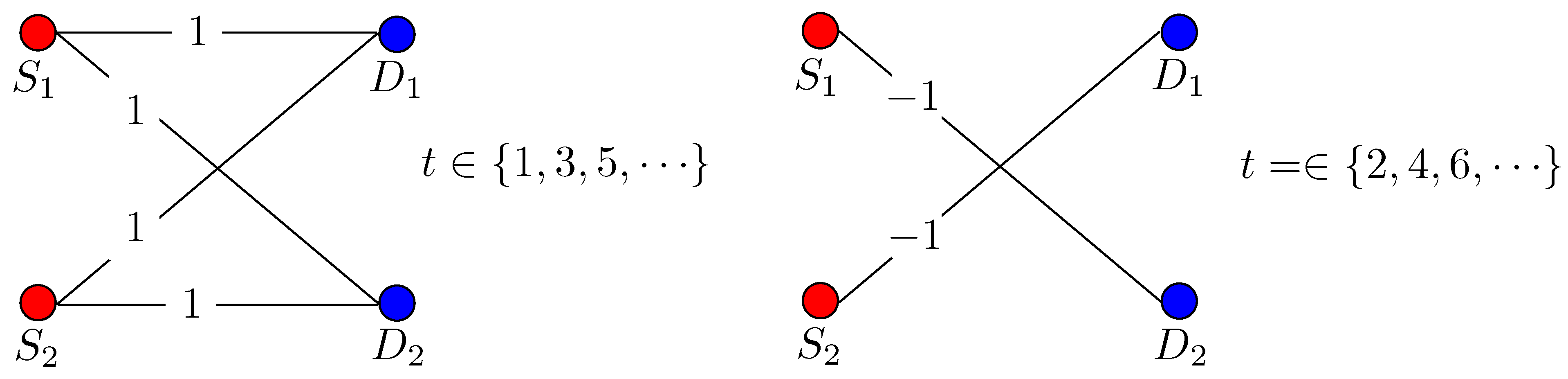
2.2. Ergodic Interference Alignment

The K-user interference channel with time-varying channel coefficients, which corresponds to the network in Section 1.3 with $M=1$, is in general non-separable [27,28]. This means that coding jointly over multiple channel states can generally outperform coding separately in each individual channel state. For instance, suppose the 2-user inference channel in Figure 5 in which

$$H\left[t\right]=\left\{\begin{array}{cc}\left[\begin{array}{cc}1& 1\\ 1& 1\end{array}\right]\hfill & \text{for }t\in \{1,3,5,\cdots \}\hfill \\ \left[\begin{array}{cc}0& -1\\ -1& 0\end{array}\right]\hfill & \text{for }t\in \{2,4,6,\cdots \}\hfill \end{array}\right.$$

(7)

If we apply coding for odd time and even time separately, then it is immediately clear that we have the upper bound $\mathsf{DoF}\le 1/2:$ the rank of $H\left[t\right]$ is one for odd t (thus one degree of freedom is achievable for this channel state) and the direct channel coefficients in $H\left[t\right]$ are zeros for even t (thus zero degree of freedom is achievable for this channel state). However, by transmitting the same signal twice over two adjacent time indices, i.e., $X\left[1\right]=X\left[2\right]$ and $X\left[3\right]=X\left[4\right]$, and so on, interference can first be decoded at each destination based on $\left\{Y\right[2],Y[4],\cdots \}$ and its effect can then be subtracted in $\left\{Y\right[1],Y[3],\cdots \}$. Then each destination can decode its message from the interference-free received signals $\{Y^{\prime }\left[1\right],Y^{\prime }\left[3\right],\cdots \}$. This simple joint coding scheme achieves a rate of $\frac{1}{2}{log}_2(1+P)$ for each SD pair, proving that we can attain $\mathsf{DoF}=1$. Therefore, this joint coding scheme is strictly better than any separation-based coding scheme.

Figure 5. Example of the 2-user interference channel having two channel states.

Figure 5. Example of the 2-user interference channel having two channel states.

There is a second interesting observation concerning this simple example. Namely, if each receiver simply adds up two adjacent received signals, i.e., $Y\left[1\right]+Y\left[2\right]$, $Y\left[3\right]+Y\left[4\right]$, and so on, we observe that the interference directly disappears. This is due to the fact that in our simple example, $H\left[t\right]+H[t+1]$ is the identity matrix.

This idea can be pushed further, leading to the concept of ergodic interference alignment. For the K-user finite field interference channel (with time-varying channel coefficients), this was independently proposed by Nazer et al. [29] and Jeon and Chung [30] in two slightly different versions. When the channel coefficients are drawn from a continuous function (such as, for example, Rayleigh fading), it is not immediately clear that one can again align channel matrices as in the above simple example. Nevertheless, using a channel quantization argument, for the K-user Gaussian interference channel (with time-varying channel coefficients), Nazer et al. [15,29] showed the achievability of

$$R_k=\frac{1}{2}\mathsf{E}[log(1+2|h_{kk}{\left[t\right]|}^{2}P\left)\right]$$

(8)

for all $k\in \{1,\cdots ,K\}$, where the expectation is taken over the channel coefficients. To explain the achievability, for a given channel state $H=\left\{h_{ij}\right\}$, define $F\left(H\right)=\left\{f_{ij}\right\}$ such that $f_{ij}=h_{ij}$ if $i=j$ and $f_{ij}=-h_{ij}$ if $i\ne j$ for all $i,j\in \{1,\cdots ,K\}$. Therefore,

$$H+F\left(H\right)=diag(2h_{11},2h_{22},\cdots ,2h_{KK})$$

(9)

The same principle explained in Figure 5 can be applied by transmitting the same signal twice through two particularly paired channel states, approximately given by H and $F\left(H\right)$. Suppose that the sources transmit $X\left[t\right]$ at time t. The sources transmit $X\left[t\right]$ repeatedly with an appropriate delay τ, i.e., $X[t+\tau ]=X\left[t\right]$, such that $H[t+\tau ]$ is approximately given as $H[t+\tau ]\simeq F\left(H\right[t\left]\right)$. Then the destinations add two received signals $Y\left[t\right]$ and $Y[t+\tau ]$, which gives

$$\begin{array}{cc}\hfill Y\left[t\right]+Y[t+\tau ]& \simeq \left(H\right[t]+F(H\left[t\right]\left)\right)X\left[t\right]+Z\left[t\right]+Z[t+\tau ]\hfill \end{array}$$

$$\begin{array}{cc}& =diag(2h_{11}\left[t\right],2h_{22}\left[t\right],\cdots ,2h_{KK}\left[t\right])X\left[t\right]+Z\left[t\right]+Z[t+\tau ]\hfill \end{array}$$

(10)

In order to utilize almost all channel instances for transmission, the probability density functions between two paired channels should be the same. That is,

$$f_{H\left[t\right]}\left(H\right)=f_{H\left[t\right]}\left(F\left(H\right)\right)$$

(11)

should be satisfied for all $H\in {\mathbb{C}}^{K\times K}$. Under i.i.d. channel coefficients as assumed in Section 1.3, this condition is satisfied if $f\left(h\right)=f(-h)$ for all $h\in \mathbb{C}$, which holds for a broad class of channel distributions. Therefore, assuming that $f\left(h\right)=f(-h)$, almost all channel realizations can be utilized for this ergodic pairing as the block length n increases. More specifically, this statement can be verified by quantization of channel space and then pairing quantized channel spaces based on the function $F\left(H\right)$. From the strong typicality, the numbers of channel instances belonging to the paired quantized channel spaces are almost the same as the block length n increases, since Equation (11) are the same for all $H\in {\mathbb{C}}^{K\times K}$. For the rigorous proof, we need to carefully consider channel quantization and randomness of channel realizations. We omit the detailed proof here and refer to [15, Theorem 2]. From Equation (10), the signal-to-noise-interference ratio (SINR) at destination k is approximately given by $\frac{4|h_{kk}{\left[t\right]|}^{2}P}{2}=2{\left|h_{kk}\left[t\right]\right|}^{2}P$. Hence we can show that Equation (8) is achievable.

Remark 4 (Approximate Ergodic Capacity) From Equation (8), this new coding strategy provides at least $1/2$ of its interference-free ergodic capacity at any P since it makes interference aligned at a finite P. This property leads to characterize the ergodic capacity to within a constant number of bits/sec/Hz for some important class of channel distributions, which will be discussed in Section 4.1.

Remark 5 (Extensions) Ergodic interference alignment has been extended to a certain class of general message demand and 2-user X channel (see [15, Theorems 4,5]). It can also be applied to communication with secrecy constraints [31].

Remark 6 (Complexity and Delay) For ergodic interference alignment, even though the transmission itself is a simple repeated transmission with some delay, ergodic pairing of channel instances satisfying arbitrarily small quantization error requires unbounded buffer or storage at each node and also causes unbounded delay. The work [32] studied a delay–rate trade-off achievable by ergodic interference alignment and also modified the original ergodic interference alignment scheme [15] to enhance the delay–rate trade-off.

2.3. Other Interference Alignment Techniques

We have discussed two recently developed techniques to attain interference alignment. Both techniques rely on time-varying channel coefficients in order to obtain a sufficiently rich environment to allow aligning the interference signals. Other techniques have also been studied in the literature.

Most notably, it was shown that interference alignment can also be attained on fixed (not time-varying) interference channels. In [33], asymmetric complex signaling has been used to show that $\mathsf{DoF}=6/5$ and $\mathsf{DoF}=4/3$ are achievable for the 3-user interference channel and 2-user X channel respectively. It was shown later that for the general K-user interference channel, the optimal $\mathsf{DoF}=K/2$ is achieved via a framework using rational dimensions, i.e., signal scaling alignment, and we refer to [34,35] for details.

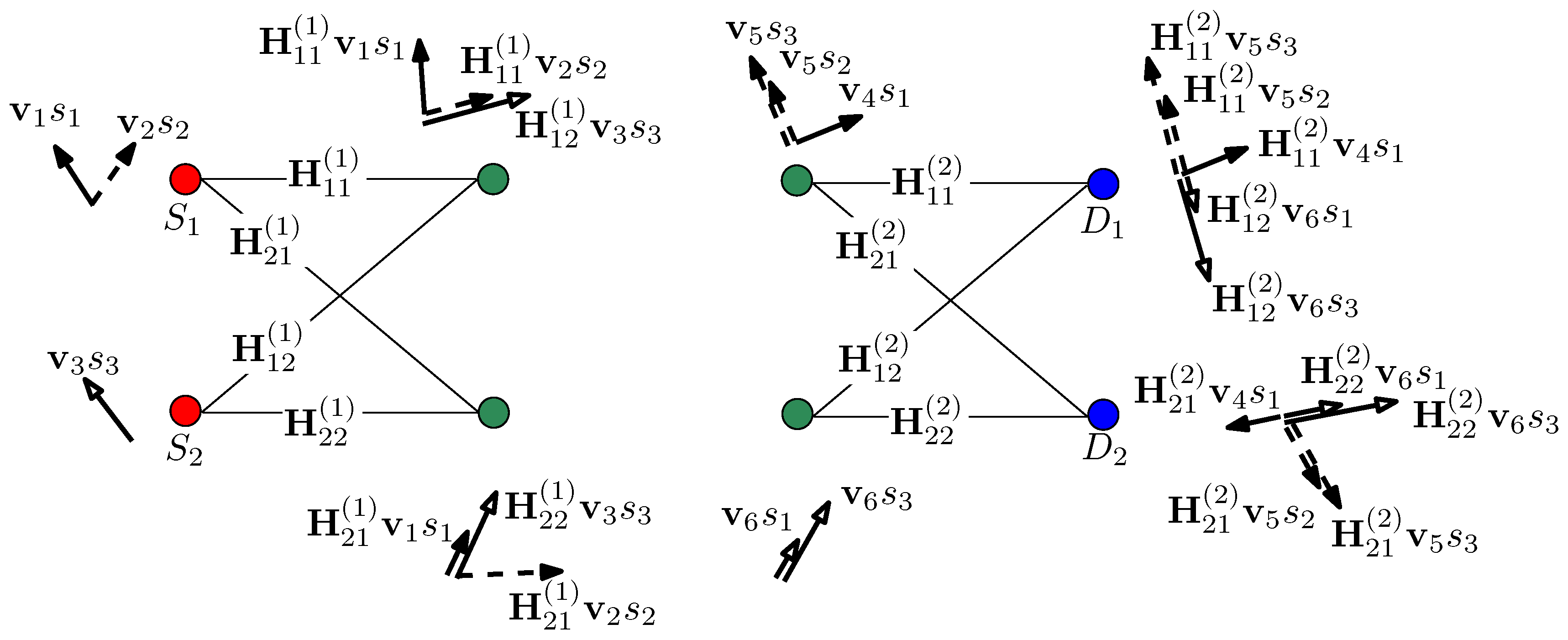
3. Multi-Hop Networks: Interference Neutralization

In this section, we consider multi-hop networks of the type defined in Section 1.3 (with $M\ge 2$). For multi-source multi-hop networks, interference can be cancelled by aligning multiple paths through a network, a technique referred to as interference neutralization. Proper use of such interference neutralization is the key for an approximate capacity [17] and the degrees of freedom characterization [18,19] of multi-source multi-hop networks.

Figure 6 illustrates the general two-hop network, i.e., $M=2$ with $K_0=K_2=K$ and $K_1=L$ in Section 1.3. Assume that relay i amplifies its received signal $y_i^{\left(1\right)}\left[t\right]$ with amplification factor ${\alpha }_i\left[t\right]$ and forwards it to the destinations as shown in Figure 6. That is, $x_i^{\left(2\right)}\left[t\right]={\alpha }_i\left[t\right]y_i^{\left(1\right)}\left[t\right]$. Then, the interference from source 1 to destination 2 is neutralized if we choose the coefficients $\left\{{\alpha }_i\left[t\right]\right\}$ such that

$$\sum _{i=1}^L{h}_{2i}^{\left(2\right)}\left[t\right]{\alpha }_i\left[t\right]h_{i1}^{\left(1\right)}\left[t\right]=0$$

(12)

is satisfied. We note that this is a linear equation with respect to the coefficients $\left\{{\alpha }_i\left[t\right]\right\}$. Now, clearly, it is not sufficient to only neutralize the interference from source 1 to destination 2. Rather, we want to completely neutralize all interference from every source to every destination. This leads to $K(K-1)$ linear constraints of the above form. There are L coefficients $\left\{{\alpha }_i\left[t\right]\right\}.$ Hence, to neutralize all interference in this direct fashion, a necessary condition is $L\ge K(K-1),$ and a sufficient condition is $L\ge K(K-1)+1.$ Thus, if $L\ge K(K-1)+1$, we can find nonzero $\left\{{\alpha }_i\left[t\right]\right\}$ to neutralize all the interference by amplify-and-forward relaying [16]. Thus, as long as the resulting equivalent gains from each source to its corresponding destination are nonzero for this choice of coefficients, we can attain K degrees of freedom. It is also clear that it is not possible to attain more than K degrees of freedom, and thus, this is optimal in a degree-of-freedom sense.

Figure 6. Amplify-and-forward-based interference neutralization for two-hop networks.

Figure 6. Amplify-and-forward-based interference neutralization for two-hop networks.

What to do if the number of relays L is comparable to the number of SD pairs $K,$ hence $L<K(K-1)+1$? In this case, it is impossible to select the coefficients $\left\{{\alpha }_i\left[t\right]\right\}$ in such a way as to neutralize all interference. More precisely, it is not difficult to show that in general, for the above strategy, any choice of the coefficients $\left\{{\alpha }_i\left[t\right]\right\}$ will lead to a number of degrees of freedom that is strictly smaller than $K.$ We note that a simple cut-set upper bound for the general two-hop network in Figure 6 evaluates to K degrees of freedom as long as $L\ge K,$ and thus, one interesting question is whether there is a different strategy that can attain K degrees of freedom. The general answer to this question is open, but for some important classes of networks, the optimal $\mathsf{DoF}=K$ is achievable using the recently developed aligned interference neutralization and ergodic interference neutralization techniques [18,19]. This is explained in detail in the following two subsections.

3.1. Neutralization with Symbol Extension

Let us now consider the special case where $M=2$ with $K_0=K_1=K_2=2$ in Section 1.3. This model is also referred to as the $2\times 2\times 2$ network in the literature. For this network, the cut-set bound evaluates to 2 degrees of freedom, yet the simple strategy outlined above does not permit to completely neutralize interference, and hence, fails to attain 2 degrees of freedom. More specifically, with reference to Figure 6, in order to neutralize interference completely, we need to choose the coefficients $\left\{{\alpha }_i\left[t\right]\right\}$ to satisfy

$$\begin{array}{c}\hfill h_{21}^{\left(1\right)}\left[t\right]{\alpha }_1\left[t\right]h_{11}^{\left(1\right)}\left[t\right]+h_{22}^{\left(1\right)}\left[t\right]{\alpha }_2\left[t\right]h_{21}^{\left(1\right)}\left[t\right]=0\end{array}$$

$$\begin{array}{c}\hfill h_{11}^{\left(1\right)}\left[t\right]{\alpha }_1\left[t\right]h_{12}^{\left(1\right)}\left[t\right]+h_{12}^{\left(1\right)}\left[t\right]{\alpha }_2\left[t\right]h_{22}^{\left(1\right)}\left[t\right]=0\end{array}$$

(13)

which are two linear equations with two variables, ${\alpha }_1\left[t\right]$ and ${\alpha }_2\left[t\right]$. For generic channel coefficients, however, ${\alpha }_1\left[t\right]={\alpha }_2\left[t\right]=0$ is the only solution that satisfies Equation (13), which prevents communication completely.

Progress can be made by considering so-called symbol extension, by which we mean that we do not treat every time instant the same, and that the coefficients $\left\{{\alpha }_i\left[t\right]\right\}$ are allowed to vary over time. Specifically, it was shown in [18, Section III. D] that the optimal $\mathsf{DoF}=2$ is asymptotically achievable for the $2\times 2\times 2$ network by symbol extension and as the size of symbol extension increases. In particular, we combine T consecutive channel inputs into a “supersymbol” and apply a generalized amplify-and-forward relaying strategy at relay i by setting ${\mathbf{x}}_i^{\left(1\right)}=A_i{\mathbf{y}}_i^{\left(1\right)}$, where $A_i$ denotes the $T\times T$ matrix consisting of $T^2$ amplification factors (the coefficients $\left\{{\alpha }_i\left[t\right]\right\}$ of the relay for the T channel uses). The main trick is now that source 1 sends T symbols with arbitrarily chosen T transmit beams (vectors of length T), but source 2 only sends $T-1$ symbols using $T-1$ arbitrarily chosen transmit beams (vectors of length T). Thus, a total of $2T-1$ symbols is transmitted over T channel uses. As we will now show, all of these $2T-1$ symbols are received without any interference by their respective receivers. Specifically, in order to avoid interference, we have to satisfy $T^2+T(T-1)$ equations that are linear in terms of the entries of the two matrices of relaying coefficients $A_1$ and $A_2.$ However, these matrices have a total of $2T^2$ entries that can be selected freely, and since $2T^2>T^2+T(T-1),$ we are guaranteed to have a solution that leads to complete interference neutralization (except in the case of degenerate channel coefficients, but in that case, the cut-set bound can also be tightened; we omit a more detailed discussion of this less interesting case here). Therefore $\mathsf{DoF}=\frac{2T-1}{T}$ is achievable via symbol extension of length T, and hence, ${lim}_{T\to \infty }\mathsf{DoF}=2$ is achievable in the limit.

A more systematic way of interference neutralization with symbol extension has also been proposed in [18, Section III. A], referred to as aligned interference neutralization. The underlying technique is linear interference alignment introduced in Section 2.1, but the purpose of interference alignment is to neutralize interference at the destinations. To explain the notion of aligned interference neutralization, we quote an example given in [18, Section I. E] achieving $\mathsf{DoF}=3/2$ with 2 symbol extension, which is illustrated in Figure 7. Source 1 sends two symbols $s_1$ and $s_2$ using two transmit beams ${\mathbf{v}}_1$ and ${\mathbf{v}}_2$ and source 2 sends one symbol $s_3$ using ${\mathbf{v}}_3$. For an arbitrarily chosen ${\mathbf{v}}_{\mathbf{3}}$, setting ${\mathbf{v}}_2={({\mathbf{H}}_{11}^{(1)})}^{-1}{\mathbf{H}}_{12}^{\left(1\right)}{\mathbf{v}}_3$ and ${\mathbf{v}}_1={({\mathbf{H}}_{21}^{(1)})}^{-1}{\mathbf{H}}_{22}^{\left(1\right)}{\mathbf{v}}_3$ provides interference alignment in Figure 7 at the end of the first hop:

$$\begin{array}{cc}\hfill {\mathbf{H}}_{11}^{\left(1\right)}{\mathbf{v}}_2& ={\mathbf{H}}_{12}^{\left(1\right)}{\mathbf{v}}_3:\text{Interference alignment at relay }1\hfill \end{array}$$

$$\begin{array}{cc}\hfill {\mathbf{H}}_{21}^{\left(1\right)}{\mathbf{v}}_1& ={\mathbf{H}}_{22}^{\left(1\right)}{\mathbf{v}}_3:\text{Interference alignment at relay }2\hfill \end{array}$$

(14)

Hence, after the first hop, relay 1 can extract $s_1$ and $s_2+s_3$ and relay 2 can extract $s_2$ and $s_1+s_3$. Then relay 1 sends $s_1$ and $s_2+s_3$ using ${\mathbf{v}}_4$ and ${\mathbf{v}}_5$ and relay 2 sends $s_1+s_3$ using ${\mathbf{v}}_6$. Again, for an arbitrarily chosen ${\mathbf{v}}_6$, setting ${\mathbf{v}}_5=-{({\mathbf{H}}_{11}^{\left(2\right)})}^{-1}{\mathbf{H}}_{12}^{\left(2\right)}{\mathbf{v}}_6$ and ${\mathbf{v}}_4=-{({\mathbf{H}}_{21}^{\left(2\right)})}^{-1}{\mathbf{H}}_{22}^{\left(2\right)}{\mathbf{v}}_6$ provides interference neutralization in Figure 7 at the end of the second hop:

$$\begin{array}{cc}\hfill {\mathbf{H}}_{11}^{\left(2\right)}{\mathbf{v}}_5& =-{\mathbf{H}}_{12}^{\left(2\right)}{\mathbf{v}}_6:\text{Interference neutralization at destination }1\hfill \end{array}$$

$$\begin{array}{cc}\hfill {\mathbf{H}}_{21}^{\left(2\right)}{\mathbf{v}}_4& =-{\mathbf{H}}_{22}^{\left(2\right)}{\mathbf{v}}_6:\text{Interference neutralization at destination }2\hfill \end{array}$$

(15)

Therefore, destination 1 can extract $s_1$ and $s_2$ and destination 2 can extract $s_3$ with nonzero (effective) channel gains and $\mathsf{DoF}=3/2$ is achievable.

Figure 7. Aligned interference neutralization for the $2\times 2\times 2$ network with 2 symbol extension.

Figure 7. Aligned interference neutralization for the $2\times 2\times 2$ network with 2 symbol extension.

For the general $2\times 2\times 2$ network, Gou et al. proposed aligned interference neutralization and showed the optimal $\mathsf{DoF}=2$ is asymptotically achievable as the size of symbol extension increases. We refer to [18, Section III. A] for the detailed proof.

Remark 7 (Extensions) Interference neutralization with symbol extension has been extended to the general 2-user network [36] and 2-user X network [37], and also to the case of multi-antenna nodes [38]. However, for generic channel coefficients, the optimal degrees of freedom characterization is in general open for more than two users. For instance, for the model defined in Section 1.3 with $M=2$ with $K_0=K_1=K_2=3$, also referred to as the $3\times 3\times 3$ network, the optimal $\mathsf{DoF}$ is still unknown.

3.2. Ergodic Interference Neutralization

To start our discussion of ergodic interference neutralization, we observe that multi-hop networks consisting of multiple SD pairs are in general non-separable. This should not come as a surprise and parallels our observation for single-hop networks. For instance, consider the $2\times 2\times 2$ network in Figure 8 in which

$$H^{\left(1\right)}\left[t\right]=\left[\begin{array}{cc}1& 0\\ 0& 1\end{array}\right]\text{and }{H}^{\left(2\right)}\left[t\right]=\left[\begin{array}{cc}1& 1\\ 1& 0\end{array}\right]\text{for }t\in \{1,3,5,\cdots \}$$

(16)

and

$$H^{\left(1\right)}\left[t\right]=\left[\begin{array}{cc}0& 1\\ 1& -1\end{array}\right]\text{and }{H}^{\left(2\right)}\left[t\right]=\left[\begin{array}{cc}1& 0\\ 0& 1\end{array}\right]\text{for }t\in \{2,4,6,\cdots \}$$

(17)

If we apply coding for odd times and even times separately, then the achievable degrees of freedom cannot exceed $\mathsf{DoF}\le 1:$ there is no path from source 2 to destination 2 at odd time and from source 1 to destination 1 at even time. By contrast, if we code over both channel instances, we can attain $\mathsf{DoF}=2,$ which is optimal. To see how we can achieve this performance, we simply let the relays amplify and forward their received signals with one symbol delay, i.e., $X^{\left(2\right)}[t+1]=\alpha \left[t\right]Y^{\left(1\right)}\left[t\right]$. That way, interference can completely be neutralized at each destination since

$$H^{\left(2\right)}[t+1]\left[\begin{array}{cc}\alpha \left[t\right]& 0\\ 0& \alpha \left[t\right]\end{array}\right]H^{\left(1\right)}\left[t\right]=\alpha \left[t\right]\left[\begin{array}{cc}1& 0\\ 0& 1\end{array}\right]$$

(18)

for any $\alpha \left[t\right]>0$ satisfying the power constraint P. Therefore, the optimal $\mathsf{DoF}=2$ is achievable for this case.

Figure 8. Example of the $2\times 2\times 2$ network having two channel states.

Figure 8. Example of the $2\times 2\times 2$ network having two channel states.

Under i.i.d. isotropic fading, Jeon et al. showed in [19] that the optimal $\mathsf{DoF}=K$ is achievable for K-user K-hop networks with K relays in each layer, i.e., $M=K$ and $K_m=K$ for all $m\in \{1,\cdots ,K\}$ in Section 1.3. This class of channel distributions includes i.i.d. uniform phase fading and i.i.d. Rayleigh fading as a special case. The basic concept of ergodic interference neutralization is similar to the previous example in Figure 8. Suppose that the sources transmit at time $t_1$. For $m\in \{2,\cdots ,K\}$, the relay nodes in the mth hop transmission amplify and forward the corresponding received signal with an appropriate delay $t_m-t_{m-1}>0$ such that the matrix product

$$H^{\left(K\right)}\left[t_K\right]\cdots H^{\left(2\right)}\left[t_2\right]H^{\left(1\right)}\left[t_1\right]$$

(19)

becomes approximately a diagonal matrix with nonzero diagonal elements, which means that interference is neutralized at each destination. For i.i.d. isotropic fading, a novel ergodic pairing satisfying this condition has been proposed in [19] based on the unordered singular value decomposition.

To explain the notion of the proposed ergodic interference neutralization in [19], consider the case where $K=3$, i.e., the $3\times 3\times 3\times 3$ network. Denote the unordered singular value decomposition of $H\in {\mathbb{C}}^{3\times 3}$ as $S\left(H\right):=(U,\Sigma ,V)$, where U is the $3\times 3$ left unitary matrix, Σ is the $3\times 3$ diagonal matrix with unordered singular values, and V is the $3\times 3$ right unitary matrix. Then H can be represented as $H=U\Sigma V^{†}$, where ${(·)}^{†}$ denotes the complex conjugate transpose. Figure 9 illustrates the ergodic pairing rule proposed in [19]. Suppose that the sources transmit at time $t_1$ and $S\left(H^{\left(1\right)}\left[t_1\right]\right)=(U,diag({\lambda }_1,{\lambda }_2,{\lambda }_3),V)$. The relays in the second hop amplify and forward at an appropriate time $t_2$ such that $S\left(H^{\left(2\right)}\left[t_2\right]\right)\simeq (W,diag({\lambda }_2,{\lambda }_3,{\lambda }_1),U)$, where W can be chosen as any arbitrary unitary matrix. Then the relays in the last hop amplify and forward at an appropriate time $t_3$ such that $S\left(H^{\left(3\right)}\left[t_3\right]\right)\simeq (V,diag({\lambda }_3,{\lambda }_1,{\lambda }_2),W)$. This ergodic pairing satisfies

$$\begin{array}{cc}\hfill H^{\left(3\right)}\left[t_3\right]H^{\left(2\right)}\left[t_2\right]H^{\left(1\right)}\left[t_1\right]& \simeq V\left[\begin{array}{ccc}{\lambda }_3& 0& 0\\ 0& {\lambda }_1& 0\\ 0& 0& {\lambda }_2\end{array}\right]W^{†}W\left[\begin{array}{ccc}{\lambda }_2& 0& 0\\ 0& {\lambda }_3& 0\\ 0& 0& {\lambda }_1\end{array}\right]U^{†}U\left[\begin{array}{ccc}{\lambda }_1& 0& 0\\ 0& {\lambda }_2& 0\\ 0& 0& {\lambda }_3\end{array}\right]V^{†}\hfill \end{array}$$

$$\begin{array}{cc}& =\left({\lambda }_1{\lambda }_2{\lambda }_3\right)I,\hfill \end{array}$$

(20)

where I denotes the identity matrix. Therefore, this pairing satisfies the previous interference neutralization condition. Notice that the probability density functions of the paired channel states are the same for i.i.d. isotropic fading since in this case, $f_{H^{\left(m\right)}\left[t\right]}\left(H\right)$ is only a function of the singular values of $H\in {\mathbb{C}}^{3\times 3}$. Therefore, similar to ergodic interference alignment, almost all channel realizations can be utilized for this ergodic pairing as the block length n increases. Finally, this scheme makes interference arbitrarily small at each destination, verified from Equation (20) and, as a result, the optimal $\mathsf{DoF}=3$ is achievable. For general K, we refer to [19, Appendix II] for the achievability proof of the optimal $\mathsf{DoF}=K$.

Figure 9. Ergodic channel pairing based on unordered singular value decomposition.

Figure 9. Ergodic channel pairing based on unordered singular value decomposition.

4. Beyond Degrees of Freedom

So far, we have discussed recently developed new coding techniques mainly focusing on degrees of freedom of layered multi-source networks. Degrees of freedom are an important performance measure to understand multi-source networks. They characterize capacity to within $o(logP)$ bits/sec/Hz, meaning that they characterize capacity up to an (additive) gap that can be arbitrarily large as P increases. In this sense, degrees of freedom are a coarse measure of performance: Depending on the operational regime of a network, this $o(logP)$ bits/sec/Hz gap in practice may be critical for overall network performance.

Consequently, several works have recently established tighter bounds on the gap to capacity. In particular, it is interesting to establish a gap that does not depend on $P.$ Several flavors of such studies have been undertaken. For example, one can consider fixed Gaussian networks and strive to establish a gap to capacity that is independent of the channel strengths. For the 2-user interference channel, for instance, time-sharing between the two users can also achieve the optimal $\mathsf{DoF}=1$. However, a simple Han–Kobayashi scheme can tighten the gap to within one bit/sec/Hz [4], which provides an arbitrarily larger rate compared to the time-sharing for a certain operational regime and channel parameters. This kind of universal performance guarantee, independent of power P and channel parameters, has actively been studied for Gaussian non-fading networks in [39,40,41,42] and the references therein. A different flavor of such bounds on the gap from capacity concerns the model considered in this paper, namely, time-varying channel models. For those, the goal is to bound the gap to the ergodic capacity, i.e., averaged over all channel states. In the next subsection, we review these results.

4.1. Approximate Ergodic Capacity

We now show how such finite-gap results can be obtained for a certain class of fading networks by ergodic interference alignment and ergodic interference neutralization. These techniques make interference aligned or neutralized for any finite P and, as a result, can tighten the gap from the ergodic capacity to within a constant number of bit/sec/Hz for a broad class of channel distributions, independent of P.

It was shown in [29] that ergodic interference alignment can achieve the ergodic sum capacity of the K-user interference channel for i.i.d. phase fading, i.e., $h_{ij}\left[t\right]=exp(j{\theta }_{ij})$ in which ${\theta }_{ij}$ is uniformly distributed over $[0,2\pi )$. It was also shown in [20] that the same ergodic interference alignment can characterize the ergodic sum capacity assuming no power control to within $\frac{K}{2}log6$ bits/sec/Hz.

We can also tighten the gap to within a constant number of bits/sec/Hz for 2-user 2-hop networks. Recently, the ergodic sum capacity of 2-user 2-hop networks has been characterized to within a constant number of bits/sec/Hz independent of P for a certain class of channel distributions [21]. For the achievability, ergodic interference neutralization has been proposed where the relays are partitioned into several pairs and interference is neutralized separately by each pair of relays.

To introduce the essence of the proposed scheme in [21], consider $2\times 2L\times 2$ networks. Let $H_l^{\left(1\right)}\left[t\right]$ denote the $2\times 2$ channel matrix at time t from the sources to relays $2l-1$ and $2l$. Similarly, let $H_l^{\left(2\right)}\left[t\right]$ denote the $2\times 2$ channel matrix at time t from the relays $2l-1$ and $2l$ to the destinations. Then $H^{\left(1\right)}\left[t\right]={[{\left(H_1^{\left(1\right)}\left[t\right]\right)}^T,\cdots ,{\left(H_L^{\left(1\right)}\left[t\right]\right)}^T]}^T$ and $H^{\left(2\right)}\left[t\right]=[H_1^{\left(2\right)}\left[t\right],\cdots ,H_L^{\left(2\right)}\left[t\right]]$. As pointed out in Section 3.2, a simple amplify-and-forward scheme with an appropriate delay τ can neutralize interference at both destinations if $H^{\left(2\right)}[t+\tau ]H^{\left(1\right)}\left[t\right]$ approximately becomes a diagonal matrix with nonzero diagonal elements. For a given $H=\left\{h_{ij}\right\}\in {\mathbb{C}}^{2\times 2}$, define

$$G\left(H\right):=\left[\begin{array}{cc}{h}_{22}& h_{12}\\ h_{21}& h_{11}\end{array}\right]$$

(21)

The relays then amplify and forward with delay τ such that $H_l^{\left(2\right)}[t+\tau ]$ is approximately given by $G(H_l^{\left(1\right)}\left[t\right])$ for all $l\in \{1,\cdots ,L\}$. For relaying, relays $2l-1$ and $2l$ amplify and forward with the amplification coefficients $\gamma \frac{det{\left(H_l^{\left(1\right)}\left[t\right]\right)}^{*}}{|det(H_l^{\left(1\right)}\left[t\right]\left)\right|}$ and $-\gamma \frac{det{\left(H_l^{\left(1\right)}\left[t\right]\right)}^{*}}{|det(H_l^{\left(1\right)}\left[t\right]\left)\right|}$ respectively, where $\gamma =\sqrt{\frac{P}{1+2P}}$ is needed to satisfy the average power constraint P. Then the effective channel matrix of the lth block, the channel submatrix from the sources to the destinations through relays $2l-1$ and $2l$ is given by

$$\begin{array}{cc}& \gamma \frac{det{\left(H_l^{\left(1\right)}\left[t\right]\right)}^{*}}{|det(H_l^{\left(1\right)}\left[t\right]\left)\right|}{H}_l^{\left(2\right)}[t+\tau ]\left[\begin{array}{cc}1& 0\\ 0& -1\end{array}\right]H_l^{\left(1\right)}\left[t\right]\hfill \end{array}$$

$$\begin{array}{cc}& \simeq \gamma \frac{det{\left(H_l^{\left(1\right)}\left[t\right]\right)}^{*}}{|det(H_l^{\left(1\right)}\left[t\right]\left)\right|}G\left(H_l^{\left(1\right)}\left[t\right]\right)\left[\begin{array}{cc}1& 0\\ 0& -1\end{array}\right]H_l^{\left(1\right)}\left[t\right]\hfill \end{array}$$

$$\begin{array}{cc}& =\gamma |det\left(H_l^{\left(1\right)}\left[t\right]\right)|\left[\begin{array}{cc}1& 0\\ 0& -1\end{array}\right]\hfill \end{array}$$

(22)

As a result, the overall channel gain from each source to its destination is approximately given by ${\gamma }^2{({\sum }_{l=1}^L|det\left(H_l^{\left(1\right)}\left[t\right]\right)|)}^2$. Here interference is separately neutralized by each pair of relays and at the same time the overall channel gain increases with the number of pairs L because of coherent combining over L pairs. This block-wise ergodic interference neutralization achieves

$$R_k=\mathsf{E}\left[log\left(1+\frac{P{\gamma }^2{\left({\sum }_{l=1}^L|det\left(H_l^{\left(1\right)}\left[t\right]\right)|\right)}^2}{1+{\gamma }^2{\sum }_{l=1}^L\left(\right|h_{l,3-k,3-k}^{\left(1\right)}{\left[t\right]|}^2+|h_{l,k,3-k}^{\left(1\right)}\left[t\right]{|}^2)}\right)\right]$$

(23)

for all $k\in \{1,2\}$, where $H_l^{\left(1\right)}\left[t\right]={\left[{[h_{l,1,1}^{\left(1\right)}\left[t\right],h_{l,1,2}^{\left(1\right)}\left[t\right]]}^T{[h_{l,2,1}^{\left(1\right)}\left[t\right],h_{l,2,2}^{\left(1\right)}\left[t\right]]}^T\right]}^T$. Here, the expectation is taken over the channel coefficients. The term ${\gamma }^2{\sum }_{l=1}^L\left(\right|h_{l,3-k,3-k}^{\left(1\right)}{\left[t\right]|}^2+|h_{l,k,3-k}^{\left(1\right)}\left[t\right]{|}^2)$ is due to the noise propagation of amplify-and-forward relaying.

For a broad class of channel distributions, this scheme can characterize the ergodic sum capacity to within a constant number of bits/sec/Hz independent of power P. It was proved in [20, Theorems 2,3] that if $L=1$, i.e., the $2\times 2\times 2$ network, the achievable sum rate from Equation (23) characterizes the ergodic sum capacity to within 4 bits/sec/Hz for i.i.d. uniform phase fading and approximately within $4.7$ bits/sec/Hz for i.i.d. Rayleigh fading. It was also proved in [21, Theorems 2,3] that the gap between the ergodic sum capacity and Equation (23) is less than $4(log\pi -1)$, approximately 2.6, for i.i.d. uniform phase fading and $4(4-log3\pi )$, approximately 3.1, for i.i.d. Rayleigh fading in the limit of large L.

5. Conclusions

In this review paper, we have discussed recently developed interference management techniques: interference alignment, ergodic interference alignment, interference neutralization, and ergodic interference neutralization. These techniques are the key for characterizing the degrees of freedom or an approximate ergodic capacity for many classes of multi-source networks. One drawback of the reviewed coding techniques is to require channel state information (CSI) at the transmitters (CSIT), which is hard to obtain for many practical systems due to feedback overhead and delay. Some works have shown better achievability than the simple time-sharing based on delayed CSIT or even without CSIT for certain cases. However, interference alignment or neutralization with delayed CSIT or imperfect CSIT for general multi-source networks is still not known.

Another aspect is the possibility of interference alignment or neutralization based on lattice codes for general multi-source networks. Recent works have shown that introducing structure over codewords can be helpful to decode the sum of interfering messages and shown significant rate gain compared to decoding every interfering message separately. Generally, we can represent this problem as a function computation and it was demonstrated in certain networks that computation can be helpful for the multi-source communication problem.

Further techniques, beyond the ones discussed here, can be used to obtain interference alignment and neutralization. One technique involves function decoding, i.e., decoding a linear combination of lattice points. This has been studied in [43], referred to as compute-and-forward. As a relay strategy, compute-and-forward naturally extends the decode-and-forward (decoding one or several messages separately) and also includes decoding the sum of lattice points as a special function decoding. It has been shown that compute-and-forward is not only beneficial for function computation but it also outperforms the previous relay strategies such as amplify-and-forward, decode-and-forward, and compress-and-forward for multi-source communication problems [44,45].

References

1. Cover, T.M.; El-Gamal, A. Capacity theorems for the relay channel. IEEE Trans. Inf. Theory 1979, IT-25, 572–584. [Google Scholar] [CrossRef]
2. Carleial, A.B. A case where interference does not reduce capacity. IEEE Trans. Inf. Theory 1975, IT-21, 569–570. [Google Scholar] [CrossRef]
3. Han, T.S.; Kobayashi, K. A new achievable rate region for the interference channel. IEEE Trans. Inf. Theory 1981, IT-27, 49–60. [Google Scholar] [CrossRef]
4. Etkin, R.H.; Tse, D.N.C.; Wang, H. Gaussian interference channel capacity to within one bit. IEEE Trans. Inf. Theory 2008, 54, 5534–5562. [Google Scholar] [CrossRef]
5. Minero, P.; Franceschetti, M.; Tse, D.N.C. Random access: An information-theoretic perspective. IEEE Trans. Inf. Theory 2012, 58, 909–930. [Google Scholar] [CrossRef]
6. Cadambe, V.R.; Jafar, S.A. Interference alignment and degrees of freedom of the K-user interference channel. IEEE Trans. Inf. Theory 2008, 54, 3425–3441. [Google Scholar] [CrossRef]
7. Maddah-Ali, M.; Motahari, A.; Khandani, A. Communication over MIMO X channels: Interference alignment, decomposition, and performance analysis. IEEE Trans. Inf. Theory 2008, 54, 3457–3470. [Google Scholar] [CrossRef]
8. Cadambe, V.R.; Jafar, S.A. Interference alignment and the degrees of freedom of wireless X networks. IEEE Trans. Inf. Theory 2009, 54, 3893–3908. [Google Scholar] [CrossRef]
9. Gou, T.; Jafar, S.A. Degrees of freedom of the K user M × N MIMO interference channel. IEEE Trans. Inf. Theory 2010, 56, 6040–6057. [Google Scholar] [CrossRef]
10. Suh, C.; Ho, M.; Tse, D.N.C. Downlink interference alignments. IEEE Trans. Commun. 2011, 59, 2616–2626. [Google Scholar] [CrossRef]
11. Suh, C.; Tse, D.N.C. Interference alignment for cellular networks. In Proceedings of the Allerton Conference on Communication, Control, and Computing, Monticello, IL, USA, 23–26 September 2008.
12. Cadambe, V.R.; Jafar, S.A. Degrees of freedom of wireless networks with relays, feedback, cooperation and full duplex operation. IEEE Trans. Inf. Theory 2009, 55, 2334–2344. [Google Scholar] [CrossRef]
13. Annapureddy, V.S.; El-Gamal, A.; Veeravalli, V.V. Degrees of freedom of interference channels with CoMP transmission and reception. IEEE Trans. Inf. Theory 2012, 58, 5740–5760. [Google Scholar] [CrossRef]
14. Ke, L.; Ramamoorthy, A.; Wang, Z.; Yin, H. Degrees of freedom region for an interference network with general message demands. IEEE Trans. Inf. Theory 2012, 58, 3787–3797. [Google Scholar] [CrossRef]
15. Nazer, B.; Gastpar, M.; Jafar, S.A.; Vishwanath, S. Ergodic interference alignment. IEEE Trans. Inf. Theory 2012, 58, 6355–6371. [Google Scholar]
16. Rankov, B.; Wittneben, A. Spectral efficient protocols for half- duplex fading relay channels. IEEE J. Select. Areas Commun. 2007, 25, 379–389. [Google Scholar] [CrossRef]
17. Mohajer, S.; Diggavi, S.N.; Fragouli, C.; Tse, D.N.C. Approximate capacity region for a class of relay-interference networks. IEEE Trans. Inf. Theory 2011, 57, 2837–2864. [Google Scholar] [CrossRef]
18. Gou, T.; Jafar, S.A.; Wang, C.; Jeon, S.-W.; Chung, S.-Y. Aligned interference neutralization and the degrees of freedom of the 2 × 2 × 2 interference channel. IEEE Trans. Inf. Theory 2012, 58, 4381–4395. [Google Scholar] [CrossRef]
19. Jeon, S.-W.; Chung, S.-Y.; Jafar, S.A. Degrees of freedom region of a class of multisource Gaussian relay networks. IEEE Trans. Inf. Theory 2011, 57, 3032–3044. [Google Scholar] [CrossRef]
20. Jeon, S.-W.; Wang, C.-Y.; Gastpar, M. Approximate Ergodic Capacity of a Class of Fading 2 × 2 × 2 Networks. In Proceedings of the Information Theory and Applications Workshop, San Diego, CA, USA, 5–10 February 2012.
21. Jeon, S.-W.; Wang, C.-Y.; Gastpar, M. Approximate ergodic capacity of a class of fading 2-user 2-hop networks. In Proceedings of the IEEE International Symposium on Information Theory, Cambridge, MA, USA, 1–6 July 2012.
22. Birk, Y.; Kol, T. Coding on demand by an informed source (ISCOD) for efficient broadcast of different supplemental data to caching clients. IEEE Trans. Inf. Theory 2006, 52, 2825–2830. [Google Scholar] [CrossRef]
23. Suh, C.; Ramchandran, K. Exact-repair MDS code construction using interference alignment. IEEE Trans. Inf. Theory 2011, 57, 1425–1442. [Google Scholar] [CrossRef]
24. Cadambe, V.R.; Jafar, S.A.; Maleki, H.; Ramchandran, K.; Suh, C. Asymptotic interference alignment for optimal repair of MDS codes in distributed storage. IEEE Trans. Inf. Theory 2011. Submitted. [Google Scholar] [CrossRef]
25. Maleki, H.; Cadambe, V.R.; Jafar, S.A. Index Coding–An Interference Alignment Perspective. In Proceedings of the IEEE International Symposium on Information Theory, Cambridge, MA, USA, 1–6 July 2012.
26. Choi, S.W.; Jafar, S.A.; Chung, S.-Y. On the beamforming design for efficient interference alignment. IEEE Commun. Lett. 2009, 13, 847–849. [Google Scholar] [CrossRef]
27. Cadambe, V.R.; Jafar, S.A. Parallel Gaussian interference channels are not always separable. IEEE Trans. Inf. Theory 2009, 55, 3983–3990. [Google Scholar] [CrossRef]
28. Sankar, L.; Shang, X.; Erkip, E.; Poor, H.V. Ergodic Two-User Interference Channels: Is Separability Optimal? In Proceedings of the Allerton Conference on Communication, Control, and Computing, Monticello, IL, USA, 23–26 September 2008.
29. Nazer, B.; Gastpar, M.; Jafar, S.A.; Vishwanath, S. Ergodic Interference Alignment. In Proceedings of the IEEE International Symposium on Information Theory, Seoul, Korea, 28 June–3 July 2009.
30. Jeon, S.-W.; Chung, S.-Y. Capacity of a Class of Multi-Source Relay Networks. In Proceedings of the Information Theory and Applications Workshop, La Jolla, CA, USA, 8–13 February 2009.
31. Koyluoglu, O.O.; El Gamal, H.; Lai, L.; Poor, H.V. Interference alignment for secrecy. IEEE Trans. Inf. Theory 2011, 57, 3323–3332. [Google Scholar] [CrossRef]
32. Johnson, O.; Aldridge, M.; Piechocki, R. Delay–Rate Tradeoff in Ergodic Interference Alignment. In Proceedings of the IEEE International Symposium on Information Theory, Cambridge, MA, USA, 1–6 July 2012.
33. Cadambe, V.R.; Jafar, S.A. Interference alignment with asymmetric complex signaling—Settling the Høst-Madsen–Nosratinia conjecture. IEEE Trans. Inf. Theory 2010, 56, 4552–4565. [Google Scholar] [CrossRef]
34. Motahari, A.; Gharan, S.; Maddah-Ali, M.; Khandani, A. Real interference alignment: Exploiting the potential of single antenna systems. Available online: arxiv.org/abs/0908.2282/ (accessed on 28 September 2012).
35. Motahari, A.; Gharan, S.; Khandani, A. Real interference alignment with real numbers. Available online: arXiv:cs.IT/0908.1208/ (accessed on 28 September 2012).
36. Shomorony, I.; Avestimehr, A. S. Two-unicast wireless networks: Characterizing the degrees-of-freedom. IEEE Trans. Inf. Theory 2012. [Google Scholar] [CrossRef]
37. Wang, C.; Gou, T.; Jafar, S.A. Multiple Unicast Capacity of 2-source 2-sink Networks. In Proceedings of the IEEE Global Telecommunications Conference, Houston, TA, USA, 5–9 December 2011.
38. Vaze, C.S.; Varanasi, M.K. Beamforming and aligned interference neutralization achieve the degrees of freedom region of the 2 × 2 × 2 MIMO interference network. In Proceedings of the Information Theory and Applications Workshop, San Diego, CA, USA, 5–10 February 2012.
39. Bresler, G.; Parekh, A.; Tse, D.N.C. The approximate capacity of the many-to-one and one-to-many Gaussian interference channels. IEEE Trans. Inf. Theory 2010, 56, 4566–4592. [Google Scholar] [CrossRef]
40. Nam, W.; Chung, S.-Y.; Lee, Y.H. Capacity of the Gaussian two-way relay channel to within 1 2 bit. IEEE Trans. Inf. Theory 2010, 56, 5488–5494. [Google Scholar] [CrossRef]
41. Avestimehr, A.S.; Diggavi, S.N.; Tse, D.N.C. Wireless network information flow: A deterministic approach. IEEE Trans. Inf. Theory 2011, 57, 1872–1905. [Google Scholar] [CrossRef]
42. Lim, S.H.; Kim, Y.-H.; El Gamal, A.; Chung, S.-Y. Noisy network coding. IEEE Trans. Inf. Theory 2011, 57, 3132–3152. [Google Scholar] [CrossRef]
43. Nazer, B.; Gastpar, M. Compute-and-forward: Harnessing interference through structured codes. IEEE Trans. Inf. Theory 2011, 57, 6463–6486. [Google Scholar] [CrossRef]
44. Niesen, U.; Nazer, B.; Whiting, P. Computation alignment: Capacity approximation without noise accumulation. In Proceedings of the Allerton Conference on Communication, Control, and Computing, Monticello, IL, USA, 28–30 September 2011.
45. Ordentlich, O.; Erez, U.; Nazer, B. The approximate sum capacity of the symmetric Gaussian K-user interference channel. In Proceedings of the IEEE International Symposium on Information Theory, Cambridge, MA, USA, 1–6 July 2012; pp. 2072–2076.