Article

Periodic Cosmological Evolutions of Equation of State for Dark Energy

by
Kazuharu Bamba
1,2,*,
Ujjal Debnath
3,
Kuralay Yesmakhanova
2,
Petr Tsyba
2,
Gulgasyl Nugmanova
2 and
Ratbay Myrzakulov
2
1
Kobayashi-Maskawa Institute for the Origin of Particles and the Universe, Nagoya University, Nagoya 464-8602, Japan
2
Eurasian International Center for Theoretical Physics, Eurasian National University, Astana 010008, Kazakhstan
3
Department of Mathematics, Bengal Engineering and Science University, Shibpur, Howrah-711103, India
*
Author to whom correspondence should be addressed.
Entropy 2012, 14(11), 2351-2374; https://doi.org/10.3390/e14112351
Submission received: 27 August 2012 / Revised: 27 September 2012 / Accepted: 23 October 2012 / Published: 20 November 2012
(This article belongs to the Special Issue Modified Gravity: From Black Holes Entropy to Current Cosmology)

Abstract

:
We demonstrate two periodic or quasi-periodic generalizations of the Chaplygin gas (CG) type models to explain the origins of dark energy as well as dark matter by using the Weierstrass ( t ) , σ ( t ) and ζ ( t ) functions with two periods being infinite. If the universe can evolve periodically, a non-singular universe can be realized. Furthermore, we examine the cosmological evolution and nature of the equation of state (EoS) of dark energy in the Friedmann–Lemaître–Robertson–Walker cosmology. It is explicitly illustrated that there exist three type models in which the universe always stays in the non-phantom (quintessence) phase, whereas it always evolves in the phantom phase, or the crossing of the phantom divide can be realized. The scalar fields and the corresponding potentials are also analyzed for different types of models.

1. Introduction

Inflation in the early universe has been confirmed by the recent observations of cosmic microwave background (CMB) radiation [1,2,3,4]. In addition, the accelerated expansion of the current universe has also been suggested by recent observations, e.g., Type Ia Supernovae [5,6], CMB radiation [1,2,3,4], the large scale structure LSS [7,8], baryon acoustic oscillations (BAO) [9], and weak lensing [10]. To explain such a cosmic acceleration, one provides the existence of so-called dark energy in the framework of general relativity (for reviews, see, e.g., [11,12,13,14,15,16,17,18]), or one supposes that gravity is modified on the large scale (for reviews, see, e.g., [19,20,21,22,23,24,25,26]).
In the expansion history of the universe, there exist two singularities. One is a Big Bang singularity. The other is the finite-time future singularities [27,28,29,30,31,32,33,34,35,36,37,38,39,40,41,42,43,44,45,46,47,48,49,50,51,52,53,54,56,57,58,59,60,62,63,64,65,66,67,68,69,70,71,72,73,74,113,114], which occurs at the last stage of the universe filled with dark energy, or a Big Crunch singularity. To avoid these singularities, various cosmological scenarios have been proposed, e.g., the cyclic universe [75,76,78,79,80,81,82,83,84,85,90] (for a reference in a different context, see [86]), the ekpyrotic scenario [87,88,89,90], and the bouncing universe [91,92,93,94,95,96,97,98,99,100,101,102]. Furthermore, related to the cyclic universe, the (trefoil and figure-eight) knot universe has been investigated in [103,104,105,106]. In addition, motivated by the studies on the role of applying the Weierstrass ( t ) , ζ ( t ) and σ ( t ) -functions and the Jacobian elliptic functions to astrophysics and cosmology [107,108,109,110,111], the equation of state (EoS) for the cyclic universes in the homogeneous and isotropic Friedmann–Lemaître–Robertson–Walker (FLRW) spacetime has been reconstructed by using the Weierstrass and Jacobian elliptic functions in [112].
In this paper, based on the reconstruction method in [19,20,71,113,114], with the Weierstrass ( t ) -function, we examine the cosmological evolution of the EoS for dark energy in FLRW cosmology. In particular, it is shown that two periodic generalized Chaplygin gas (GCG) type models for dark energy can be reconstructed. To account for the origins of dark energy as well as dark matter with a fluid, the original CG [115], GCG [116] and the modified CG (MCG) [117,119] have been explored. We mention that the reconstruction of periodic cosmologies has been widely studied. Especially, the reconstruction of periodic EoS has been investigated, e.g., in [118]. In this reference, with an inhomogeneous EoS for dark energy fluid, it has been demonstrated that an oscillating universe can occur. Also, the Hubble parameter with a periodic behavior can realize both inflation in the early universe and the late-time cosmic acceleration under the same mechanism in a unified manner. In addition, it has been verified that a coupling between dark energy fluid (which has a homogeneous and constant EoS) and matter can present a periodic behavior of the universe. Furthermore, as several theoretical issues in the universe with its oscillatory behavior, the phantom phase and finite-time future singularities have been investigated. A scalar-tensor description of the oscillating universe has also been explored. As stated, there exist various theoretical subjects in the periodic cosmological evolution of the universe. The essential property of the Weierstrass functions is to have two periods m 1 and m 2 . Hence, the periodical and quasiperiodical models that we show in Section 3 are periodical or quasiperiodical in terms of the energy density ρ. In addition, these models with the periods m 1 and m 2 being infinite are reduced to the Chaplygin gas models (as is seen from the formulae in Equation (6)). Thus, the reconstruction procedure of these models corresponds to two periodic or quasi-periodical generalizations of the CG models. This justifies the use of the Weierstrass functions in cosmological models. Furthermore, the models given in Section 4 are periodic on the cosmic time t (which is a dimensionless quantity in our analysis), although the models in Section 3 are periodic/quasi-periodic on ρ. The periodicity of the cosmological evolution comes from the periodic nature of the Weierstrass functions. Also, the periodic/quasi-periodic models in Section 3 are singular at ρ = 0 , whereas those in Section 4 are singular at t = 0 . If the periodic evolution of the universe can be realized, various scenarios to avoid cosmological singularities can be constructed. This is the important cosmological motivation to obtain such periodical solutions. Moreover, we explicitly demonstrated that there exist three type models in which (i) the universe always stays in the non-phantom (quintessence) phase, (ii) it always evolves in the phantom phase, and (iii) the crossing of the phantom divide can be realized. It has recently been shown that these three cases have also been realized in non-local gravity [120]. It is also interesting to remark that according to the analysis of recent cosmological observational data, in the past the crossing of the phantom divide occurred [121,122,123,124,125]. We use the units of the gravitational constant 8 π G = c = 1 with G and c being the gravitational constant and the seed of light.
The paper is organized as follows. In Section 2, we show the basic equations in the FLRW background and briefly give the Chaplygin gas type models. In Section 3, we study periodical and quasi-periodical GCG type models. In Section 4, we demonstrate the other two periodical FLRW models. Finally, several conclusions are presented in Section 5.

2. Brief Review of the CG Type Models

In this section, we briefly explain the significant features of the CG type models for the spatially flat homogeneous and isotropic FLRW universe. The action describing general relativity and matter is given by S = g d 4 x ( R + L m ) , where R is the scalar curvature and L m is the matter Lagrangian. We take the flat FLRW spacetime with the metric, d s 2 = d t 2 + a 2 ( t ) d r 2 + r 2 d Ω 2 . Here, a ( t ) is the scale factor and d Ω 2 is the metric of 2-dimensional sphere with unit radius. We note that in this paper, time (t) is considered to be a dimensionless quantity. In the flat FLRW background, from the above action we obtain the gravitational field equations:
a ˙ a 2 = ρ 3
a ¨ a = ρ + 3 p 6
Here, the Hubble parameter is defined by H a ˙ / a and a dot denotes the time derivative of / t . By using these equations, we have the expressions of the energy density ρ = 3 a ˙ / a 2 and pressure p = 2 a ¨ / a a ˙ / a 2 .
Next, we explore the CG type models [115,116,117,119]. The GCG model has been constructed in order to account for both the origins of dark energy and dark matter with using a single fluid. The equation of state (EoS) of the GCG is given by [116]:
p = C 1 ρ α
where C 1 ( > 0 ) is a positive constant and α is a constant. If we take α = 1 , Equation (3) describes the original CG model [115]. From Equation (3) and the continuity equation ρ ˙ = 3 H ( ρ + p ) , we obtain:
ρ = C 1 + C 2 a 3 1 + α 1 / 1 + α
where C 2 is a constant of integration. From Equation (4), we find the asymptotic behaviors of ρ that in the early universe a 1 , ρ C 2 a 3 , whereas in the late universe a 1 , ρ C 1 1 / 1 + α . Thus, in the early universe, the energy density behaves as ρ a 3 , which is the same as non-relativistic matter such as dark matter. On the other hand, in the late universe the energy density becomes a constant as ρ C 1 1 / 1 + α . This means that it can play a role of dark energy. Consequently, the GCG model can explain the origin of dark energy as well as dark matter simultaneously.
In addition, the MCG has been proposed in [117,119]. The EoS is given by:
p = C 3 ρ C 4 ρ α
where C 3 and C 4 ( > 0 ) are constants.

3. Periodical and Quasi-periodical GCG Type Models

In this section, we examine the periodical and quasi-periodical GCG type models by using the Weierstrass functions, the so-called MG-i models (note that the meaning of the so-called Myrzakulov Gas MG-i—where i = XII, XIII, XIV, XV, XVI, XVII, XVIII, XIX, XX, XXXIII, XXI, XXII, XXII, XXIII, XXVII—is the model of some gases/fluid, which is the notation used in [103,104,105,106]). The properties of elliptic functions inform us that the MG-XXV, MG-XXVI and MG-XXIV models (as the MG-XXIII and MG-XXVI models) are some generalizations of the CG type models due to the following degenerate cases of some elliptic and related functions as m 1 = and m 2 = , where m 1 and m 2 are two periods [126]:
σ ( x ) = x , ζ ( x ) = x 1 , ( x ) = x 2 , a m ( x ) = x
Here, g 2 = g 3 = 0 and e 1 = e 2 = e 3 = 0 , where g 2 and g 3 are the Weierstrass invariants.
The physical motivation to examine the series of the MG-i gas is as follows. These models can realize the cosmological evolution of the GCG type models with the periodical and quasi-periodical behaviors, which depends on the models. These models are expressed with the Weierstrass functions and hence various behaviors of the cosmic expansion history with periodicity and/or quasi-periodicity can be realized. Thus, these models can present novel cosmological scenarios without a Big Bang singularity in the early universe and the finite-time future singularities or a Big Crunch singularity, such as the cyclic universe, the ekpyrotic scenario and the bouncing universe.

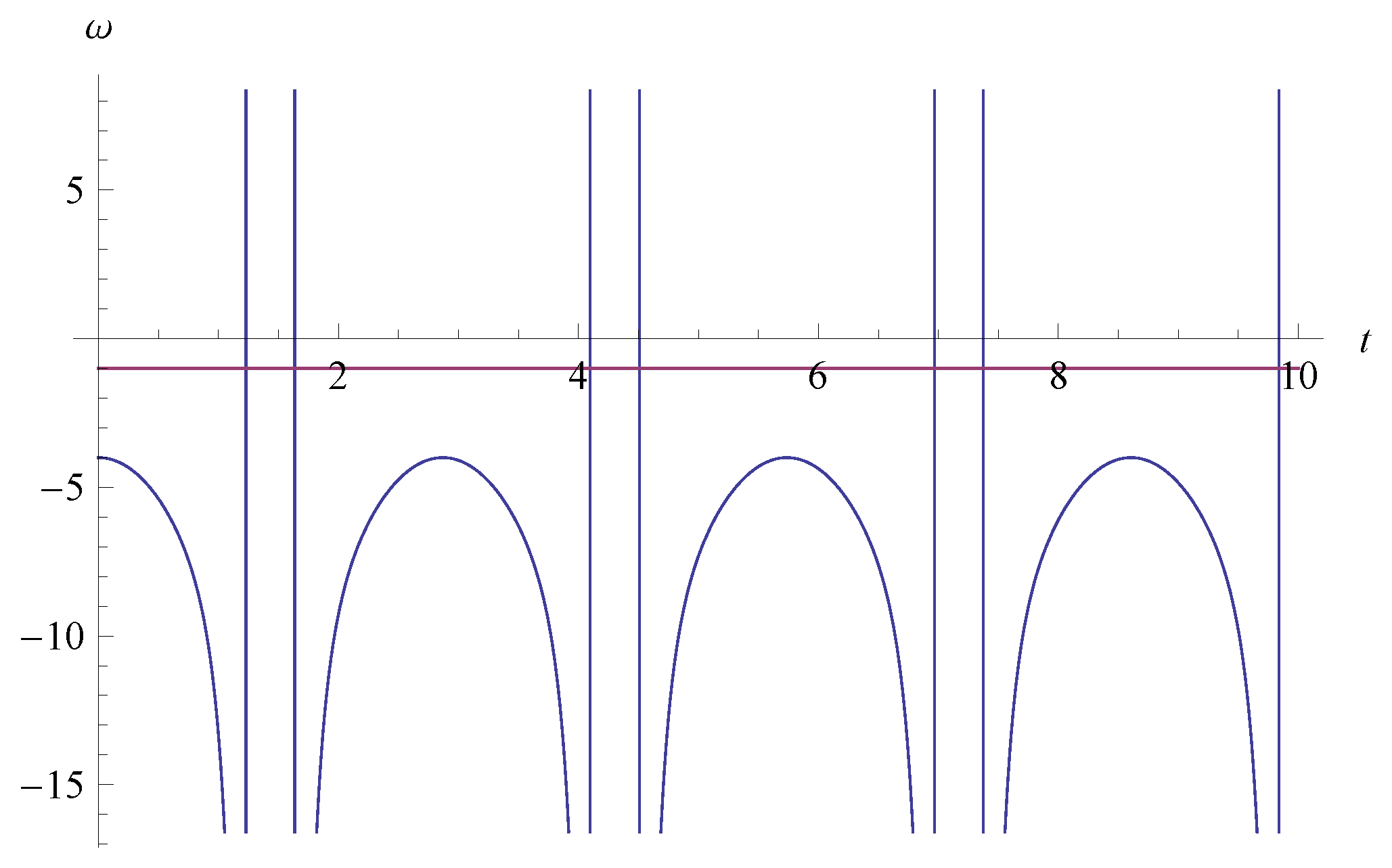
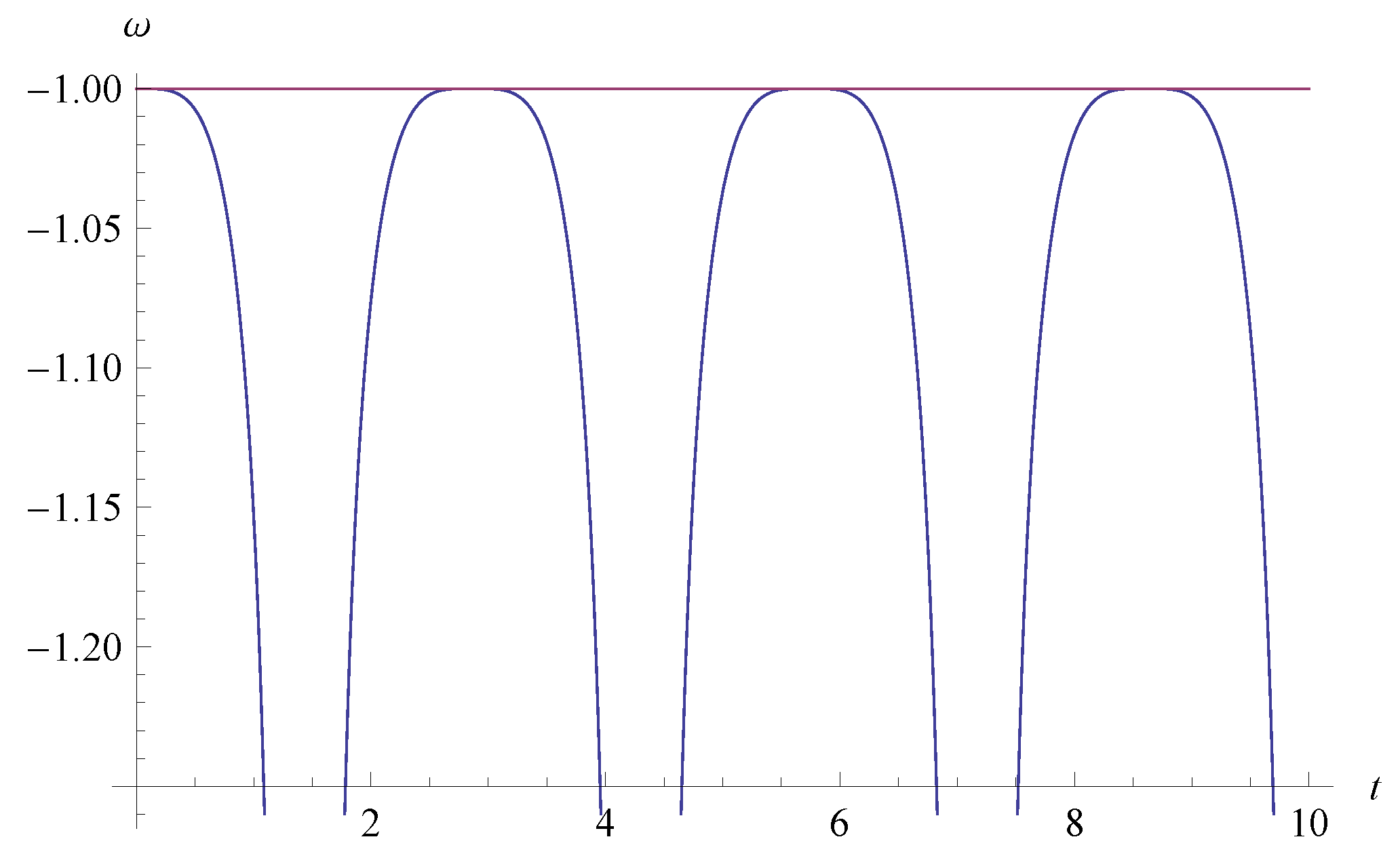
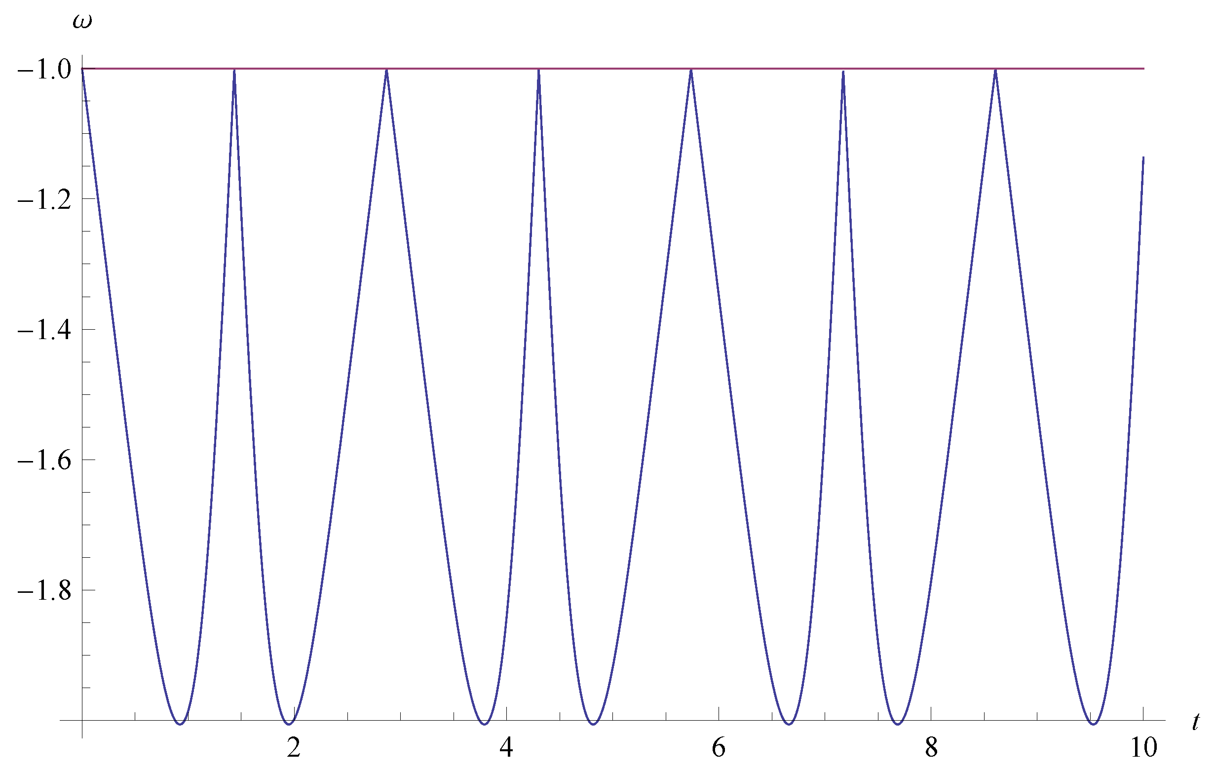
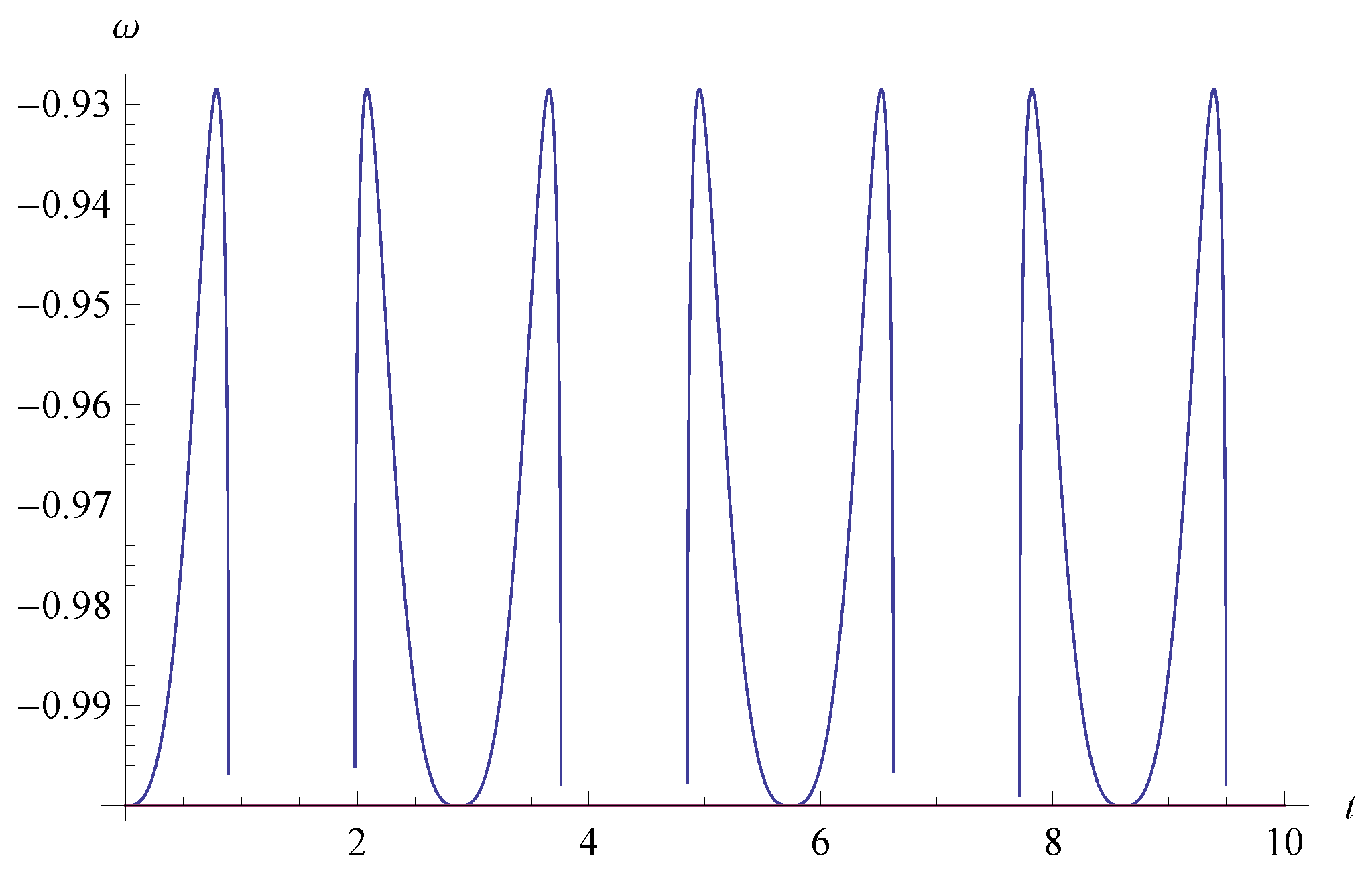
3.1. Periodical Generalizations
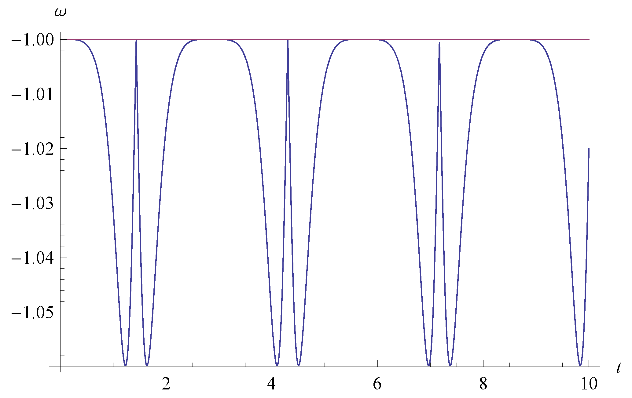
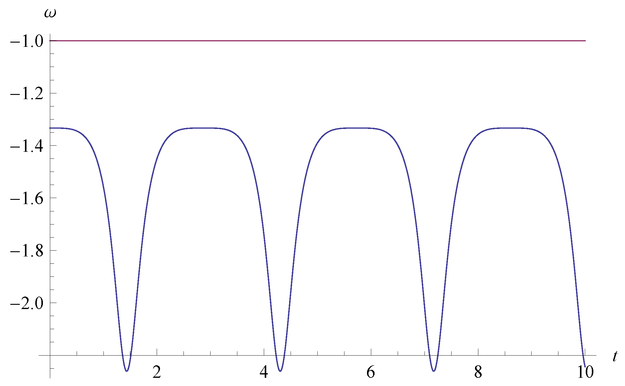
3.1.1. MG-XXI Model

One of the most interesting examples of gases is the MG-XXI model, which has the following EoS [103,104,105,106]:
p = B [ ( ρ ) ] 0.5
where B ( > 0 ) is a positive constant. By using the degenerate case of the function ( ρ ) in Equation (6), we can show that the well-known CG model [115] p = B / ρ , which is equal to Equation (4) with B = C 1 and α = 1 , is particular case of the MG-XXI model in Equation (7). The parameter of the EoS ω for our model is given by:
ω p ρ = B ( ρ ) ρ

3.1.2. MG-XXII Model

One of the two periodical generalizations of the GCG is given by [103,104,105,106]:
p = B [ ( ρ ) ] 0.5 α
In fact, its degenerate case is the GCG [116] p = B / ρ α , which is equivalent to Equation (3) with B = C 1 . For this model, the parameter of the EoS looks like:
ω = B [ ( ρ ) ] 0.5 α ρ

3.1.3. MG-XXIII Model

Next, we present one of the two periodical generalizations of the MCG. Its EoS reads [103,104,105,106]:
p = A ρ B [ ( ρ ) ] 0.5 α
where A is a constant. The corresponding parameter of the EoS is:
ω = A B [ ( ρ ) ] 0.5 α ρ

3.1.4. MG-XXIV Model

We now give a more general form of two periodical generalizations of the MCG. Its EoS is described as:
p = A [ ( ρ ) ] 0.5 B [ ( ρ ) ] 0.5 α
The parameter of the EoS for the model is written by:
ω = A [ ( ρ ) ] 0.5 ρ B [ ( ρ ) ] 0.5 α ρ
Again, by using the degenerate properties of the elliptic functions, we can demonstrate that this model is reduced to MCG.

3.2. Quasi-periodical Generalizations

In the preceding subsection, we have considered two periodical generalizations of CG type models. In this subsection, we study quasi-periodical models.

3.2.1. MG-XXV Model

One of the quasi-periodical models, the so-called MG-XXV model, is given by:
p = A σ ( ρ ) B [ σ ( ρ ) ] α
where A and B are constants and σ ( ρ ) is the Weierstrass σ-function. As the σ-function degenerates according to equations in (6), in this case Equation (15) becomes the MCG in Equation (5). The corresponding parameter of the EoS is expressed as:
ω = A σ ( ρ ) ρ B ρ [ σ ( ρ ) ] α

3.2.2. MG-XXVI Model

Our next quasi-periodical model is given by:
p = A ζ ( ρ ) B [ ζ ( ρ ) ] α
where ζ ( x ) is the Weierstrass ζ ( x ) -function. It is the MG-XXVI model. For the degenerate case in Equation (6), this model is also reduced to the MCG. Its parameter of the EoS takes the form:
ω = A ρ ζ ( ρ ) B [ ζ ( ρ ) ] α ρ

3.2.3. MG-XXVII Model

We explore the MG-XXVII model. For this model, the EoS reads:
p = A a m ( ρ ) B [ a m ( ρ ) ] α
where a m ( x ) is the Jacobi amplitude ( a m ( x ) ) function and α is a constant. In case of the degeneration in Equation (6), this model recovers the MCG. The parameter of the EoS is written by:
ω = A a m ( ρ ) ρ B [ a m ( ρ ) ] α ρ
It is significant to emphasize that (a) if we substitute σ ( t ) in Equation (6) into Equation (15); (b) if we use ζ ( t ) in Equation (6) and Equation (17); (c) if we combine ( t ) in Equation (6) with Equation (19), then we obtain the MCG in Equation (5). As a result, in the limit of m 1 = and m 2 = , the MG-XXV, MG-XXVI and MG-XXIV models are reduced to the MCG [117,119]. This point is the most important and novel observation in this work.
In the limit of the small energy density ρ 0 as well as ρ , the behaviors of the EoS for the universe in the MG-XXI, MG-XXIV, MG-XXV, MG-XXVI and MG-XXVII models asymptotically approach those in the CG model. On the other hand, in the middle regime of ρ, since the EoS for the universe in the MG-XXI, MG-XXIV, MG-XXV, MG-XXVI and MG-XXVII models is described by using elliptic functions with a periodic or quasi-periodic property, the EoS for the universe expresses also periodic or quasi-periodic behaviors.
From the above considerations, the cosmological evolution of the universe is described as follows. First, the energy responsible for inflation would be released to radiation (i.e., relativistic matter) through a reheating process and the universe enters the radiation dominated stage. Here, the concrete mechanism for both inflation and the reheating stage is not specified. After that, as the universe expands, its temperature decreases in proportion to a 1 , and the matter (i.e., non-relativistic matter) dominated stage appears. This can be seen in our models in the limit of ρ , namely ω asymptotically approaches zero, which corresponds to the EoS of the dust. Finally, the universe enters the dark energy dominated stage. This can also be understood in the limit of ρ 0 , where ω < 1 / 3 . Thus, it is considered that the cosmological evolution of the universe can be realized in our models.

4. Other Two Periodical FLRW Models

The EoS for dark energy is one of the most significant cosmological quantities. In this paper, we concentrate on the evolution of the EoS for dark energy. In the FLRW spacetime, the effective EoS for the universe is given by [19,20] ω eff p eff / ρ eff = 1 2 H ˙ / 3 H 2 . Here, ρ eff and p eff can be considered as the total energy density and pressure of the universe, respectively. Since we examine the dark energy dominated stage, the energy density ρ DE and pressure p DE of dark energy can be regarded as ρ DE ρ eff and p DE p eff . As a result, we find ω DE ω eff .
In addition, we represent ρ DE and p DE as ρ in Equation (2) and p in Equation (1), respectively. In the non-phantom (quintessence) phase, H ˙ < 0 and hence ω eff > 1 , which is the non-phantom (quintessence) phase, while in the phantom phase H ˙ > 0 and therefore ω eff < 1 . If H ˙ = 0 , ω eff = 1 , which is the case that dark energy is the cosmological constant.
As a qualitative criterion to constrain the models, we examine the evolution of the EoS ω of a fluid corresponding to dark energy. If ω is always less than 1 , the universe stays in the phantom phase in all the cosmic evolution history. This case is clearly inconsistent with the standard cosmological evolution and hence it can be ruled out. On the other hand, if ω is always larger than 1 or it crosses the line of 1 , these cases are not ruled out, namely these models may have the possibility to realize the standard evolution history of the universe.
In this section, we study two new periodical FLRW models. These models are expressed by using the Weierstrass ( t ) -function, which as well known satisfies the following ordinary differential equations [126]:
˙ 2 ( t ) = 4 3 ( t ) g 2 ( t ) g 3
¨ ( t ) = 6 2 ( t ) 0 . 5 g 2
( t ) = 12 ( t ) ˙ ( t )
( t ) = 120 3 ( t ) 18 g 2 ( t ) 12 g 3
where ˙ ( t ) = d ( t ) / d t and so on. In what follows, by using the reconstruction method in [19,20,71,113,114], and the Weierstrass ( t ) -function, for ten models (the MG-i models where i = XII, XIII, XIV, XV, XVI, XVII, XVIII, XIX, XX, XXXIII), we reconstruct the EoS for dark energy and explore its cosmological evolution in FLRW cosmology.

4.1. MG-XII Model

We suppose that the Hubble parameter is represented as:
H = ( t )
From this expression, the scale factor becomes:
a ( t ) = a 0 e ζ ( t )
where a 0 ( > 0 ) is a positive constant and ζ ( t ) is the Weierstrass ζ ( t ) -function. Then, Equation (25) and the gravitational field Equations (1) and (2) lead to the parametric EoS:
p = 2 4 3 ( t ) g 2 ( t ) g 3 3 2 ( t )
ρ = 3 2 ( t ) .
By using Equations (27) and (28), we see that the EoS parameter is written as:
ω = p ρ = 1 2 4 3 ( t ) g 2 ( t ) g 3 3 2 ( t )
In order to describe our models in terms of the scalar field theory, we introduce a scalar field ϕ and its self-interacting potential V ( ϕ ) . The Lagrangian for the scalar field theory is given by (see, e.g., [19,20]):
L ϕ = 0 . 5 ϕ ˙ 2 V ( ϕ )
Thus, this scalar is corresponding to a phantom one with ω < 1 , which can be seen in Equation (29). The energy momentum tensor of the scalar field ϕ ( t ) is identical to a fluid with the energy density ρ ϕ and pressure p ϕ given by:
ρ ϕ = 0.5 ϕ ˙ 2 + V ( ϕ ) = ρ
p ϕ = 0.5 ϕ ˙ 2 V ( ϕ ) = p
By using these expressions, we find:
ϕ ˙ 2 = ρ + p
V ( ϕ ) = 0.5 ( ρ p )
In addition, it follows from Equations (33) and (34) that the scalar field ϕ and self-interacting potential V ( ϕ ) are written as:
ϕ = i 2 4 3 ( t ) g 2 ( t ) g 3 d t
V = 3 2 t + 4 3 t g 2 t g 3
In Figure 1, we show the cosmological evolution of EoS ω as a function of t for t , 1 , 1 , i.e., the model parameters of the Weierstrass invariants of g 2 = 1 and g 3 = 1 . From Figure 1, we see that the universe always stays in the phantom phase ( ω < 1 ). Hence, this model is ruled out. Furthermore, we find the two periodic oscillatory behavior of ω.
Figure 1. The EoS ω in Equation (29) as a function of t for t , 1 , 1 , i.e., the model parameters of the Weierstrass invariants of g 2 = 1 and g 3 = 1 . The line of ω = 1 is also plotted.
Entropy 14 02351 g001
We remark a point in terms of the expression of V. In the above procedure, first the form of the scale factor a = a ( t ) or the Hubble parameter H = H ( t ) is supposed. Next, from this form we obtain the pressure p = p ( t ) and the energy density ρ = ρ ( t ) . On the other hand, in the description of the scalar field theory, the scalar field ϕ = ϕ ( t ) and its potential V = V ( ϕ ) are expressed with p = p ( t ) and ρ = ρ ( t ) . Accordingly, V = V ( ϕ ) = V ( ϕ ( t ) ) . This means that V is written as a function of cosmic time t. Thus, in principle, if a, H, p and ρ are inversely solved in terms of t, V can also be described by the expressions of a, H, p and ρ.

4.2. MG-XIII Model

We express the Hubble parameter as:
H = ˙ ( t )
From this expression, the scale factor is given by:
a ( t ) = a 0 e ( t )
By combining Equation (37) with the gravitational field Equations: (1) and (2), we find that the parametric EoS is written as:
p = 12 3 ( t ) 12 2 ( t ) + 3 g 2 ( t ) + g 2 + 3 g 3
ρ = 3 4 3 ( t ) g 2 ( t ) g 3
It follows from Equations (39) and (40) that the EoS parameter is given by:
ω = 12 3 ( t ) + 12 2 ( t ) 3 g 2 ( t ) g 2 3 g 3 3 4 3 ( t ) g 2 ( t ) g 3
By using Equations (33) and (34), we obtain the expressions of the scalar field ϕ and self-interacting potential V ( ϕ ) :
ϕ = 12 2 t + g 2 d t
V = 12 3 t + 6 2 t 3 g 2 t 3 g 3 0.5 g 2
In Figure 2, we depict the cosmological evolution of EoS ω as a function of t for t , 1 , 1 . From Figure 2, we see that the universe always evolves within the phantom phase ( ω < 1 ). Consequently, this model is ruled out.
Figure 2. The EoS ω in Equation (41) as a function of t. The legend is the same as in Figure 1.
Entropy 14 02351 g002

4.3. MG-XIV Model

We provide that the Hubble parameter is described as:
H = ¨ ( t )
so that the scale factor can read as:
a ( t ) = a 0 e ˙ ( t )
From Equation (44) and the gravitational field Equations (1) and (2), we have the parametric EoS:
p = 24 ( t ) 4 3 ( t ) g 2 ( t ) g 3 3 6 2 ( t ) 0.5 g 2 2
ρ = 3 6 2 ( t ) 0.5 g 2 2
Hence, the EoS parameter is written as:
ω = 1 8 ( t ) 4 3 ( t ) g 2 ( t ) g 3 6 2 ( t ) 0.5 g 2 2
With Equations (33) and (34), we have:
ϕ = 2 i 6 t 4 3 t g 2 t g 3 d t
V ϕ = 3 6 2 t 0.5 g 2 2 + 12 t 4 3 t g 2 t g 3
In Figure 3, we illustrate the cosmological evolution of EoS ω as a function of t for t , 1 , 1 . From Figure 3, we see that the universe always stays in the non-phantom (quintessence) phase ( ω > 1 ).
Figure 3. The EoS ω in Equation (48) as a function of t. The legend is the same as in Figure 1.
Entropy 14 02351 g003

4.4. MG-XV Model

We take the form of the Hubble parameter as:
H = ( t )
From this form, the corresponding scale factor is given by:
a ( t ) = a 0 e ¨ ( t )
With Equation (51) and the gravitational field Equations (33) and (34), we obtain the parametric EoS:
p = 12 20 3 ( t ) 3 g 2 ( t ) 2 g 3 432 2 ( t ) 4 3 ( t ) g 2 ( t ) g 3
ρ = 432 ( t ) 2 4 3 ( t ) g 2 ( t ) g 3
It follows from Equations (53) and (54) that the parametric EoS is given by:
ω = 1 20 3 ( t ) 3 g 2 ( t ) 2 g 3 36 ( t ) 2 4 3 ( t ) g 2 ( t ) g 3
By using the formulae in Equations (33) and (34), we acquire:
ϕ = 2 i 3 20 3 t 3 g 2 t 2 g 3 d t
V ϕ = 6 20 3 ( t ) 3 g 2 ( t ) 2 g 3 + 432 2 t 4 3 t g 2 t g 3
In Figure 4, we display the cosmological evolution of EoS ω as a function of t for t , 1 , 1 . From Figure 4, we understand that the universe always evolves within the phantom phase ( ω < 1 ). Thus, this model is ruled out.
Figure 4. The EoS ω in Equation (55) as a function of t. The legend is the same as in Figure 1.
Entropy 14 02351 g004

4.5. MG-XVI Model

We assume that the Hubble parameter is written as:
H = ( t )
In this case, the scale factor becomes:
a ( t ) = a 0 e ( t )
Using Equation (58) and the gravitational field Equations: (1) and (2) yields:
p = 36 20 2 ( t ) g 2 4 3 ( t ) g 2 ( t ) g 3 3 120 3 ( t ) 18 g 2 ( t ) 12 g 3 2
ρ = 3 120 3 ( t ) 18 g 2 ( t ) 12 g 3 2
Hence, the parametric EoS is expressed as:
ω = 1 12 20 2 ( t ) g 2 4 3 ( t ) g 2 ( t ) g 3 120 3 ( t ) 18 g 2 ( t ) 12 g 3 2
From Equations (33) and (34), we acquire:
ϕ = 6 i 20 2 ( t ) g 2 4 3 t g 2 t g 2 d t
V = 18 20 2 ( t ) g 2 4 3 t g 2 t g 2 + 3 120 3 t 18 g 2 t 12 g 3 2
In Figure 5, we plot the cosmological evolution of EoS ω as a function of t for t , 1 , 1 . From Figure 5, we find that the universe always evolves within the phantom phase ( ω < 1 ). Therefore, this model is ruled out. In addition, we clearly see the two periodic oscillating evolution of ω.
Figure 5. The EoS ω in Equation (62) as a function of t. The legend is the same as in Figure 1.
Entropy 14 02351 g005

4.6. MG-XVII Model

We take the scale factor as:
a t = ( t )
From this expression, the Hubble parameter becomes:
H = 4 3 t g 2 t g 3 t
Equation (66) and the gravitational field Equations (1) and (2) present the parametric EoS:
p = 16 3 t 2 g 2 t g 3 2 t
ρ = 3 4 3 t g 2 t 3 g 3 2 t
Furthermore, the EoS parameter is represented as:
ω = 16 3 t 2 g 2 t g 3 12 3 t 3 g 2 t 3 g 3
From Equations (33) and (34), we have:
ϕ = i 4 3 t + g 2 t + 2 g 3 t d t
V = 28 2 t 5 g 2 t 4 g 3 2 2 t
In Figure 6, we plot the cosmological evolution of EoS ω as a function of t for t , 1 , 1 . From Figure 6, we see that the universe always stays in the phantom phase ( ω < 1 ). Accordingly, this model is ruled out.
Figure 6. The EoS ω in Equation (69) as a function of t. The legend is the same as in Figure 1.
Entropy 14 02351 g006

4.7. MG-XVIII Model

We describe the scale factor as:
a = ˙ ( t )
It follows from this description that the Hubble parameter is given by:
H = 6 2 t 0 . 5 g 2 4 3 t g 2 t g 3

4.8. MG-XIX Model

We consider that the scale factor is given by:
a = ¨ ( t )
so that the Hubble parameter can read:
H = 12 t 4 3 t g 2 t g 3 6 2 t 0 . 5 g 2

4.9. MG-XX Model

We suppose the following form of the scale factor:
a = ( t )
From this representation, the Hubble parameter is written by:
H = 20 3 t 3 g 2 t 2 g 3 2 t 4 3 t g 2 t g 3

4.10. MG-XXXIII Model

We suppose that the scale factor takes the following form:
a = ( t )
It follows from this representation that the Hubble parameter is described by:
H = 3 ( g 2 20 2 t ) ( g 3 + g 2 2 t 4 3 t ) 2 g 3 + 3 g 2 t 20 3 t
It is important to mention that a quintom model (where there must exist both canonical and non-canonical scalar fields in order that the crossing of the phantom divide can occur) with single canonical scalar field cannot be reconstructed, in which the crossing of the phantom divide cannot occur [127]. As explained in the MG-XVIII, XIX, XX and XXXIII models (in Section 4.7, Section 4.8, Section 4.9 and Section 4.10, respectively), if we reconstruct the corresponding single scalar field model, the crossing of the phantom divide can be realized. Thus, this implies that for these models, such a reconstruction is not physical but just a mathematical procedure.
The physical interpretation of our results is considered as follows. By reconstructing the expansion behavior of the universe, i.e., the Hubble parameter, with the Weierstrass ( t ) -function, which has a periodic property, the periodic behavior of the EoS for the universe can be realized. Such a procedure can be applied to scenarios to avoid cosmological singularities and eventually a non-singular universe can be realized.
It is also remarkable to note that in terms of all the numerical calculations in Figure 1, Figure 2, Figure 3, Figure 4, Figure 5 and Figure 6, the qualitative results do not strongly depend on the initial conditions and the model parameters such as the Weierstrass ( t ) -function.
Moreover, for all the models, the scale factor a has to be positive and the Hubble parameter H should be real. From Equations (26), (38), (45), (52) and (59), a is always positive. Also, it follows from Equations (65), (72), (74), (76) and (78) that a is written by ( t ) or its time derivatives. By using the Laurent expansion of ( t ) around t = 0 as ( t ) = 1 / t 2 + g 2 / 20 t 2 + g 3 / 28 t 4 + O ( t 6 ) , we find ˙ ( t ) = 2 / t 3 + g 2 / 10 t + g 3 / 7 t 3 + O ( t 5 ) , ¨ ( t ) = 6 / t 4 + g 2 / 10 + 3 g 3 / 7 t 2 + O ( t 4 ) , ( t ) = 24 / t 5 + 6 g 3 / 7 t + O ( t 3 ) , and ( t ) = 120 / t 5 + 6 g 3 / 7 + O ( t 2 ) . Thus, for the cases of a = ˙ ( t ) in Equation (72) and a = ( t ) in Equation (76), around t = 0 , the expression of a is not well defined because the value of a would become negative around t = 0 . In this sense, around t = 0 , the MG-XVIII and MG-XX models cannot be used. On the other hand, since the argument of the Weierstrass functions used in this paper is the cosmic time t, which is real, all the values of the Weierstrass functions are real. In all the models, H is described by the Weierstrass functions and hence H would be real.
Furthermore, we state that if the evolution of ω is displayed as a function of the red shift z a p / a 1 with a p the present value of a, the direction of the cosmic time t to go by becomes opposite to that for ω to be shown as a function of t in Figure 1, Figure 2, Figure 3, Figure 4, Figure 5 and Figure 6. It would be considered that the main qualitative difference is only this point and hence other cosmological consequences do not change.
In addition, it is interesting to note that the models examined in this work may solve not only the dark energy paradigm but also the horizon and flatness problems. In other words, these models may produce a kind of inflationary epoch or perhaps a contraction phase as in the ekpyrotic scenario. In order for inflation or the ekpyrotic scenario to be realized realistically, it is necessary to consider the way of connecting the inflationary stage and the dark energy dominated stage, i.e., the realization of the reheating stage. This is a crucial point for these models to be realistic inflation models or the ekpyrotic scenario.
Moreover, it should be cautioned that in Figure 2, Figure 3 and Figure 4, apparently the EoS ω diverges. However, the reason is just a way of plotting and therefore there is no divergence in terms of the EoS in all of the figures.
Finally, we mention the issue of existence of a ghost, namely, the instability for the case of the crossing of the phantom divide. For a scalar field theory, it is known that if the crossing of the phantom divide happens in the FLRW universe, there would appear a ghost. In Section 4, we have presented the interpretations of our models in the framework of a scalar field theory. However, there still exists the possibility that our models could be regarded as a more complicated theory, e.g., which is described by the non-linear kinetic terms such as k-essence models [128,129,130,131,132,133] and the Galileon models [134,135,136,137,138]. These investigations might be one of the interesting future works in our approach to the periodic and quasi-periodic generalizations of the Chaplygin gas type models.

5. Conclusions

In the present paper, we have reconstructed periodic and quasi-periodic generalizations of the Chaplygin gas type models by using the Weierstrass ( t ) , σ ( t ) and ζ ( t ) -elliptic functions. We have explored the cosmological evolution of the EoS for dark energy in FLRW spacetime. In particular, we have shown that by using the degenerate properties of the elliptic functions, the MCG models can be recovered. This is one of the most important cosmological ingredients obtained in this paper. This result implies that by plugging the reconstruction method of the expansion history of the universe with the Weierstrass elliptic functions, we can acquire the MCG models, which have a potential to reveal the properties of both dark energy and dark matter. In other words, the procedure demonstrated in this paper can lead to a preferable cosmological model by starting with the mathematical special functions.
It is meaningful to summarize the following significant points. (a) The Weierstrass functions have two periods m 1 and m 2 . This is their essential property. (b) Our periodic and quasi-periodic models given in Section 3 are periodic or quasi-periodic in terms of the energy density ρ. (c) Furthermore, if the special values of the periods m 1 and m 2 are infinite, these models in Section 3 are transformed into or have limits of the Chaplygin gas models, which can be seen from the formulae in Section 3.1. Thus, in this sense to reconstruct these models is considered as two periodic or quasi-periodical generalizations of the CG models. This is the justification of application of the Weierstrass functions to cosmological models. (d) Our models presented in Section 4 are periodic on the cosmic time t (which is here dimensionless), in contrast to the models in Section 3, which are periodic/quasi-periodic on ρ. (e) Moreover, our periodic/quasi-periodic models in Section 3 are singular at ρ = 0 and those in Section 4 at t = 0 .
It is also important to emphasize that the cosmological advantage to acquire the periodic evolution of the universe is to realize scenarios to avoid a Big Bang singularity, the finite-time future singularities and a Big Crunch singularity. By applying the obtained results and the discussed procedure to scenarios for the avoidance of singularities, e.g., the cyclic universe, the ekpyrotic scenario and the bouncing universe, we can find a non-singular cosmology.
Furthermore, it has explicitly been illustrated that there are three type models with realizing the cosmological evolution of the EoS for dark energy: (i) the universe always stays in the non-phantom (quintessence) phase (the MG-XIV model); (ii) the universe always evolves within the phantom phase (the MG-XII, MG-XIII, MG-XV, MG-XVI and MG-XVII models); (iii) the crossing of the phantom divide can be realized (the MG-XVIII, MG-XIX, MG-XX and MG-XXXIII models). If the universe always stays in the phantom phase, it is impossible to describe the whole evolution history of the universe, i.e., the decelerated phases such as the radiation and matter dominated stages. Thus, these models are ruled out. In addition, the corresponding description of a canonical scalar field model to the models in the above (iii) category is not physical but just mathematical, because in the light of quintom model [127], it is impossible for a single canonical scalar field to realize the crossing of the phantom divide.
The scalar fields and the corresponding potentials have been analyzed for different types of MG models mentioned above. The EoS parameters have been derived and their natures have also been illustrated graphically during the evolution of the universe.
On the other hand, at the current stage the cosmological constant is consistent with the observational data [4], but there still exists the possibility of dynamical dark energy, which is, e.g., described by a scalar field or a fluid. Thus, when we acquire the results of data analysis of the more precise future experiments like by the PLANCK satellite [139], it is strongly expected that the investigations on the phase of the universe (i.e., the non-phantom or phantom phase) or the crossing of the phantom divide can become more meaningful. In the future work, it would be interesting to test whether the above models may be suitable candidates for dark energy by coming observational data fittings.

Acknowledgments

K.B. would like to sincerely acknowledge very kind and warm hospitality at Eurasian National University very much, where this work has been completed.

References

  1. Spergel, D.N.; Verde, L.; Peiris, H.V.; Komatsu, E.; Nolta, M.R.; Bennett, C.L.; Halpern, M.; Hinshaw, G.; Jarosik, N.; Kogut, A.; et al. First Year Wilkinson Microwave Anisotropy Probe (WMAP) Observations: Determination of Cosmological Parameters. Astrophys. J. Suppl. 2003, 148, 175–194. [Google Scholar] [CrossRef]
  2. Spergel, D.N.; Bean, R.; Dore, O.; Nolta, M.R.; Bennett, C.L.; Hinshaw, G.; Jarosik, N.; Komatsu, E.; Page, L.; Peiris, H.V.; et al. Wilkinson Microwave Anisotropy Probe (WMAP) three year results: Implications for cosmology. Astrophys. J. Suppl. 2007, 170, 377–408. [Google Scholar] [CrossRef]
  3. Komatsu, E.; Dunkley, J.; Nolta, M.R.; Bennett, C.L.; Gold, B.; Hinshaw, G.; Jarosik, N.; Larson, D.; Limon, M.; Page, L.; et al. Five-Year Wilkinson Microwave Anisotropy Probe (WMAP) Observations: Cosmological Interpretation. Astrophys. J. Suppl. 2009, 180, 330–376. [Google Scholar] [CrossRef]
  4. Komatsu, E.; Smith, K.M.; Dunkley, J.; Bennett, C.L.; Gold, B.; Hinshaw, G.; Jarosik, N.; Larson, D.; Nolta, M.R.; Page, L.; et al. Seven-Year Wilkinson Microwave Anisotropy Probe (WMAP) Observations: Cosmological Interpretation. Astrophys. J. Suppl. 2011, 192, 18. [Google Scholar] [CrossRef]
  5. Perlmutter, S.; Aldering, G.; Goldhaber, G.; Knop, R.A.; Nugent, P.; Castro, P.G.; Deustua, S.; Fabbro, S.; Goobar, A.; Groom, D.E.; et al. Measurements of Omega and Lambda from 42 High-Redshift Supernovae. Astrophys. J. 1999, 517, 565–586. [Google Scholar] [CrossRef]
  6. Riess, A.G.; Filippenko, A.V.; Challis, P.; Clocchiattia, A.; Diercks, A.; Garnavich, P.M.; Gilliland, R.L.; Hogan, C.J.; Jha, S.; Kirshner, R.P.; et al. Observational Evidence from Supernovae for an Accelerating Universe and a Cosmological Constant. Astron. J. 1998, 116, 1009–1038. [Google Scholar] [CrossRef]
  7. Tegmark, M.; Strauss, M.A.; Blanton, M.R.; Abazajian, K.N.; Dodelson, S.; Sandvik, H.; Wang, X.; Weinberg, D.H.; Zehavi, I.; Bahcall, N.A.; et al. Cosmological parameters from SDSS and WMAP. Phys. Rev. D 2004. [Google Scholar] [CrossRef]
  8. Seljak, U.; Makarov, A.; McDonald, P.; Anderson, S.; Bahcall, N.; Brinkmann, J.; Burles, S.; Cen, R.; Doi, M.; Gunn, J.; Ivezic, Z.; et al. Cosmological parameter analysis including SDSS Ly-alpha forest and galaxy bias: Constraints on the primordial spectrum of fluctuations, neutrino mass, and dark energy. Phys. Rev. D 2005. [Google Scholar] [CrossRef]
  9. Eisenstein, D.J.; Zehavi, I.; Hogg, D.W.; Scoccimarro, R.; Blanton, M.R.; Nichol, R.C.; Scranton, R.; Seo, H.; Tegmark, M.; Zheng, Z.; et al. Detection of the Baryon Acoustic Peak in the Large-Scale Correlation Function of SDSS Luminous Red Galaxies. Astrophys. J. 2005, 633, 560–574. [Google Scholar] [CrossRef]
  10. Jain, B.; Taylor, A. Cross-correlation Tomography: Measuring Dark Energy Evolution with Weak Lensing. Phys. Rev. Lett. 2003, 91, 141302. [Google Scholar] [CrossRef] [PubMed]
  11. Copeland, E.J.; Sami, M.; Tsujikawa, S. Dynamics of dark energy. Int. J. Mod. Phys. D 2006, 15, 1753–1936. [Google Scholar] [CrossRef]
  12. Durrer, R.; Maartens, R. Dark Energy and Dark Gravity. Gen. Rel. Grav. 2008, 40, 301–328. [Google Scholar] [CrossRef] [Green Version]
  13. Durrer, R.; Maartens, R. Dark Energy and Modified Gravity. In Dark Energy: Observational Theoretical Approaches; Ruiz-Lapuente, P., Ed.; Cambridge University press: Cambridge, UK, 2010; pp. 48–91. [Google Scholar]
  14. Cai, Y.F.; Saridakis, E.N.; Setare, M.R.; Xia, J.Q. Quintom Cosmology: Theoretical implications and observations. Phys. Rept. 2010, 493, 1–60. [Google Scholar] [CrossRef]
  15. Tsujikawa, S. Dark energy: investigation and modeling. 2010; arXiv:1004.1493 [astro-ph.CO]. [Google Scholar]
  16. Amendola, L.; Tsujikawa, S. Dark Energy; Cambridge University press: Cambridge, United Kingdom, 2010; pp. 1–491. [Google Scholar]
  17. Li, M.; Li, X.D.; Wang, S.; Wang, Y. Dark Energy. Commun. Theor. Phys. 2011, 56, 525–604. [Google Scholar] [CrossRef]
  18. Bamba, K.; Capozziello, S.; Nojiri, S.; Odintsov, S.D. Dark energy cosmology: the equivalent description via different theoretical models and cosmography tests. Astrophys. Space Sci. 2012, 342, 155–228. [Google Scholar] [CrossRef]
  19. Nojiri, S.; Odintsov, S.D. Unified cosmic history in modified gravity: from F(R) theory to Lorentz non-invariant models. Phys. Rept. 2011, 505, 59–144. [Google Scholar] [CrossRef]
  20. Nojiri, S.; Odintsov, S.D. Introduction to modified gravity and gravitational alternative for dark energy. Int. J. Geom. Meth. Mod. Phys. 2007, 4, 115–146. [Google Scholar] [CrossRef]
  21. Sotiriou, T.P.; Faraoni, V. f(R) Theories Of Gravity. Rev. Mod. Phys. 2010, 82, 451–497. [Google Scholar] [CrossRef]
  22. Capozziello, S.; Faraoni, V. Beyond Einstein Gravity; Springer: London, UK, 2010; pp. 1–424. [Google Scholar]
  23. Capozziello, S.; de Laurentis, M. Extended Theories of Gravity. Phys. Rept. 2011, 509, 167–321. [Google Scholar] [CrossRef]
  24. De Felice, A.; Tsujikawa, S. f(R) theories. Living Rev. Rel. 2010, 13, 3. [Google Scholar] [CrossRef]
  25. Clifton, T.; Ferreira, P.G.; Padilla, A.; Skordis, C. Modified Gravity and Cosmology. Phys. Rept. 2012, 513, 1–189. [Google Scholar] [CrossRef]
  26. Capozziello, S.; de Laurentis, M.; Odintsov, S.D. Hamiltonian dynamics and Noether symmetries in Extended Gravity Cosmology. Eur. Phys. J. C 2012, 72, 2068. [Google Scholar] [CrossRef]
  27. Caldwell, R.R.; Kamionkowski, M.; Weinberg, N.N. Phantom Energy and Cosmic Doomsday. Phys. Rev. Lett. 2003. [Google Scholar] [CrossRef]
  28. McInnes, B. The dS/CFT correspondence and the big smash. J. High Energy Phys. 2002, 0208, 029. [Google Scholar] [CrossRef]
  29. Nojiri, S.; Odintsov, S.D. Quantum deSitter cosmology and phantom matter. Phys. Lett. B 2003, 562, 147–152. [Google Scholar] [CrossRef]
  30. Nojiri, S.; Odintsov, S.D. Effective equation of state and energy conditions in phantom / tachyon inflationary cosmology perturbed by quantum effects. Phys. Lett. B 2003, 571, 1–10. [Google Scholar] [CrossRef]
  31. Faraoni, V. Superquintessence. Int. J. Mod. Phys. D 2002, 11, 471–482. [Google Scholar] [CrossRef]
  32. Gonzalez-Diaz, P.F. K-essential phantom energy: Doomsday around the corner? Phys. Lett. B 2004, 586, 1–4. [Google Scholar] [CrossRef]
  33. Elizalde, E.; Nojiri, S.; Odintsov, S.D. Late-time cosmology in (phantom) scalar-tensor theory: Dark energy and the cosmic speed-up. Phys. Rev. D 2004. [Google Scholar] [CrossRef]
  34. Singh, P.; Sami, M.; Dadhich, N. Cosmological dynamics of phantom field. Phys. Rev. D 2003. [Google Scholar] [CrossRef]
  35. Csaki, C.; Kaloper, N.; Terning, J. Exorcising w < −1. Annals Phys. 2005, 317, 410–422. [Google Scholar]
  36. Wu, P.X.; Yu, H.W. Avoidance of Big Rip In Phantom Cosmology by Gravitational Back Reaction. Nucl. Phys. B 2005, 727, 355–367. [Google Scholar] [CrossRef]
  37. Nesseris, S.; Perivolaropoulos, L. The fate of bound systems in phantom and quintessence cosmologies. Phys. Rev. D 2004. [Google Scholar] [CrossRef]
  38. Sami, M.; Toporensky, A. Phantom Field and the Fate of Universe. Mod. Phys. Lett. A 2004, 19, 1509–1517. [Google Scholar] [CrossRef]
  39. Stefancic, H. Generalized phantom energy. Phys. Lett. B 2004, 586, 5–10. [Google Scholar] [CrossRef]
  40. Chimento, L.P.; Lazkoz, R. On the link between phantom and standard cosmologies. Phys. Rev. Lett. 2003. [Google Scholar] [CrossRef]
  41. Hao, J.G.; Li, X.Z. Generalized quartessence cosmic dynamics: Phantom or quintessence with de Sitter attractor. Phys. Lett. B 2005, 606, 7–11. [Google Scholar] [CrossRef]
  42. Elizalde, E.; Nojiri, S.; Odintsov, S. D.; Wang, P. Dark energy: Vacuum fluctuations, the effective phantom phase, and holography. Phys. Rev. D 2005. [Google Scholar] [CrossRef]
  43. Dabrowski, M.P.; Stachowiak, T. Phantom Friedmann cosmologies and higher-order characteristics of expansion. Annals Phys. 2006, 321, 771–812. [Google Scholar] [CrossRef]
  44. Lobo, F.S.N. Phantom energy traversable wormholes. Phys. Rev. D 2005. [Google Scholar] [CrossRef]
  45. Cai, R.G.; Zhang, H.S.; Wang, A. Crossing w = -1 in Gauss-Bonnet brane world with induced gravity. Commun. Theor. Phys. 2005, 44, 948–954. [Google Scholar] [CrossRef]
  46. Aref’eva, I.Y.; Koshelev, A.S.; Vernov, S.Y. Crossing of the w=-1 Barrier by D3-brane Dark Energy Model. Phys. Rev. D 2005. [Google Scholar] [CrossRef]
  47. Lu, H. Q.; Huang, Z.G.; Fang, W. Quantum and classical cosmology with Born-Infeld scalar field. 2005. [Google Scholar]
  48. Godlowski, W.; Szydlowski, M. Which cosmological model with dark energy - phantom or LambdaCDM. Phys. Lett. B 2005, 623, 10–16. [Google Scholar] [CrossRef]
  49. Sola, J.; Stefancic, H. Effective equation of state for dark energy: mimicking quintessence and phantom energy through a variable Lambda. Phys. Lett. B 2005, 624, 147–157. [Google Scholar] [CrossRef]
  50. Guberina, B.; Horvat, R.; Nikolic, H. Generalized holographic dark energy and the IR cutoff problem. Phys. Rev. D 2005. [Google Scholar] [CrossRef]
  51. Shtanov, Y.; Sahni, V. Unusual cosmological singularities in braneworld models. Class. Quant. Grav. 2002, 19, L101–L107. [Google Scholar] [CrossRef]
  52. Barrow, J.D. Sudden Future Singularities. Class. Quant. Grav. 2004, 21, L79–L82. [Google Scholar] [CrossRef]
  53. Nojiri, S.; Odintsov, S.D. Quantum escape of sudden future singularity. Phys. Lett. B 2004, 595, 1–8. [Google Scholar] [CrossRef]
  54. Nojiri, S.; Odintsov, S.D. The final state and thermodynamics of dark energy universe. Phys. Rev. D 2004. [Google Scholar] [CrossRef]
  55. Nojiri, S.; Odintsov, S.D. Inhomogeneous equation of state of the universe: Phantom era, future singularity and crossing the phantom barrier. Phys. Rev. D 2005. [Google Scholar] [CrossRef]
  56. Cotsakis, S.; Klaoudatou, I. Future singularities of isotropic cosmologies. J. Geom. Phys. 2005, 55, 306–315. [Google Scholar] [CrossRef]
  57. Dabrowski, M.P. Inhomogenized sudden future singularities. Phys. Rev. D 2005. [Google Scholar] [CrossRef]
  58. Fernandez-Jambrina, L.; Lazkoz, R. Geodesic behaviour of sudden future singularities. Phys. Rev. D 2004. [Google Scholar] [CrossRef]
  59. Fernandez-Jambrina, L.; Lazkoz, R. Singular fate of the universe in modified theories of gravity. Phys. Lett. B 2009, 670, 254–258. [Google Scholar] [CrossRef]
  60. Barrow, J.D.; Tsagas, C.G. New Isotropic and Anisotropic Sudden Singularities. Class. Quant. Grav. 2005, 22, 1563–1571. [Google Scholar] [CrossRef]
  61. Stefancic, H. ’Expansion’ around the vacuum equation of state: Sudden future singularities and asymptotic behavior. Phys. Rev. D 2005. [Google Scholar] [CrossRef]
  62. Cattoen, C.; Visser, M. Necessary and sufficient conditions for big bangs, bounces, crunches, rips, sudden singularities, and extremality events. Class. Quant. Grav. 2005, 22, 4913–4930. [Google Scholar] [CrossRef]
  63. Tretyakov, P.; Toporensky, A.; Shtanov, Y.; Sahni, V. Quantum effects, soft singularities and the fate of the universe in a braneworld cosmology. Class. Quant. Grav. 2006, 23, 3259–3274. [Google Scholar] [CrossRef]
  64. Balcerzak, A.; Dabrowski, M.P. Strings at future singularities. Phys. Rev. D 2006. [Google Scholar] [CrossRef]
  65. Sami, M.; Singh, P.; Tsujikawa, S. Avoidance of future singularities in loop quantum cosmology. Phys. Rev. D 2006. [Google Scholar] [CrossRef]
  66. Bouhmadi-Lopez, M.; Gonzalez-Diaz, P.F.; Martin-Moruno, P. Worse than a big rip? Phys. Lett. B 2008, 659, 1–5. [Google Scholar] [CrossRef]
  67. Yurov, A.V.; Astashenok, A.V.; Gonzalez-Diaz, P.F. Astronomical bounds on future big freeze singularity. Grav. Cosmol. 2008, 14, 205–212. [Google Scholar] [CrossRef]
  68. Koivisto, T. Dynamics of Nonlocal Cosmology. Phys. Rev. D 2008. [Google Scholar] [CrossRef]
  69. Barrow, J.D.; Lip, S.Z.W. The Classical Stability of Sudden and Big Rip Singularities. Phys. Rev. D 2009. [Google Scholar] [CrossRef]
  70. Bouhmadi-Lopez, M.; Tavakoli, Y.; Moniz, P.V. Appeasing the Phantom Menace? JCAP 2010, 1004, 016. [Google Scholar] [CrossRef]
  71. Nojiri, S.; Odintsov, S.D.; Tsujikawa, S. Properties of singularities in (phantom) dark energy universe. Phys. Rev. D 2005. [Google Scholar] [CrossRef]
  72. Nojiri, S.; Odintsov, S.D. The future evolution and finite-time singularities in F(R)-gravity unifying the inflation and cosmic acceleration. Phys. Rev. D 2008. [Google Scholar] [CrossRef]
  73. Bamba, K.; Nojiri, S.; Odintsov, S.D. The Universe future in modified gravity theories: Approaching the finite-time future singularity. JCAP 2008, 0810, 045. [Google Scholar] [CrossRef]
  74. Bamba, K.; Odintsov, S.D.; Sebastiani, L.; Zerbini, S. Finite-time future singularities in modified Gauss-Bonnet and F(R,G) gravity and singularity avoidance. Eur. Phys. J. C 2010, 67, 295–310. [Google Scholar] [CrossRef]
  75. Steinhardt, P.J.; Turok, N. Cosmic evolution in a cyclic universe. Phys. Rev. D 2002. [Google Scholar] [CrossRef]
  76. Steinhardt, P.J.; Turok, N. A cyclic model of the universe. Science 2002, 296, 1436–1439. [Google Scholar] [CrossRef] [PubMed]
  77. Khoury, J.; Ovrut, B.A.; Steinhardt, P.J.; Turok, N. Density perturbations in the ekpyrotic scenario. Phys. Rev. D 2002. [Google Scholar] [CrossRef]
  78. Steinhardt, P.J.; Turok, N. The cyclic universe: An informal introduction. Nucl. Phys. Proc. Suppl. 2003, 124, 38–49. [Google Scholar] [CrossRef]
  79. Steinhardt, P.J.; Turok, N. A cyclic model of the universe. Science 2002, 296, 1436–1439. [Google Scholar] [CrossRef] [PubMed]
  80. Khoury, J.; Steinhardt, P.J.; Turok, N. Designing Cyclic Universe Models. Phys. Rev. Lett. 2004. [Google Scholar] [CrossRef]
  81. Steinhardt, P.J.; Turok, N. Why the cosmological constant is small and positive. Science 2006, 312, 1180–1182. [Google Scholar] [CrossRef] [PubMed]
  82. Saaidi, K.; Sheikhahmadi, H.; Mohammadi, A.H. Interacting New Agegraphic Dark Energy in a Cyclic Universe. Astrophys. Space Sci. 2012, 338, 355–361. [Google Scholar] [CrossRef]
  83. Nojiri, S.; Odintsov, S.D.; Saez-Gomez, D. Cyclic, ekpyrotic and little rip universe in modified gravity. AIP Conf. Proc. 2011, 1458, 207–221. [Google Scholar]
  84. Cai, Y.F.; Saridakis, E.N. Non-singular Cyclic Cosmology without Phantom Menace. J. Cosmol. 2011, 17, 7238–7254. [Google Scholar]
  85. Sahni, V.; Toporensky, A. Cosmological Hysteresis and the Cyclic Universe. Phys. Rev. D 2012. [Google Scholar] [CrossRef]
  86. Chung, D.Y. The Cyclic universe. 2001; arXiv:physics/0105064. [Google Scholar]
  87. Khoury, J.; Ovrut, B.A.; Steinhardt, P.J.; Turok, N. The ekpyrotic universe: Colliding branes and the origin of the hot big bang. Phys. Rev. D 2001. [Google Scholar] [CrossRef]
  88. Khoury, J.; Ovrut, B.A.; Steinhardt, P.J.; Turok, N. A brief comment on ’The pyrotechnic universe’. 2001; arXiv:hep-th/0105212. [Google Scholar]
  89. Donagi, R.Y.; Khoury, J.; Ovrut, B.A.; Steinhardt, P.J.; Turok, N. Visible branes with negative tension in heterotic M-theory. JHEP 2001, 0111, 041. [Google Scholar] [CrossRef]
  90. Khoury, J.; Ovrut, B.A.; Steinhardt, P.J.; Turok, N. Density perturbations in the ekpyrotic scenario. Phys. Rev. D 2002. [Google Scholar] [CrossRef]
  91. Page, D. N. A Fractal Set of Perpetually Bouncing Universes? Class. Quant. Grav. 1984, 1, 417–427. [Google Scholar] [CrossRef]
  92. Peter, P.; Pinto-Neto, N. Has the Universe always expanded? Phys. Rev. D 2001. [Google Scholar] [CrossRef]
  93. Peter, P.; Pinto-Neto, N. Primordial perturbations in a non singular bouncing universe model. Phys. Rev. D 2002. [Google Scholar] [CrossRef]
  94. Shtanov, Y.; Sahni, V. Bouncing braneworlds. Phys. Lett. B 2003, 557, 1–6. [Google Scholar] [CrossRef]
  95. Biswas, T.; Mazumdar, A.; Siegel, W. Bouncing universes in string-inspired gravity. J. Cosmol. Astropart. Phys. 2006, 0603, 009. [Google Scholar] [CrossRef]
  96. Cai, Y.F.; Qiu, T.; Piao, Y.S.; Li, M.; Zhang, X. Bouncing Universe with Quintom Matter. J. High Energ. Phys. 2007, 0710, 071. [Google Scholar] [CrossRef]
  97. Creminelli, P.; Senatore, L. A smooth bouncing cosmology with scale invariant spectrum. J. Cosmol. Astropart. Phys. 2007. [Google Scholar] [CrossRef]
  98. Piao, Y.S. Proliferation in Cycle. Phys. Lett. B 2009, 677, 1–5. [Google Scholar] [CrossRef]
  99. Zhang, J.; Liu, Z.G.; Piao, Y.S. Amplification of curvature perturbations in cyclic cosmology. Phys. Rev. D 2010. [Google Scholar] [CrossRef]
  100. Piao, Y.S. Design of a Cyclic Multiverse. Phys. Lett. B 2010, 691, 225–229. [Google Scholar] [CrossRef]
  101. Liu, Z.G.; Piao, Y.S. Scalar Perturbations Through Cycles. Phys. Rev. D 2012. [Google Scholar] [CrossRef]
  102. Novello, M.; Bergliaffa, S.E.P. Bouncing Cosmologies. Phys. Rept. 2008, 463, 127–213. [Google Scholar] [CrossRef]
  103. Myrzakulov, R. F(T) gravity and k-essence. To appear in Gen. Relativ. Gravit. 2012. [Google Scholar] [CrossRef]
  104. Myrzakulov, R. Knot Universes in Bianchi Type I Cosmology. Advances in High Energy Physics 2012, 2012, 868203. [Google Scholar] [CrossRef]
  105. Esmakhanova, K.; Myrzakulov, Y.; Nugmanova, G.; Myrzakulov, R. A note on the relationship between solutions of Einstein, Ramanujan and Chazy equations. Int. J. Theor. Phys. 2012, 51, 1204–1210. [Google Scholar] [CrossRef]
  106. Yesmakhanova, K.R.; Myrzakulov, N.A.; Yerzhanov, K.K.; Nugmanova, G.N.; Serikbayaev, N.S.; Myrzakulov, R. Some Models of Cyclic and Knot Universes. 2012; arXiv:1201.4360 [physics.gen-ph]. [Google Scholar]
  107. Gibbons, G.W.; Vyska, M. The Application of Weierstrass elliptic functions to Schwarzschild Null Geodesics. Class. Quant. Grav. 2012, 29, 065016. [Google Scholar] [CrossRef]
  108. Bochicchio, I.; Capozziello, S.; Laserra, E. The Weierstrass Criterion and the Lemaitre-Tolman-Bondi Models with Cosmological Constant Λ. Int. J. Geom. Meth. Mod. Phys. 2011, 8, 1653–1666. [Google Scholar] [CrossRef]
  109. Dimitrov, B.G. Cubic algebraic equations in gravity theory, parametrization with the Weierstrass function and non-arithmetic theory of algebraic equations. J. Math. Phys. 2003, 44, 2542–2578. [Google Scholar] [CrossRef] [Green Version]
  110. D’Ambroise, J. Applications of Elliptic and Theta Functions to Friedmann-Robertson-Lemaitre-Walker Cosmology with Cosmological Constant. 2009; arXiv:0908.2481 [gr-qc]. [Google Scholar]
  111. Bouhmadi-Lopez, M.; Garay, L.J.; Gonzalez-Diaz, P.F. Quantum behavior of FRW radiation-filled universes. Phys. Rev. D 2002. [Google Scholar] [CrossRef]
  112. Bamba, K.; Yesmakhanova, K.; Yerzhanov, K.; Myrzakulov, R. Reconstruction of the equation of state for the cyclic universes in homogeneous and isotropic cosmology. 2012; arXiv:1203.3401 [gr-qc]. [Google Scholar] [CrossRef]
  113. Nojiri, S.; Odintsov, S.D. Inhomogeneous equation of state of the universe: Phantom era, future singularity and crossing the phantom barrier. Phys. Rev. D 2005. [Google Scholar] [CrossRef]
  114. Stefancic, H. ’Expansion’ around the vacuum equation of state: Sudden future singularities and asymptotic behavior. Phys. Rev. D 2005. [Google Scholar] [CrossRef]
  115. Kamenshchik, A.Y.; Moschella, U.; Pasquier, V. An Alternative to quintessence. Phys. Lett. B 2001, 511, 265–268. [Google Scholar] [CrossRef]
  116. Bento, M.C.; Bertolami, O.; Sen, A.A. Generalized Chaplygin gas, accelerated expansion and dark energy matter unification. Phys. Rev. D 2002. [Google Scholar] [CrossRef]
  117. Benaoum, H.B. Accelerated universe from modified Chaplygin gas and tachyonic fluid. 2002; arXiv:hep-th/0205140. [Google Scholar]
  118. Saez-Gomez, D. Oscillating Universe from inhomogeneous EoS and coupled dark energy. Grav. Cosmol. 2009, 15, 134–140. [Google Scholar] [CrossRef]
  119. Sharif, M.; Yesmakhanova, K.R.; Rani, S.; Myrzakulov, R. Solvable K-essence Cosmologies and Modified Chaplygin Gas Unified Models of Dark Energy and Dark Matter. Eur. Phys. J. C 2012, 72, 2067. [Google Scholar] [CrossRef]
  120. Bamba, K.; Nojiri, S.; Odintsov, S.D.; Sasaki, M. Screening of cosmological constant for De Sitter Universe in non-local gravity, phantom-divide crossing and finite-time future singularities. Gen. Relativ. Gravit. 2012, 44, 1321–1356. [Google Scholar] [CrossRef]
  121. Alam, U.; Sahni, V.; Starobinsky, A.A. The case for dynamical dark energy revisited. J. Cosmol. Astropart. Phys. 2004, 0406, 008. [Google Scholar] [CrossRef]
  122. Alam, U.; Sahni, V.; Starobinsky, A.A. Exploring the Properties of Dark Energy Using Type Ia Supernovae and Other Datasets. J. Cosmol. Astropart. Phys. 2007, 0702, 011. [Google Scholar] [CrossRef]
  123. Nesseris, S.; Perivolaropoulos, L. Crossing the Phantom Divide: Theoretical Implications and Observational Status. J. Cosmol. Astropart. Phys. 2007, 0701, 018. [Google Scholar] [CrossRef]
  124. Wu, P.U.; Yu, H.W. Constraints on a variable dark energy model with recent observations. Phys. Lett. B 2006, 643, 315–318. [Google Scholar] [CrossRef]
  125. Jassal, H.K.; Bagla, J.S.; Padmanabhan, T. Understanding the origin of CMB constraints on Dark Energy. Mon. Not. Roy. Astron. Soc. 2010, 405, 2639–2650. [Google Scholar] [CrossRef]
  126. Handbook of Mathematical Functions with Formulas, Graphs, and Mathematical Tables; Abramowitz, M.; Stegun, l.A. (Eds.) Dover Publications: New York, NY, USA, 1965; pp. 1–1046.
  127. Zhao, G.B.; Xia, J.Q.; Li, M.; Feng, B.; Zhang, X. Perturbations of the quintom models of dark energy and the effects on observations. Phys. Rev. D 2005. [Google Scholar] [CrossRef]
  128. Chiba, T.; Okabe, T.; Yamaguchi, M. Kinetically driven quintessence. Phys. Rev. D 2000. [Google Scholar] [CrossRef]
  129. Armendariz-Picon, C.; Damour, T.; Mukhanov, V.F. k-Inflation. Phys. Lett. B 1999, 458, 209–218. [Google Scholar] [CrossRef]
  130. Garriga, J.; Mukhanov, V.F. Perturbations in k-inflation. Phys. Lett. B 1999, 458, 219–225. [Google Scholar] [CrossRef]
  131. Armendariz-Picon, C.; Mukhanov, V.F.; Steinhardt, P.J. A dynamical solution to the problem of a small cosmological constant and late-time cosmic acceleration. Phys. Rev. Lett. 2000, 85, 4438–4441. [Google Scholar] [CrossRef] [PubMed]
  132. Armendariz-Picon, C.; Mukhanov, V.F.; Steinhardt, P.J. Essentials of k-essence. Phys. Rev. D 2001. [Google Scholar] [CrossRef]
  133. de Putter, R.; Linder, E.V. Kinetic k-essence and Quintessence. Astropart. Phys. 2007, 28, 263–272. [Google Scholar] [CrossRef]
  134. Nicolis, A.; Rattazzi, R.; Trincherini, E. The Galileon as a local modification of gravity. Phys. Rev. D 2009. [Google Scholar] [CrossRef]
  135. Deffayet, C.; Esposito-Farese, G.; Vikman, A. Covariant Galileon. Phys. Rev. D 2009. [Google Scholar] [CrossRef]
  136. Deffayet, C.; Deser, S.; Esposito-Farese, G. Generalized Galileons: All scalar models whose curved background extensions maintain second-order field equations and stress-tensors. Phys. Rev. D 2009, 80. [Google Scholar] [CrossRef]
  137. Deffayet, C.; Deser, S.; Esposito-Farese, G. Arbitrary p-form Galileons. Phys. Rev. D 2010, 82, 061501-1–061501-5. [Google Scholar] [CrossRef]
  138. Shirai, N.; Bamba, K.; Kumekawa, S.; Matsumoto, J.; Nojiri, S. Generalized Galileon model: Cosmological reconstruction and the Vainshtein mechanism. Phys. Rev. D 2012. [Google Scholar] [CrossRef]
  139. Planck Science Team Home. Available online: http://www.sciops.esa.int/index.php?project=PL-ANCK (accessed on 17th November, 2012).

