Stability of Accelerating Cosmology in Two Scalar-Tensor Theory: Little Rip versus de Sitter

Abstract

We develop the general reconstruction scheme in two scalar model. The quintom-like theory which may describe (different) non-singular Little Rip or de Sitter cosmology is reconstructed. The number of scalar phantom dark energy models (with Little Rip cosmology or asymptotically de Sitter evolution) is presented. Stability issue of such dark energy cosmologies as well as the flow to fixed points are studied. The stability of Little Rip universe which leads to dissolution of bound objects sometime in future indicates that no classical transition to de Sitter space occurs. The possibility of unification of inflation with Little Rip dark energy in two scalar theory is briefly mentioned.

1. Introduction

The observation of the cosmic microwave background radiation (CMBR) shows that the present universe is spatially flat [1,2]. Hence, the starting point for current cosmology is spatially flat Friedman–Lemaitre–Robertson–Walker (FLRW) universe, whose metric is given by

$$d{s}^2=-d{t}^2+a{\left(t\right)}^2\sum _{i=1,2,3}{\left(d{x}^i\right)}^2$$

(1)

Here a is called the scale factor. The FLRW equations in the Einstein gravity coupled with perfect fluid are well-known to be:

$$\rho =\frac{3}{{\kappa }^2}{H}^2,p=-\frac{1}{{\kappa }^2}\left(3H^2+2\dot{H}\right)$$

(2)

Here the Hubble rate H is defined by $H\equiv \dot{a}/a$. In Equation (2), ρ and p are the energy density and the pressure of the perfect fluid. The equation of state (EoS) parameter w is defined by the ratio of the pressure p and the energy density $w\equiv p/\rho$.

On the other hand, the observation of the type Ia supernovae shows that the expansion of the present universe is accelerating [3,4,5]. Before the accelerating expansion of the present universe was established, there were only two scenarios about the future of the universe, that is, eternal expansion and big crunch, where the universe shrinks to a point. The discovery of the accelerating expansion indicates the possibility of another fate of the future universe, that is, the universe might evolve to finite-time future singularity. What generates the accelerating expansion of the universe is called dark energy (for recent review, see [6,7,8,9,10], which is usually considered to be a perfect fluid with negative equation of state. The future of the universe is mainly governed by the equation of state (EoS) parameter $w_{\text{DE}}$ of the dark energy $w_{\text{DE}}\equiv p_{\text{DE}}/{\rho }_{\text{DE}}$, where $p_{\text{DE}}$ and ${\rho }_{\text{DE}}$ are the pressure and the energy density of the dark energy. The accelerating expansion can be generated if $w_{\text{DE}}<-1/3$. The observational data indicate that $w_{\text{DE}}$ is close to $-1$. In fact, we obtain $w=-1.{068}_{-0.082}^{+0.080}$ from the Supernova Legacy Survey [11,12], $w=-1.10\pm 0.14$ by combining the Cosmic Microwave Radiation (CMB) [13,14] with the Sloan Digital Sky Survey [15], and $w=-1.{01}_{-0.40}^{+0.30}$ by using the integrated Sachs–Wolfe effect from the CMB [16,17]. If the $w_{\text{DE}}$ is exactly $-1$, the present universe is described by the ΛCDM model, where the cosmological term generates the accelerating expansion and the universe evolves to the asymptotic de Sitter space-time. The dark energy with $-1<w_{\text{DE}}<-1/3$ is called as quintessence and that with $w_{\text{DE}}<-1$ as phantom. If the dark energy is the phantom, the future universe usually evolves to a finite-time future singularity called Big Rip [18], where the scale factor a of the universe will diverge in the finite future. Even if the dark energy is quintessence, soft singularity might be generated in the finite-time future. The classification of the finite-time future singularities is given in [19], as follows:

• Type I (“Big Rip”) : For $t\to t_s$, $a\to \infty$, ${\rho }_{\text{DE}}\to \infty$ and $\left|p_{\text{DE}}\right|\to \infty$. This also includes the case of ${\rho }_{\text{DE}}$, $p_{\text{DE}}$ being finite at $t_s$.
• Type II (“sudden”) [20,21]: For $t\to t_s$, $a\to a_s$, ${\rho }_{\text{DE}}\to {\rho }_s$ and $\left|p_{\text{DE}}\right|\to \infty$.
• Type III : For $t\to t_s$, $a\to a_s$, ${\rho }_{\text{DE}}\to \infty$ and $\left|p_{\text{DE}}\right|\to \infty$.
• Type IV : For $t\to t_s$, $a\to a_s$, ${\rho }_{\text{DE}}\to 0$, $\left|p_{\text{DE}}\right|\to 0$ and higher derivatives of H diverge. This also includes the case in which $p_{\text{DE}}$ (${\rho }_{\text{DE}}$) or both of $p_{\text{DE}}$ and ${\rho }_{\text{DE}}$ tend to some finite values, whereas higher derivatives of H diverge.

The natural prescription to cure finite-time future singularity may be found in frames of number of viable models of modified gravity [22]. However, it is still very interesting to understand if the solution of singularity problem may be found within fluid dark energy.

Let us concentrate now on phantom era which normally lead to Big Rip singularity in finite future. Of course, phantom era may be transient and, due to coupling of dark energy with dark matter, or due to complicated dynamics of dark energy itself, etc., it may end up in asymptotically de Sitter space or even in deceleration regime. The Big Rip singularity is usually generated if $w<-1$. Let us assume that EoS parameter is always less than $-1$. Even if $w<-1$, if w approaches to $-1$ sufficiently rapidly, the singularity is not always generated. First of all, transient phantom era is possible. Moreover, one construct the phantom models where w asymptotically tends to $-1$ so that the universe ends up in asymptotically de Sitter space. Evidently, there is no future singularity in such a case. Recently, new scenario to avoid future singularity has been proposed in [23] (for further development see [24,25,26,27,28] and a similar scenario to avoid the singularity was also considered in [29]). In this scenario, since $w\to -1$ asymptotically (w always remains to be less than $-1$), the finite-time singularity is avoided. In other words, the singularity is removed to infinite future. Even in such non-singular cosmology, if H goes to infinity when $t\to \infty$, it was found that there might occur the dissolution of bound objects sometime in future, similarly to Big Rip singularity. That is why the scenario was called Little Rip cosmology. The phantom scalar models to describe Little Rip were introduced in [24]. Finally, there is possibility of pseudo-rip scenario [30] which lies between Little Rip and cosmological constant cosmology with Hubble rate tending to constant at infinite future. It is known that in one scalar models, the large instability occurs when crossing the phantom-divide (or cosmological constant border). In order to understand Little Rip cosmology better, as well as its relation with asymptotically de Sitter universe and possible transitions between these two spaces, the more realistic description of Little Rip may be necessary. In this paper, we will also show the possibility of “Big Crush” in Equation (30), where H and a are finite but all structures are crushed by the infinitesimally large inertial force. The Big Crush can be generated by the Type II singularity.

In the present paper we develop phantom cosmology description in terms of two-scalar tensor theory which represents kind of quintom model [31,32] (for review, see [33] and for generalizations, see [34,35]). Non-singular phantom cosmology in frames of such theory is described and stability of different cosmological scenarios is investigated.

In Section 2, we review the one scalar model in order to clarify the problem of the infinite instability. After that, we consider a general formulation of reconstruction in two scalar model and investigate the stability of the solution. In this formulation, we construct a model which has a stable cosmological solution describing the phantom-divide crossing. In Section 3, we reconstruct a model which describes the cosmological solutions with and without Little Rip and investigate the (in)stability of the solutions. The existence of the solution describing de Sitter space-time and the stability of the de Sitter solution when it exists as well as possible transition of Little Rip cosmology to de Sitter one are investigated. In Section 4, we also consider the reconstruction of the two scalar model in terms of the e-foldings N and investigate the flow of the solution in terms of dimensionless variables, which give the fixed points for some solutions. Some summary and outlook are given in Section 5.

2. Reconstruction of Scalar Model and (in)stability

Recent cosmological data seems to indicate that there occurred the crossing of the phantom divide line in the near past (see, for example [36]), that is, the equation of state (EoS) parameter w crossed the line $w=-1$. Then it is interesting to construct a model generating the phantom crossing. Here we consider such a model using the scalar field. For the model with one scalar, however, it is known that the instability becomes very large when crossing the cosmological constant line $w=-1$, corresponding to the transition from the quintessence phase to the phantom phase. In order to avoid this problem, one may consider two scalar model [34,37].

2.1. One Scalar Model

Before going to the two scalar model, we review on the reconstruction of the one scalar model and clarify the problem of the instability based on [34,37].

We start with the following action:

$$S=\int d^{4}x\sqrt{-g}\left\{\frac{1}{2{\kappa }^2}R-\frac{1}{2}\omega \left(\varphi \right){\partial }_{\mu }\varphi {\partial }^{\mu }\varphi -V\left(\varphi \right)+L_{\text{matter}}\right\}$$

(3)

Here, $\omega \left(\varphi \right)$ and $V\left(\varphi \right)$ are functions of the scalar field ϕ. The function $\omega \left(\varphi \right)$ is not relevant and can be absorbed into the redefinition of the scalar field ϕ. In fact, if one redefines the scalar field ϕ by

$$\phi \equiv {\int }^{\varphi }d\varphi \sqrt{\left|\omega \left(\varphi \right)\right|}$$

(4)

the kinetic term of the scalar field in the action Equation (3) has the following form:

$$-\omega \left(\varphi \right){\partial }_{\mu }\varphi {\partial }^{\mu }\varphi =\left\{\begin{array}{cc}-{\partial }_{\mu }\phi {\partial }^{\mu }\phi \hfill & \text{when }\omega \left(\varphi \right)>0\hfill \\ {\partial }_{\mu }\phi {\partial }^{\mu }\phi \hfill & \text{when }\omega \left(\varphi \right)<0\hfill \end{array}\right.$$

(5)

The case of $\omega \left(\varphi \right)>0$ corresponds to the quintessence or non-phantom scalar field, but the case of $\omega \left(\varphi \right)<0$ corresponds to the phantom scalar. Although $\omega \left(\varphi \right)$ can be absorbed into the redefinition of the scalar field, we keep $\omega \left(\varphi \right)$ since the transition between the quintessence and the phantom can be described by the change of the sign of $\omega \left(\varphi \right)$.

For the action Equation (3), the energy density and the pressure of the scalar field are given as follows:

$$\rho =\frac{1}{2}\omega \left(\varphi \right){\dot{\varphi }}^2+V\left(\varphi \right),p=\frac{1}{2}\omega \left(\varphi \right){\dot{\varphi }}^2-V\left(\varphi \right)$$

(6)

If the potential V is positive, the EoS parameter w is greater than $-1$ if $\omega \left(\varphi \right)$ is positive but w is less than $-1$ if $\omega \left(\varphi \right)$ is negative. Then the transition between the quintessence and the phantom can be described by the change of the sign of $\omega \left(\varphi \right)$. By using the FLRW Equation (2), the EoS parameter w can be expressed in the following form

$$w=-1-\frac{2\dot{H}}{3H^2}$$

(7)

Then in the quintessence phase, where $1>1/3w>-1$, we find $\dot{H}<0$ and in the phantom phase, where $w<-1$, $\dot{H}>0$. Then on the point of the transition between the quintessence and the phantom, $\dot{H}$ vanishes.

In order to consider and explain the cosmological reconstruction in terms of one scalar model, we rewrite the FLRW Equation (2) with the expressions Equation (6) as follows:

$$\omega \left(\varphi \right){\dot{\varphi }}^2=-\frac{2}{{\kappa }^2}\dot{H},V\left(\varphi \right)=\frac{1}{{\kappa }^2}\left(3H^2+\dot{H}\right)$$

(8)

Assuming $\omega \left(\varphi \right)$ and $V\left(\varphi \right)$ are given by a single function $f\left(\varphi \right)$, as follows,

$$\omega \left(\varphi \right)=-\frac{2}{{\kappa }^2}{f}^{\prime }\left(\varphi \right),V\left(\varphi \right)=\frac{1}{{\kappa }^2}\left(3f{\left(\varphi \right)}^2+f^{\prime }\left(\varphi \right)\right)$$

(9)

the exact solution of the FLRW equations (when we neglect the contribution from the matter) has the following form:

$$\varphi =t,H=f\left(t\right)$$

(10)

It can be confirmed that the equation given by the variation over ϕ

$$0=\omega \left(\varphi \right)\ddot{\varphi }+\frac{1}{2}{\omega }^{\prime }\left(\varphi \right){\dot{\varphi }}^2+3H\omega \left(\varphi \right)\dot{\varphi }+V^{\prime }\left(\varphi \right)$$

(11)

is also satisfied by the solution Equation (10). Then, the arbitrary universe evolution expressed by $H=f\left(t\right)$ can be realized by an appropriate choice of $\omega \left(\varphi \right)$ and $V\left(\varphi \right)$. In other words, by defining the particular type of universe evolution, the corresponding scalar-Einstein gravity may be found.

As mentioned in Equation (4) and (5), $\omega \left(\varphi \right)$ can be absorbed into the redefinition of the scalar field ϕ. By keeping $\omega \left(\varphi \right)$, however, we can construct a model that exhibits a smooth transition between the non-phantom phase and the phantom phase.

We now show that there occurs the very large instability when crossing the cosmological constant line $w=-1$. For this purpose, by introducing the new variables $X_{\varphi }$ and Y as follows

$$X\equiv \dot{\varphi },Y\equiv \frac{f\left(\varphi \right)}{H}$$

(12)

we rewrite the FLRW Equation (2) with Equation (6) and the field Equation (11) as

$$\frac{d{X}_{\varphi }}{d_N}=-\frac{f^{\prime \prime }\left(\varphi \right)\left(X_{\varphi }^2-1\right)}{2f^{\prime }\left(\varphi \right)H}-3\left(X_{\varphi }-Y\right),\frac{dY}{dN}=\frac{f^{\prime }\left(\varphi \right)\left(1-X_{\varphi }Y\right)X_{\varphi }}{H^2}$$

(13)

Here N is called as e-foldings and $d/dN\equiv H^{-1}d/dt$. Since we have $X_{\varphi }=Y=1$ for the solution Equation (10), we now consider the following perturbation:

$$X_{\varphi }=1+\delta X_{\varphi },Y=1+\delta Y$$

(14)

Then

$$\frac{d}{dN}\left(\begin{array}{c}\delta X_{\varphi }\\ \delta Y\end{array}\right)=\left(\begin{array}{cc}-\frac{\ddot{H}}{\dot{H}H}-3& 3\\ -\frac{\dot{H}}{H^2}& -\frac{\dot{H}}{H^2}\end{array}\right)\left(\begin{array}{c}\delta X_{\varphi }\\ \delta Y\end{array}\right)$$

(15)

Here, the solution Equation (10) is used. The eigenvalues $M_{\pm }$ of the matrix are given by

$$M_{\pm }=\frac{1}{2}\left\{-\left(\frac{\ddot{H}}{\dot{H}H}+\frac{\dot{H}}{H^2}+3\right)\pm \sqrt{{\left(\frac{\ddot{H}}{\dot{H}H}+\frac{\dot{H}}{H^2}+3\right)}^2-\frac{4\ddot{H}}{H^3}-\frac{12\dot{H}}{H^2}}\right\}$$

(16)

In order that the solution Equation (10) could be stable, all the eigenvalues $M_{\pm }$ must be negative. One now considers the region near the transition between the quintessence phase and the phantom phase, where $\dot{H}\sim 0$. When we consider the transition from the quintessence phase, where $\dot{H}<0$, to the phantom phase, we find $\ddot{H}>0$. On the other hand, when we consider the transition from the phantom phase, where $\dot{H}>0$, to the quintessence phase, we find $\ddot{H}<0$. Then for both transitions, one finds $\ddot{H}/\dot{H}H$ is large and negative. The eigenvalues $M_{\pm }$ are given by

$$M_{+}\sim -\frac{\ddot{H}}{\dot{H}H},M_{-}\sim 0$$

(17)

Then $M_{+}$ is positive and diverges on the point of the transition $\dot{H}=0$. Hence, the solution describing the transition is always unstable and the instability diverges at the transition point and therefore the transition is prohibited in the one scalar model. This instability was first observed in [38,39], it was shown that a generic k-essence-like scalar field model minimally coupled to the Einstein gravity is not allowed to give the transition since its perturbation modes are divergent at that moment.

2.2. Two Scalar Model

As we have shown, in the case of the one scalar model, the instability becomes infinite at the crossing $w=-1$ point. Let us show that such a divergence of the instability does not occur for model with two scalars.

We now consider the following two scalar model

$$S=\int d^{4}x\sqrt{-g}\left\{\frac{1}{2{\kappa }^2}R-\frac{1}{2}\omega \left(\varphi \right){\partial }_{\mu }\varphi {\partial }^{\mu }\varphi -\frac{1}{2}\eta \left(\chi \right){\partial }_{\mu }\chi {\partial }^{\mu }\chi -V(\varphi ,\chi )\right\}$$

(18)

Here $V(\varphi ,\chi )$ is the potential and $\omega \left(\varphi \right)$ and $\eta \left(\chi \right)$ are functions of the scalar field ϕ and χ, respectively. We should note that the functions $\omega \left(\varphi \right)$ and $\eta \left(\chi \right)$ can be absorbed into the redefinition of the scalar fields as in case of one scalar model Equation (4) but for the later convenience, we keep these functions. By keeping these functions, one can perform the reconstruction of the model explicitly as we will see below.

For the action Equation (18), the FLRW equations give

$$\omega \left(\varphi \right){\dot{\varphi }}^2+\eta \left(\chi \right){\dot{\chi }}^2=-\frac{2}{{\kappa }^2}\dot{H},V(\varphi ,\chi )=\frac{1}{{\kappa }^2}\left(3H^2+\dot{H}\right)$$

(19)

Then if

$$\omega \left(t\right)+\eta \left(t\right)=-\frac{2}{{\kappa }^2}{f}^{\prime }\left(t\right),V(t,t)=\frac{1}{{\kappa }^2}\left(3f{\left(t\right)}^2+f^{\prime }\left(t\right)\right)$$

(20)

the explicit solution follows

$$\varphi =\chi =t,H=f\left(t\right)$$

(21)

One may choose that ω should be always positive and η be always negative, for example

$$\begin{array}{cc}\hfill \omega \left(\varphi \right)& =-\frac{2}{{\kappa }^2}\left\{f^{\prime }\left(\varphi \right)-\sqrt{\alpha {\left(\varphi \right)}^2+f^{\prime }{\left(\varphi \right)}^2}\right\}>0\hfill \end{array}$$

$$\begin{array}{cc}\hfill \eta \left(\chi \right)& =-\frac{2}{{\kappa }^2}\sqrt{\alpha {\left(\chi \right)}^2+f^{\prime }{\left(\chi \right)}^2}<0\hfill \end{array}$$

(22)

Here α is an arbitrary real function. We now define a new function $\tilde{f}(\varphi ,\chi )$ by

$$\tilde{f}(\varphi ,\chi )\equiv -\frac{{\kappa }^2}{2}\left(\int d\varphi \omega (\varphi )+\int d\chi \eta (\chi )\right)$$

(23)

which gives $\tilde{f}(t,t)=f\left(t\right)$. If $V(\varphi ,\chi )$ is given by using $\tilde{f}(\varphi ,\chi )$ as

$$V(\varphi ,\chi )=\frac{1}{{\kappa }^2}\left(3{\tilde{f}(\varphi ,\chi )}^2+\frac{\partial \tilde{f}(\varphi ,\chi )}{\partial \varphi }+\frac{\partial \tilde{f}(\varphi ,\chi )}{\partial \chi }\right)$$

(24)

the FLRW and the following scalar field equations are also satisfied:

$$\begin{array}{cc}\hfill 0& =\omega \left(\varphi \right)\ddot{\varphi }+\frac{1}{2}{\omega }^{\prime }\left(\varphi \right){\dot{\varphi }}^2+3H\omega \left(\varphi \right)\dot{\varphi }+\frac{\partial \tilde{V}(\varphi ,\chi )}{\partial \varphi }\hfill \end{array}$$

$$\begin{array}{cc}\hfill 0& =\eta \left(\chi \right)\ddot{\chi }+\frac{1}{2}{\eta }^{\prime }\left(\chi \right){\dot{\chi }}^2+3H\eta \left(\chi \right)\dot{\chi }+\frac{\partial \tilde{V}(\varphi ,\chi )}{\partial \chi }\hfill \end{array}$$

(25)

Choosing $\omega \left(\varphi \right)$, $\eta \left(\chi \right)$, and $V(\varphi ,\chi )$ in the action Equation (18) as in Equations (22) and (24), we obtain a model which has a solution Equation (21) as an exact solution.

In case of the one scalar model, the instability becomes infinite at the crossing $w=-1$ point. One may expect that such a divergence of the instability does not occur for model with two scalars.

By introducing the new quantities, $X_{\varphi }$, $X_{\chi }$, and $\tilde{Y}$ as

$$X_{\varphi }\equiv \dot{\varphi },X_{\chi }\equiv \dot{\chi },\tilde{Y}\equiv \frac{\tilde{f}(\varphi ,\chi )}{H}$$

(26)

the FLRW equations and the scalar field Equation (25) are rewritten as

$$\begin{array}{cc}\hfill \frac{d{X}_{\varphi }}{dN}& =-\frac{{\omega }^{\prime }\left(\varphi \right)}{2H\omega \left(\varphi \right)}\left(X_{\varphi }^2-1\right)-3(X_{\varphi }-\tilde{Y})\hfill \\ \hfill \frac{d{X}_{\chi }}{dN}& =-\frac{{\eta }^{\prime }\left(\chi \right)}{2H\eta \left(\chi \right)}\left(X_{\chi }^2-1\right)-3(X_{\chi }-\tilde{Y})\hfill \end{array}$$

$$\begin{array}{cc}\hfill \frac{d\tilde{Y}}{dN}& =\frac{3X_{\varphi }{X}_{\chi }\left(1-{\tilde{Y}}^2\right)}{X_{\varphi }+X_{\chi }}+\frac{\dot{H}}{H^2}\frac{X_{\varphi }{X}_{\chi }+1-\tilde{Y}\left(X_{\varphi }+X_{\chi }\right)}{X_{\varphi }+X_{\chi }}\hfill \end{array}$$

(27)

In the solution Equation (21), we find $X_{\varphi }=X_{\chi }=\tilde{Y}=1$. The following perturbation may be considered: $X_{\varphi }=1+\delta X_{\varphi }$, $X_{\chi }=1+\delta X_{\chi }$, and $\tilde{Y}=1+\delta \tilde{Y}$. Hence

$$\frac{d}{dN}\left(\begin{array}{c}\delta X_{\varphi }\\ \delta X_{\chi }\\ \delta \tilde{Y}\end{array}\right)=M\left(\begin{array}{c}\delta X_{\varphi }\\ \delta X_{\chi }\\ \delta \tilde{Y}\end{array}\right),M\equiv \left(\begin{array}{ccc}-\frac{{\omega }^{\prime }\left(\varphi \right)}{H\omega \left(\varphi \right)}-3& 0& 3\\ 0& -\frac{{\eta }^{\prime }\left(\chi \right)}{H\eta \left(\chi \right)}-3& 3\\ 0& 0& -3-\frac{\dot{H}}{H^2}\end{array}\right)$$

(28)

The eigenvalues of the matrix M are given by

$$M_{\varphi }\equiv -\frac{{\omega }^{\prime }\left(\varphi \right)}{H\omega \left(\varphi \right)}-3,M_{\chi }\equiv -\frac{{\eta }^{\prime }\left(\chi \right)}{H\eta \left(\chi \right)}-3,M_{\tilde{Y}}\equiv -3-\frac{\dot{H}}{H^2}$$

(29)

The eigenvalues Equation (29) for the two scalar model are clearly finite. Hence, the instability, if any, could be finite and by choosing α in Equation (22) properly, the instability can be removed, in general. In fact, right on the transition point where $\dot{H}=f^{\prime }\left(t\right)=0$ and therefore $f^{\prime }\left(\varphi \right)=f^{\prime }\left(\chi \right)=0$, for the choice in Equation (22) with constant α, $\alpha \left(\varphi \right)=\alpha \left(\chi \right)=\alpha >0$, we find $\omega \left(\varphi \right)=-\eta \left(\chi \right)=2\alpha /{\kappa }^2$, ${\omega }^{\prime }\left(\varphi \right)=-2\ddot{H}/{\kappa }^2$, and ${\eta }^{\prime }\left(\chi \right)=0$. Then the eigenvalues Equation (29) reduce to

$$M_{\varphi }=\frac{\ddot{H}}{\alpha H}-3,M_{\chi }=M_{\tilde{Y}}=-3$$

(30)

Then as long as $\frac{\ddot{H}}{\alpha H}<3$, all the eigenvalues are negative and therefore the solution Equation (21) is stable.

We should note that the solution Equation (21) is merely one of the solution of the FLRW Equation (19) although the solution Equation (21) is exact and the field Equation (25) and there are other kind of solutions. If the solution Equation (21) is stable, however, the solution becomes an attractor solution and there should be a class of solutions which approaches to the solution Equation (21) asymptotically.

Hence, we gave general formulation of reconstruction in two scalar model and investigated the stability of the solution. Using this formulation, one can construct a model which has a stable cosmological solution corresponding to the phantom-divide crossing.

3. Reconstruction of Little Rip Cosmology

As the universe expands, the relative acceleration between two points separated by a distance l is given by $l\ddot{a}/a$, where a is the scale factor. If there is a particle with mass m at each of the points, an observer at one of the masses will measure an inertial force on the other mass of

$$F_{\text{iner}}=ml\ddot{a}/a=ml\left(\dot{H}+H^2\right)$$

(31)

Let us assume the the two particles are bound by a constant force $F_0$. If $F_{\text{iner}}$ is positive and greater than $F_0$, the two particles become unbound. This is the “rip” produced by the accelerating expansion. Note that Equation (31) shows that a rip always occurs when either H diverges or $\dot{H}$ diverges (assuming $\dot{H}>0$). The first case corresponds to a “Big Rip” [40], while if H is finite, but $\dot{H}$ diverges with $\dot{H}>0$, we have a Type II or “sudden future” singularity [20,21], which also leads to a rip. Even if H or $\dot{H}$ goes to infinity at the infinite future, the inertial force becomes larger and larger, and any bound object is ripped, which is called “Little Rip”.

The acceleration by the gravitational force between the sun and the earth is given by $a_{\mathrm{g}}=l{\omega }_A^2$. Here l is the distance between the sun and the earth and ${\omega }_A$ is the angular speed ${\omega }_A=2\pi /\left(1\text{year}\right)=1.99\times {10}^{-6}{\mathrm{s}}^{-1}$. If the acceleration $a_{\mathrm{e}}$ of the inertial force by the expansion Equation (31) exceeds $a_{\mathrm{g}}$, there occurs the rip between the earth and the sun, that is,

$$a_{\mathrm{e}}=l\left(\dot{H}+H^2\right)\sim l{H}^2>a_{\mathrm{g}}$$

(32)

An interesting case occurs when H is finite and $\dot{H}$ diverges but is negative. In this case, even though the universe is expanding, all structures are crushed rather than ripped. An example is given by

$$H=H_0^{\left(0\right)}+H_1^{\left(0\right)}{\left(t_c-t\right)}^{\alpha }$$

(33)

Here $H_0^{\left(0\right)}$ and $H_1^{\left(0\right)}$ are positive constants and α is a constant with $0<\alpha <1$.

In this section, by using the formulation of the previous section, we construct a model which may generate a Little Rip cosmology [23].

3.1. A Model of Little Rip Cosmology

As an example of the model generating the Little Rip, we consider the following Hubble rate

$$H=H_0^{\left(\mathrm{I}\right)}{\mathrm{e}}^{\lambda t}$$

(34)

Here $H_0^{\left(\mathrm{I}\right)}$ and λ are positive constants. Equation (34) shows that there is no curvature singularity for finite t.

When we ignore the contribution from matter, the equation of state (EoS) parameter w of the dark energy can be expressed in terms of the Hubble rate H as in Equation (7). Then if $\dot{H}>0$, $w<-1$. By using Equation (7), one finds

$$w=-1-\frac{2\lambda }{3H_0^{\left(\mathrm{I}\right)}}{\mathrm{e}}^{-\lambda t}$$

(35)

and therefore $w<-1$ and $w\to -1$ when $t\to +\infty$, and w is always less than $-1$ when $\dot{H}$ is positive. The parameter A in [23] corresponds to $2\lambda /\sqrt{3}$ in Equation (34) and is bounded as

$$2.37\times {10}^{-3}{\text{Gyr}}^{-1}\le \lambda \le 8.37\times {10}^{-3}{\text{Gyr}}^{-1}$$

(36)

by the results of the Supernova Cosmology Project [41].

In the model Equation (34), H is always finite but increases exponentially, which generates the strong inertial force. The inertial force becomes larger and larger and any bound object is ripped. This phenomenon is a “Little Rip” [23].

Now Little Rip cosmology may be realized in two-scalar model. By choosing α in Equation (22) as

$$\alpha \left(t\right)={\alpha }_0^{\left(\mathrm{I}\right)}{\mathrm{e}}^{\lambda t}$$

(37)

with a constant ${\alpha }_0^{\left(\mathrm{I}\right)}$, we find $\omega \left(\varphi \right)$ and $\eta \left(\chi \right)$ in Equation (22) as follows

$$\omega \left(\varphi \right)=\frac{2}{{\kappa }^2}\left(\sqrt{{\left({\alpha }_0^{\left(\mathrm{I}\right)}\right)}^2+{\lambda }^2{\left(H_0^{\left(\mathrm{I}\right)}\right)}^2}-\lambda H_0^{\left(\mathrm{I}\right)}\right){\mathrm{e}}^{\lambda \varphi },\eta \left(\chi \right)=-\frac{2}{{\kappa }^2}\sqrt{{\left({\alpha }_0^{\left(\mathrm{I}\right)}\right)}^2+{\lambda }^2{\left(H_0^{\left(\mathrm{I}\right)}\right)}^2}{\mathrm{e}}^{\lambda \chi }$$

(38)

Using Equation (23), we obtain

$$\tilde{f}(\varphi ,\chi )=\frac{1}{\lambda }\left\{-\left(\sqrt{{\left({\alpha }_0^{\left(\mathrm{I}\right)}\right)}^2+{\lambda }^2{\left(H_0^{\left(\mathrm{I}\right)}\right)}^2}-\lambda H_0^{\left(\mathrm{I}\right)}\right){\mathrm{e}}^{\lambda \varphi }+\sqrt{{\left({\alpha }_0^{\left(\mathrm{I}\right)}\right)}^2+{\lambda }^2{\left(H_0^{\left(\mathrm{I}\right)}\right)}^2}{\mathrm{e}}^{\lambda \chi }\right\}$$

(39)

and the potential in Equation (24) is given by

$$\begin{array}{cc}\hfill V(\varphi ,\chi )=& \frac{1}{{\kappa }^2}\left[\frac{3}{{\lambda }^2}{\left\{-\left(\sqrt{{\left({\alpha }_0^{\left(\mathrm{I}\right)}\right)}^2+{\lambda }^2{\left(H_0^{\left(\mathrm{I}\right)}\right)}^2}-\lambda H_0^{\left(\mathrm{I}\right)}\right){\mathrm{e}}^{\lambda \varphi }+\sqrt{{\left({\alpha }_0^{\left(\mathrm{I}\right)}\right)}^2+{\lambda }^2{\left(H_0^{\left(\mathrm{I}\right)}\right)}^2}{\mathrm{e}}^{\lambda \chi }\right\}}^2\right.\hfill \\ & \left.-\left(\sqrt{{\left({\alpha }_0^{\left(\mathrm{I}\right)}\right)}^2+{\lambda }^2{\left(H_0^{\left(\mathrm{I}\right)}\right)}^2}-\lambda H_0^{\left(\mathrm{I}\right)}\right){\mathrm{e}}^{\lambda \varphi }+\sqrt{{\left({\alpha }_0^{\left(\mathrm{I}\right)}\right)}^2+{\lambda }^2{\left(H_0^{\left(\mathrm{I}\right)}\right)}^2}{\mathrm{e}}^{\lambda \chi }\right]\hfill \end{array}$$

(40)

The parameter λ is bounded as in Equation (36). If we choose time so that the present universe corresponds to $t=0$, we have $H_0^{\left(\mathrm{I}\right)}\sim 70\text{km}/\mathrm{s}\text{Mpc}$.

If we define new fields θ and ρ by

$$\begin{array}{cc}\hfill \theta \equiv & \frac{2\sqrt{2}}{\kappa \lambda }{\left(\sqrt{{\left({\alpha }_0^{\left(\mathrm{I}\right)}\right)}^2+{\lambda }^2{\left(H_0^{\left(\mathrm{I}\right)}\right)}^2}-\lambda H_0^{\left(\mathrm{I}\right)}\right)}^{\frac{1}{2}}{\mathrm{e}}^{\frac{\lambda \varphi }{2}}\hfill \end{array}$$

$$\begin{array}{cc}\hfill \rho \equiv & \frac{2\sqrt{2}}{\kappa \lambda }{\left(\sqrt{{\left({\alpha }_0^{\left(\mathrm{I}\right)}\right)}^2+{\lambda }^2{\left(H_0^{\left(\mathrm{I}\right)}\right)}^2}\right)}^{|frac12}{\mathrm{e}}^{\frac{\lambda \chi }{2}}\hfill \end{array}$$

(41)

we find

$$\begin{array}{c}-\frac{1}{2}\omega \left(\varphi \right){\partial }_{\mu }\varphi {\partial }^{\mu }\varphi -\frac{1}{2}\eta \left(\chi \right){\partial }_{\mu }\chi {\partial }^{\mu }\chi -V(\varphi ,\chi )\hfill \\ =-\frac{1}{2}{\partial }_{\mu }\theta {\partial }^{\mu }\theta +\frac{1}{2}{\partial }_{\mu }\rho {\partial }^{\mu }\rho +\frac{{\lambda }^2}{8}\left({\theta }^2-{\rho }^2\right)-\frac{3}{64}{\kappa }^2{\lambda }^2{\left({\theta }^2-{\rho }^2\right)}^2\hfill \end{array}$$

(42)

This Lagrangian density is nothing but the one of usual renormalizable scalar fields with mass term and the quartic potential as in the Higgs fields.

For the model Equation (34) with Equation (37), the eigenvalues Equation (29) are given by corresponding expressions when $\lambda t\gg 1$,

$$M_{\varphi }=M_{\chi }=M_{\tilde{Y}}=-3-\frac{\lambda }{H_0^{\left(\mathrm{I}\right)}}{\mathrm{e}}^{-\lambda t}$$

(43)

which are negative. Therefore the solution is stable.

Let us consider the possibility that the universe could evolve to the de Sitter space-time. In de Sitter space-time, since H and $\dot{H}$ are finite and therefore the inertial force Equation (31) is finite, there does not occur any rip. Since the field ϕ is a usual canonical field, the minimum of the potential is stable. On the other hand, the field χ is non-canonical phantom field, the maximum of the potential is stable, which could be found from the field equation or the analogy of the classical equation of motion of the particle with negative mass. Therefore in order for the solution corresponding to the de Sitter space-time to exist, there should be an extremum in the potential and the potential should be positive there. If the extremum is local minimum with respect to ϕ, which is the canonical scalar and local maximum with respect to χ, which is non-canonical or phantom scalar, the solution is stable. For the potential Equation (40), there is an extremum when

$$-\left(\sqrt{{\left({\alpha }_0^{\left(\mathrm{I}\right)}\right)}^2+{\lambda }^2{\left(H_0^{\left(\mathrm{I}\right)}\right)}^2}-\lambda H_0^{\left(\mathrm{I}\right)}\right){\mathrm{e}}^{\lambda \varphi }+\sqrt{{\left({\alpha }_0^{\left(\mathrm{I}\right)}\right)}^2+{\lambda }^2{\left(H_0^{\left(\mathrm{I}\right)}\right)}^2}{\mathrm{e}}^{\lambda \chi }=-\frac{{\lambda }^2}{6}$$

(44)

where the value of the potential $V(\varphi ,\chi )$ is given by $V(\varphi ,\chi )=-\frac{{\lambda }^2}{12{\kappa }^2}$, which is negative and therefore there does not exist the solution corresponding to the de Sitter space-time. Hence, the universe does not evolve into de Sitter space-time.

We now show that the (asymptotically) Little Rip solution Equation (34) is always asymptotically stable. For large t, one assumes the solution behaves as Equation (34). Among three eigenvalues Equation (29), for the asymptotically Little Rip solution which is in the phantom phase $\dot{H}>0$, the eigenvalue $M_{\tilde{Y}}$ is negative. The eigenvalues and therefore the stability of the de Sitter solution depend on the choice of $\alpha \left(\chi \right)$ in Equation (22). Then as an example, if we write $\alpha \left(\chi \right)$ as $\alpha \left(\chi \right)=\lambda H_0^{\left(\mathrm{I}\right)}q\left(\chi \right){\mathrm{e}}^{\lambda \chi }$, the eigenvalue $M_{\chi }$ Equation (29) can be expressed as a function of $t=\chi$ as follows,

$$M_{\chi }=-\frac{q\left(t\right)\left(q^{\prime }\left(t\right)+\lambda q\left(t\right)\right)+\lambda }{H_0^{\left(\mathrm{I}\right)}{\mathrm{e}}^{\lambda t}\left(q{\left(t\right)}^2+1\right)}-3$$

(45)

If $M_{\chi }$ could be positive, $q\left(t\right)q^{\prime }\left(t\right)$ must be negative. Since $q{\left(t\right)}^2$ is positive, $q{\left(t\right)}^2$ goes to a constant $q{\left(t\right)}^2\to Q_0\ge 0$. Then due to the factor ${\mathrm{e}}^{\lambda t}$ in the denominator of the first term in Equation (45), the first term goes to small value for large t and we find $M_{\chi }\to -3<0$. Therefore $M_{\chi }$ is asymptotically negative. For the eigenvalue $M_{\varphi }$, one gets

$$M_{\varphi }=-\frac{\lambda +\frac{q\left(t\right)q^{\prime }\left(t\right)}{\sqrt{q{\left(t\right)}^2+1}\left(\sqrt{q{\left(t\right)}^2+1}-1\right)}}{H_0^{\left(\mathrm{I}\right)}{\mathrm{e}}^{\lambda t}}-3$$

(46)

Then again in order that $M_{\varphi }$ could be positive, $q\left(t\right)q^{\prime }\left(t\right)$ must be negative and therefore $q{\left(t\right)}^2$ goes to a constant $q{\left(t\right)}^2\to Q_0\ge 0$. Due to the factor ${\mathrm{e}}^{\lambda t}$ in the denominator of the first term in Equation (46), the first term goes to small value for large t and $M_{\varphi }\to -3<0$. Therefore, all the eigenvalues are negative and the Little Rip solution is asymptotically stable.

3.2. Asymptotically de Sitter Phantom Model

As another example, we consider the model where the EoS parameter w is always less than $-1$ but there is no Big Rip nor Little Rip. We consider the following the model:

$$H=H_0^{\left(\text{II}\right)}-H_1^{\left(\text{II}\right)}{\mathrm{e}}^{-\lambda t}$$

(47)

Here $H_0^{\left(\text{II}\right)}$, $H_1^{\left(\text{II}\right)}$, and λ are positive constants and we assume $H_0^{\left(\text{II}\right)}>H_1^{\left(\text{II}\right)}$ and $t>0$. We use the same parameter λ as in Equation (34) since it gives the same asymptotic behavior of the EoS parameter w ($w+1\sim {\mathrm{e}}^{-\lambda t}$) as we will see in Equation (49) (compare with Equation (35)).

Since the second term decreases when t increases, the universe goes to asymptotically de Sitter space-time. Then from Equation (7), we find

$$w=-1-\frac{2\lambda H_1^{\left(\text{II}\right)}{\mathrm{e}}^{-\lambda t}}{3{\left(H_0^{\left(\text{II}\right)}-H_1^{\left(\text{II}\right)}{\mathrm{e}}^{-\lambda t}\right)}^2}$$

(48)

As in the previous example Equation (34), $w<-1$ and $w\to -1$ when $t\to +\infty$. In this model, there does not occur the Little Rip. The inertial force in Equation (31) generated by the expansion of the universe is finite since the magnitudes of H and $\dot{H}$ are bounded in the model Equation (47). Therefore the Little Rip does not occur although the magnitudes of H and $\dot{H}$ become larger and larger in the model Equation (47).

For $t\to \infty$, Equation (48) gives the asymptotic behavior of w to be

$$w\sim -1-\frac{2\lambda H_1^{\left(\text{II}\right)}{\mathrm{e}}^{-\lambda t}}{3{\left(H_0^{\left(\text{II}\right)}\right)}^2}$$

(49)

which is identical with Equation (35) if we replace $\lambda H_1^{\left(\text{II}\right)}/H_0^{\left(\text{II}\right)}$ with λ.

By choosing α in Equation (22) as

$$\alpha \left(t\right)={\alpha }_0^{\left(\text{II}\right)}{\mathrm{e}}^{-\lambda t}$$

(50)

with a constant ${\alpha }_0^{\left(\text{II}\right)}$, we find $\omega \left(\varphi \right)$ and $\eta \left(\chi \right)$ in Equation (22) as follows

$$\begin{array}{ccc}\hfill \omega \left(\varphi \right)& =& \frac{2}{{\kappa }^2}\left(\sqrt{{\left({\alpha }_0^{\left(\text{II}\right)}\right)}^2+{\lambda }^2{\left(H_1^{\left(\text{II}\right)}\right)}^2}-\lambda H_1^{\left(\text{II}\right)}\right){\mathrm{e}}^{-\lambda \varphi }\hfill \end{array}$$

$$\begin{array}{ccc}\hfill \eta \left(\chi \right)& =& -\frac{2}{{\kappa }^2}\sqrt{{\left({\alpha }_0^{\left(\text{II}\right)}\right)}^2+{\lambda }^2{\left(H_1^{\left(\text{II}\right)}\right)}^2}{\mathrm{e}}^{-\lambda \chi }\hfill \end{array}$$

(51)

Using Equation (23), one gets

$$\begin{array}{cc}\hfill \tilde{f}(\varphi ,\chi )=& H_0^{\left(\text{II}\right)}-\frac{1}{\lambda }\left\{-\left(\sqrt{{\left({\alpha }_0^{\left(\text{II}\right)}\right)}^2+{\lambda }^2{\left(H_1^{\left(\text{II}\right)}\right)}^2}-\lambda H_1^{\left(\text{II}\right)}\right){\mathrm{e}}^{-\lambda \varphi }\right.\hfill \\ & \left.+\sqrt{{\left({\alpha }_0^{\left(\text{II}\right)}\right)}^2+{\lambda }^2{\left(H_1^{\left(\text{II}\right)}\right)}^2}{\mathrm{e}}^{-\lambda \chi }\right\}\hfill \end{array}$$

(52)

and the potential Equation (24) is given by

$$\begin{array}{cc}\hfill V(\varphi ,\chi )=& \frac{1}{{\kappa }^2}\left\{\frac{3}{{\lambda }^2}\left\{H_0^{\left(\text{II}\right)}\lambda +\left(\sqrt{{\left({\alpha }_0^{\left(\text{II}\right)}\right)}^2+{\lambda }^2{\left(H_1^{\left(\text{II}\right)}\right)}^2}-\lambda H_1^{\left(\text{II}\right)}\right){\mathrm{e}}^{-\lambda \varphi }\right.\right.\hfill \\ & {\left.-\sqrt{{\left({\alpha }_0^{\left(\text{II}\right)}\right)}^2+{\lambda }^2{\left(H_1^{\left(\text{II}\right)}\right)}^2}{\mathrm{e}}^{-\lambda \chi }\right\}}^2\hfill \\ & \left.-\left(\sqrt{{\left({\alpha }_0^{\left(\text{II}\right)}\right)}^2+{\lambda }^2{\left(H_1^{\left(\text{II}\right)}\right)}^2}-\lambda H_1^{\left(\text{II}\right)}\right){\mathrm{e}}^{-\lambda \varphi }+\sqrt{{\left({\alpha }_0^{\left(\text{II}\right)}\right)}^2+{\lambda }^2{\left(H_1^{\left(\text{II}\right)}\right)}^2}{\mathrm{e}}^{-\lambda \chi }\right\}\hfill \end{array}$$

(53)

For the model Equation (47) with Equation (50), the eigenvalues Equation (29) are given by

$$M_{\varphi }=M_{\chi }=-3+\frac{\lambda }{H},M_{\tilde{Y}}=-3-\frac{H_1^{\left(\text{II}\right)}\lambda {\mathrm{e}}^{-\lambda t}}{H^2}$$

(54)

Therefore as long as $3>\frac{\lambda }{H_0^{\left(\text{II}\right)}}$, the solution Equation (47) is stable.

Since the solution can be unstable if $3<\frac{\lambda }{H_0^{\left(\text{II}\right)}}$, we again consider the possibility that the universe could evolve to the de Sitter space-time. For the potential (53), there is an extremum when

$$-\left(\sqrt{{\left({\alpha }_0^{\left(\text{II}\right)}\right)}^2+{\lambda }^2{\left(H_1^{\left(\text{II}\right)}\right)}^2}-\lambda H_1^{\left(\text{II}\right)}\right){\mathrm{e}}^{\lambda \varphi }+\sqrt{{\left({\alpha }_0^{\left(\text{II}\right)}\right)}^2+{\lambda }^2{\left(H_1^{\left(\text{II}\right)}\right)}^2}{\mathrm{e}}^{\lambda \chi }=-\frac{{\lambda }^2}{6}+\lambda H_0^{\left(\text{II}\right)}$$

(55)

where the value of the potential $V(\varphi ,\chi )$ is given by

$$V(\varphi ,\chi )=\left(-\frac{{\lambda }^2}{12}+\lambda H_0^{\left(\text{II}\right)}\right)$$

(56)

If $12>\frac{\lambda }{H_0^{\left(\text{II}\right)}}$, which is consistent with the condition $3>\frac{\lambda }{H_0^{\left(\text{II}\right)}}$ that the solution Equation (47) is stable, $V(\varphi ,\chi )$ is positive and there is a solution corresponding to de Sitter space-time. Therefore there is a possibility that the universe could evolve into de Sitter space-time. Note, however, the solution Equation (55) corresponds to the minimum with respect to both of ϕ and χ and therefore the de Sitter solution is not stable.

3.3. Asymptotically de Sitter Quintessence Dark Energy

Let us consider the quintessence model where $w>-1$ but $w\to -1$ when $t\to +\infty$ as follows,

$$H=H_0^{\left(\text{III}\right)}+H_1^{\left(\text{III}\right)}{\mathrm{e}}^{-\lambda t}$$

(57)

Here $H_0^{\left(\text{III}\right)}$, $H_1^{\left(\text{III}\right)}$, and λ are positive constants and we assume $H_0^{\left(\text{III}\right)}>H_1^{\left(\text{III}\right)}$ and $t>0$. The parameter λ in Equation (57) gives the same asymptotic behavior of the EoS parameter w ($w+1\sim {\mathrm{e}}^{-\lambda t}$) in Equation (34). Since the second term decreases when t increases, the universe goes to asymptotically de Sitter space-time. Then from Equation (7), it follows

$$w=-1+\frac{2\lambda H_1^{\left(\text{III}\right)}{\mathrm{e}}^{-\lambda t}}{3{\left(H_0^{\left(\text{III}\right)}-H_1^{\left(\text{III}\right)}{\mathrm{e}}^{-\lambda t}\right)}^2}$$

(58)

Hence, the EoS parameter is always larger than $-1$and $w\to -1$ when $t\to +\infty$. Therefore the universe is in non-phantom phase. By choosing α in Equation (22) as in Equation (50), we find $\omega \left(\varphi \right)$ and $\eta \left(\chi \right)$ Equation (22) as follows

$$\begin{array}{cc}\hfill \omega \left(\varphi \right)=& \frac{2}{{\kappa }^2}\left(\sqrt{{\left({\alpha }_0^{\left(\text{II}\right)}\right)}^2+{\lambda }^2{\left(H_1^{\left(\text{III}\right)}\right)}^2}+\lambda H_1^{\left(\text{III}\right)}\right){\mathrm{e}}^{-\lambda \varphi }\hfill \end{array}$$

$$\begin{array}{cc}\hfill \eta \left(\chi \right)=& -\frac{2}{{\kappa }^2}\sqrt{{\left({\alpha }_0^{\left(\text{II}\right)}\right)}^2+{\lambda }^2{\left(H_1^{\left(\text{III}\right)}\right)}^2}{\mathrm{e}}^{-\lambda \chi }\hfill \end{array}$$

(59)

Using Equation (23), one gets

$$\begin{array}{cc}\hfill \tilde{f}(\varphi ,\chi )=& H_0^{\left(\text{III}\right)}-\frac{1}{\lambda }\left\{-\left(\sqrt{{\left({\alpha }_0^{\left(\text{II}\right)}\right)}^2+{\lambda }^2{\left(H_1^{\left(\text{III}\right)}\right)}^2}+\lambda H_1^{\left(\text{III}\right)}\right){\mathrm{e}}^{-\lambda \varphi }\right.\hfill \\ & \left.+\sqrt{{\left({\alpha }_0^{\left(\text{II}\right)}\right)}^2+{\lambda }^2{\left(H_1^{\left(\text{III}\right)}\right)}^2}{\mathrm{e}}^{-\lambda \chi }\right\}\hfill \end{array}$$

(60)

and the potential Equation (24) is given by

$$\begin{array}{cc}\hfill V(\varphi ,\chi )=& \frac{1}{{\kappa }^2}\left\{\frac{3}{{\lambda }^2}\left\{H_0^{\left(\text{III}\right)}\lambda +\left(\sqrt{{\left({\alpha }_0^{\left(\text{II}\right)}\right)}^2+{\lambda }^2{\left(H_1^{\left(\text{III}\right)}\right)}^2}+\lambda H_1^{\left(\text{III}\right)}\right){\mathrm{e}}^{-\lambda \varphi }\right.\right.\hfill \\ & {\left.-\sqrt{{\left({\alpha }_0^{\left(\text{II}\right)}\right)}^2+{\lambda }^2{\left(H_1^{\left(\text{III}\right)}\right)}^2}{\mathrm{e}}^{-\lambda \chi }\right\}}^2\hfill \\ & \left.-\left(\sqrt{{\left({\alpha }_0^{\left(\text{II}\right)}\right)}^2+{\lambda }^2{\left(H_1^{\left(\text{III}\right)}\right)}^2}+\lambda H_1^{\left(\text{III}\right)}\right){\mathrm{e}}^{-\lambda \varphi }+\sqrt{{\left({\alpha }_0^{\left(\text{II}\right)}\right)}^2+{\lambda }^2{\left(H_1^{\left(\text{III}\right)}\right)}^2}{\mathrm{e}}^{-\lambda \chi }\right\}\hfill \end{array}$$

(61)

For the model Equation (57) with Equation (50), the eigenvalues Equation (29) are given by

$$M_{\varphi }=M_{\chi }=-3+\frac{\lambda }{H},M_{\tilde{Y}}=-3+\frac{H_1^{\left(\text{III}\right)}\lambda {\mathrm{e}}^{-\lambda t}}{H^2}$$

(62)

If $3>\frac{\lambda }{H}$ and $3>\frac{H_1^{\left(\text{III}\right)}\lambda {\mathrm{e}}^{-\lambda t}}{H^2}$, the solution is stable.

Since the solution is unstable if $3<\frac{\lambda }{H}$ or $3<\frac{H_1^{\left(\text{III}\right)}\lambda {\mathrm{e}}^{-\lambda t}}{H^2}$, there is a possibility that the universe could evolve to the de Sitter space-time as in the model Equation (53). For the potential Equation (61), there is an extremum when

$$-\left(\sqrt{{\left({\alpha }_0^{\left(\text{II}\right)}\right)}^2+{\lambda }^2{\left(H_1^{\left(\text{III}\right)}\right)}^2}+\lambda H_1^{\left(\text{III}\right)}\right){\mathrm{e}}^{\lambda \varphi }+\sqrt{{\left({\alpha }_0^{\left(\text{II}\right)}\right)}^2+{\lambda }^2{\left(H_1^{\left(\text{III}\right)}\right)}^2}{\mathrm{e}}^{\lambda \chi }=-\frac{{\lambda }^2}{6}+\lambda H_0^{\left(\text{III}\right)}$$

(63)

where the value of the potential $V(\varphi ,\chi )$ is identical with that in Equation (56) and positive if $12H_0^{\left(\text{III}\right)}>\lambda$. The solution Equation (63) is not stable, again.

3.4. A Realistic Model Unifying Inflation with Little Rip Dark Energy Era

As one more example, we consider the realistic model which contains the inflation at $t\to -\infty$, phantom crossing at $t=0$, and the Little Rip when $t\to \infty$:

$$H=H_0^{\left(\text{IV}\right)}cosh\lambda t$$

(64)

Here $H_0^{\left(\text{IV}\right)}$ and λ are positive constants. The parameter λ in Equation (64) gives the same asymptotic behavior of the EoS parameter w ($w+1\sim {\mathrm{e}}^{-\lambda \left|t\right|}$) in Equation (34) for large $\left|t\right|$, that is, $w\to -1$ when $\left|t\right|\to \infty$. Since there are accelerating expansions when $t\to \pm \infty$, the one when $t\to -\infty$ can be identified with the inflation and the one when $t\to -\infty$ with the late time accelerating expansion. We should note that H diverges in the limit of $t\to -\infty$, in addition to the limit of $t\to \infty$. This could tell that the classical description of the space-time by Equation (64) could become invalid in the limit of $t\to -\infty$ as expected usually and the quantum effect like the creation of the universe could be relevant. Therefore we should not consider seriously the limit of $t\to -\infty$ in the expression of Equation (64). Since $\dot{H}=H_0^{\left(\text{IV}\right)}\lambda sinh\lambda t$, we find $\dot{H}<0$ when $t<0$, that is, the universe is in non-phantom phase and $\dot{H}>0$ when $t>0$, that is, the universe is in phantom phase. There occurs the phantom crossing at $t=0$. Therefore the present universe corresponds to $t\sim 0$. When $\lambda t\gg 1$, we find that the Hubble rate H behaves as $H\sim \frac{H_0^{\left(\text{IV}\right)}}{2}{\mathrm{e}}^{\lambda t}$ and therefore there occurs the Little Rip. The EoS parameter w is now given by

$$w=-1-\frac{2\lambda sinh\lambda t}{2H_0^{\left(\text{IV}\right)}{cosh}^2\lambda t}$$

(65)

Hence, $w<-1$ when $t>0$ and $w>-1$ when $t<0$. In the limit $t\to \pm \infty$, $w\to -1$. Thus when $t\to -\infty$, there occurs the accelerating expansion, which may correspond to the inflation in the early universe. When $w=-\frac{1}{3}$, that is,

$$\frac{\lambda sinh\lambda t}{H_0^{\left(\text{IV}\right)}{cosh}^2\lambda t}=-1$$

(66)

there occurs the transition between non-accelerating expansion and accelerating expansion. There are two negative solutions in Equation (66) in general. Let us denote the solution as $t_i$ and $t_l$ and assume $t_i<t_l<0$. Then $t=t_i$ corresponds to the end of inflation and $t=t_l$ to the transition from the non-accelerating expansion to the late accelerating expansion in the present universe. More explicitly

$$sinh\lambda t_i=-\frac{\lambda }{2H_0^{\left(\text{IV}\right)}}-\sqrt{{\left(\frac{\lambda }{2H_0^{\left(\text{IV}\right)}}\right)}^2-1},sinh\lambda t_l=-\frac{\lambda }{2H_0^{\left(\text{IV}\right)}}+\sqrt{{\left(\frac{\lambda }{2H_0^{\left(\text{IV}\right)}}\right)}^2-1}$$

(67)

Let the present universe correspond to $t=t_{\text{present}}$. Since $t_i-t_{\text{present}}=137\times {10}^8\sim 1/H_{\text{present}}=138\times {10}^8$ years ($H_{\text{present}}\sim 70\text{km}/\mathrm{s}\text{Mpc}$), if we assume $t_{\text{present}}=0$, however, Equation (66) does not have a solution for $t_i$. Then we may assume $t_{\text{present}}>0$, that is, the present universe is after the phantom crossing. In this case in principle, one can solve Equation (66) with respect to λ. Then we can obtain the value of $t_l$ from the second equation in Equation (67). Roughly one can expect the magnitude of the value could be $t_l\sim 50\times {10}^8$ years and therefore the realistic cosmology follows.

Equation (32) shows that there occurs the rip between the earth and the sun when $a_{\mathrm{e}}\sim {\left(H_0^{\left(\text{IV}\right)}\right)}^2{\mathrm{e}}^{2\lambda t}/4>a_{\mathrm{g}}$, which tells ${\mathrm{e}}^{2\lambda t}=8.35\times {10}^{19}$ or $\lambda t=22.9$. If $\lambda =\mathcal{O}\left({10}^{-10}\right){\text{years}}^{-1}$ as in Equation (36), $t\sim {10}^{11}\text{years}$.

For the model Equation (64), by choosing α in Equation (22) to be a constant $\alpha =H_0^{\left(\text{IV}\right)}\lambda$, one finds

$$\omega \left(\varphi \right)=\frac{2H_0^{\left(\text{IV}\right)}\lambda }{{\kappa }^2}{\mathrm{e}}^{-\lambda \varphi },\eta \left(\chi \right)=-\frac{2H_0^{\left(\text{IV}\right)}\lambda }{{\kappa }^2}cosh\lambda \chi$$

(68)

Using Equation (23), it follows

$$\tilde{f}(\varphi ,\chi )=H_0^{\left(\text{IV}\right)}\left({\mathrm{e}}^{-\lambda \varphi }+sinh\lambda \chi \right)$$

(69)

and the potential in Equation (24) is given by

$$V(\varphi ,\chi )=\frac{1}{{\kappa }^2}\left\{{\left(H_0^{\left(\text{IV}\right)}\right)}^2{\left({\mathrm{e}}^{-\lambda \varphi }+sinh\lambda \chi \right)}^2-H_0^{\left(\text{IV}\right)}\lambda {\mathrm{e}}^{-\lambda \varphi }+H_0^{\left(\text{IV}\right)}\lambda cosh\lambda \chi \right\}$$

(70)

For the model Equation (68) with $\alpha =H_0^{\left(\text{IV}\right)}\lambda$, the eigenvalues Equation (29) are given by

$$M_{\varphi }=-3+\frac{\lambda }{H_0^{\left(\text{IV}\right)}cosh\lambda t},M_{\chi }=M_{\tilde{Y}}=-3-\frac{\lambda sinh\lambda t}{H_0^{\left(\text{IV}\right)}{cosh}^2\lambda t}$$

(71)

Therefore if $3>\frac{\lambda }{H_0^{\left(\text{IV}\right)}}$, all the eigenvalues are negative and therefore the solution is stable.

For the potential Equation (70), there is no extremum and therefore there does not exist the solution corresponding to the de Sitter space-time.

Thus, we constructed scalar models which describe the cosmological solutions with and without Little Rip and investigated the (in)stability of the solutions. We also investigated the existence of the solution describing de Sitter space-time and the stability of the de Sitter solution when it exists as well as possible transition of Little Rip cosmology to de Sitter one. The results are summarized in Table 1.

Table 1. The (in)stability of the solutions in the models.

Models	Stability of the reconstructed solution	Existence of de Sitter solution	Stability of de Sitter solution
Equation (35)	stable	no	−
Equation (51)	stable if $3>\frac{\lambda }{H_0^{\left(\text{II}\right)}}$	yes if $12>\frac{\lambda }{H_0^{\left(\text{II}\right)}}$	unstable
Equation (59)	stable if $3>\frac{\lambda }{H}$ and $3>\frac{H_1^{\left(\text{III}\right)}\lambda {\mathrm{e}}^{-\lambda t}}{H^2}$	yes if $12>\frac{\lambda }{H_0^{\left(\text{III}\right)}}$	unstable
Equation (68)	stable if $3>\frac{\lambda }{H_0^{\left(\text{IV}\right)}}$	no	−

Table 1. The (in)stability of the solutions in the models.

Models	Stability of the reconstructed solution	Existence of de Sitter solution	Stability of de Sitter solution
Equation (35)	stable	no	−
Equation (51)	stable if $3>\frac{\lambda }{H_0^{\left(\text{II}\right)}}$	yes if $12>\frac{\lambda }{H_0^{\left(\text{II}\right)}}$	unstable
Equation (59)	stable if $3>\frac{\lambda }{H}$ and $3>\frac{H_1^{\left(\text{III}\right)}\lambda {\mathrm{e}}^{-\lambda t}}{H^2}$	yes if $12>\frac{\lambda }{H_0^{\left(\text{III}\right)}}$	unstable
Equation (68)	stable if $3>\frac{\lambda }{H_0^{\left(\text{IV}\right)}}$	no	−

4. Reconstruction in Terms of E-Foldings and Solution Flow

The e-foldings N variable is often used instead of the cosmological time t since the e-foldings is related with the redshift z by ${\mathrm{e}}^{-N}=1+z$, which is directly observed. Here we consider the reconstruction of the two scalar model in terms of the e-foldings N. We also investigate the flow of the solution by defining dimensionless variables, which give the fixed points for some solutions.

4.1. Reconstruction of Two Scalar Model and (in)stability

Let us consider two scalar model again. By using the e-foldings N, the FLRW Equation (19) and the scalar field Equation (25) are rewritten as

$$\begin{array}{c}1=\frac{{\kappa }^2}{6}\omega \left(\varphi \right){\varphi }^{\prime }{}^2+\frac{{\kappa }^2}{6}\eta \left(\chi \right){\chi }^{\prime }{}^2+\frac{{\kappa }^{2}V(\varphi ,\chi )}{3H^2}\end{array}$$

(72)

$$\begin{array}{c}1+\frac{2H^{\prime }}{3H}=-\frac{{\kappa }^2}{6}\omega \left(\varphi \right){\varphi }^{\prime }{}^2-\frac{{\kappa }^2}{6}\eta \left(\chi \right){\chi }^{\prime }{}^2+\frac{{\kappa }^{2}V(\varphi ,\chi )}{3H^2}\end{array}$$

(73)

$$\begin{array}{c}0=\omega \left(\varphi \right)\left[{\varphi }^{\prime \prime }+\left(3+\frac{H^{\prime }}{H}\right){\varphi }^{\prime }\right]+\frac{1}{2}{\omega }_{,\varphi }\left(\varphi \right){\varphi }^{\prime }{}^2+\frac{V_{,\varphi }(\varphi ,\chi )}{H^2}\end{array}$$

(74)

$$\begin{array}{c}0=\eta \left(\chi \right)\left[{\chi }^{\prime \prime }+\left(3+\frac{H^{\prime }}{H}\right){\chi }^{\prime }\right]+\frac{1}{2}{\eta }_{,\chi }\left(\chi \right){\chi }^{\prime }{}^2+\frac{V_{,\chi }(\varphi ,\chi )}{H^2}\end{array}$$

(75)

where ${}^{\prime }$ denotes the derivative with respect to the e-foldings $N\equiv lna$. A new function $\tilde{\mathcal{F}}(\varphi ,\chi )$ is defined by

$$\tilde{\mathcal{F}}(\varphi ,\chi )=f_{0}exp\left\{-\frac{\kappa }{2}\left[\int \mathrm{d}\varphi \omega \left(\varphi \right)+\int \mathrm{d}\chi \eta \left(\chi \right)\right]\right\}$$

(76)

Here $f_0$ is a dimensionless constant. The constants of the integration in Equation (76) do not affect the solution. In this sense, we have a class of model with two parameters, which generates the same solution. Let

$$\mathcal{F}\left(N\right)\equiv \tilde{\mathcal{F}}\left(\frac{N}{\kappa },\frac{N}{\kappa }\right)$$

(77)

Then if the functions $\omega \left(\varphi \right)$ and $\eta \left(\chi \right)$ satisfy the following relations

$$\omega \left(\frac{N}{\kappa }\right)+\eta \left(\frac{N}{\kappa }\right)=-2\frac{{\mathcal{F}}^{\prime }\left(N\right)}{\mathcal{F}\left(N\right)}$$

(78)

and if the potential $V(\varphi ,\chi )$ is given by

$$V(\varphi ,\chi )=\frac{3\tilde{\mathcal{F}}{(\varphi ,\chi )}^2}{{\kappa }^4}\left[1-\frac{\omega \left(\varphi \right)+\eta \left(\chi \right)}{6}\right]$$

(79)

a solution of ϕ, χ and H is given by

$$\varphi =\chi =\frac{N}{\kappa },H=\frac{\mathcal{F}\left(N\right)}{\kappa }$$

(80)

Then one can obtain a model which reproduces arbitrary expansion history of the universe given by $H=\mathcal{F}\left(N\right)/\kappa$, by choosing $\omega \left(\varphi \right)$, $\eta \left(\chi \right)$ and $V(\varphi ,\chi )$ by Equation (79) and Equation (78).

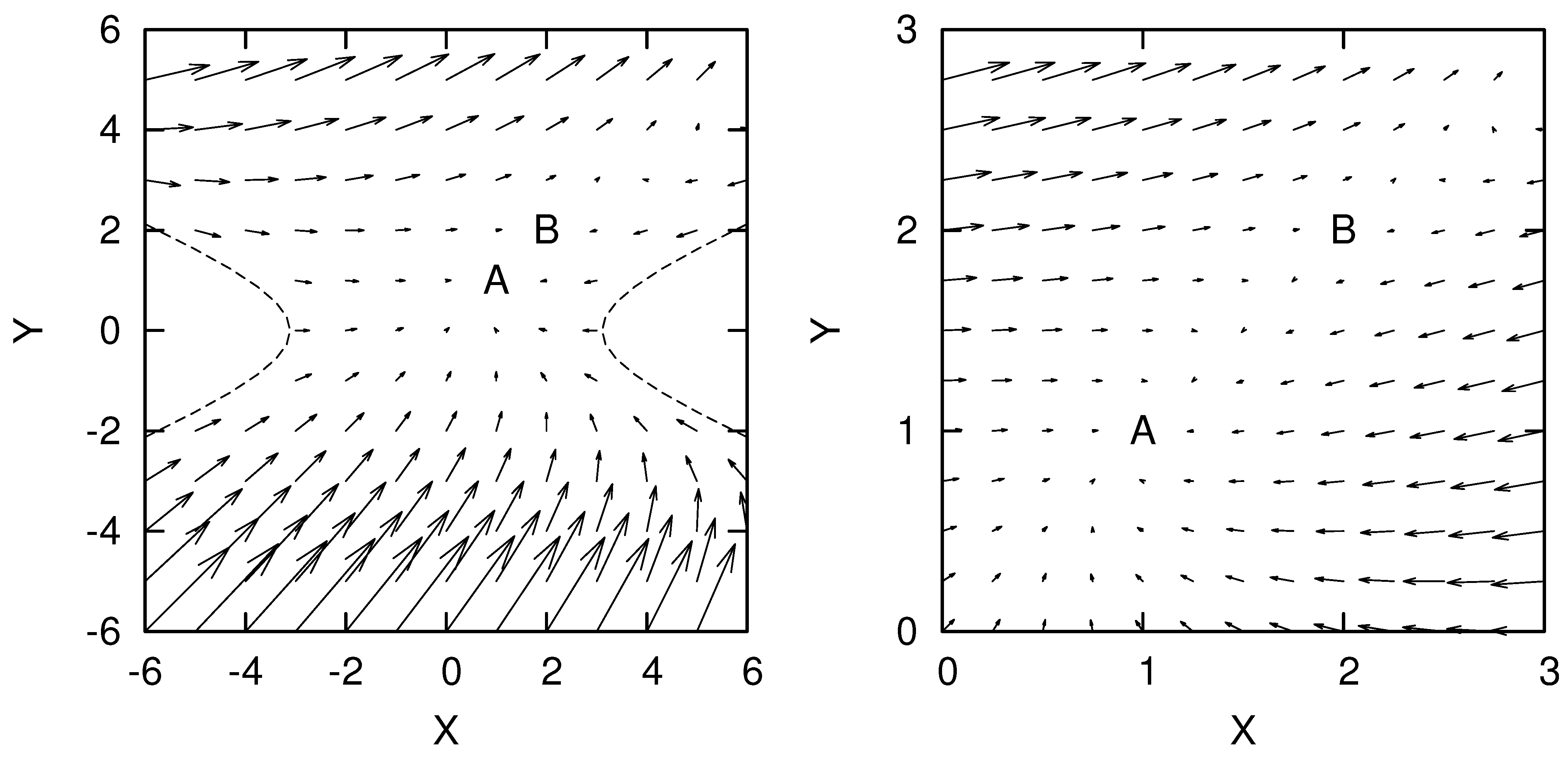
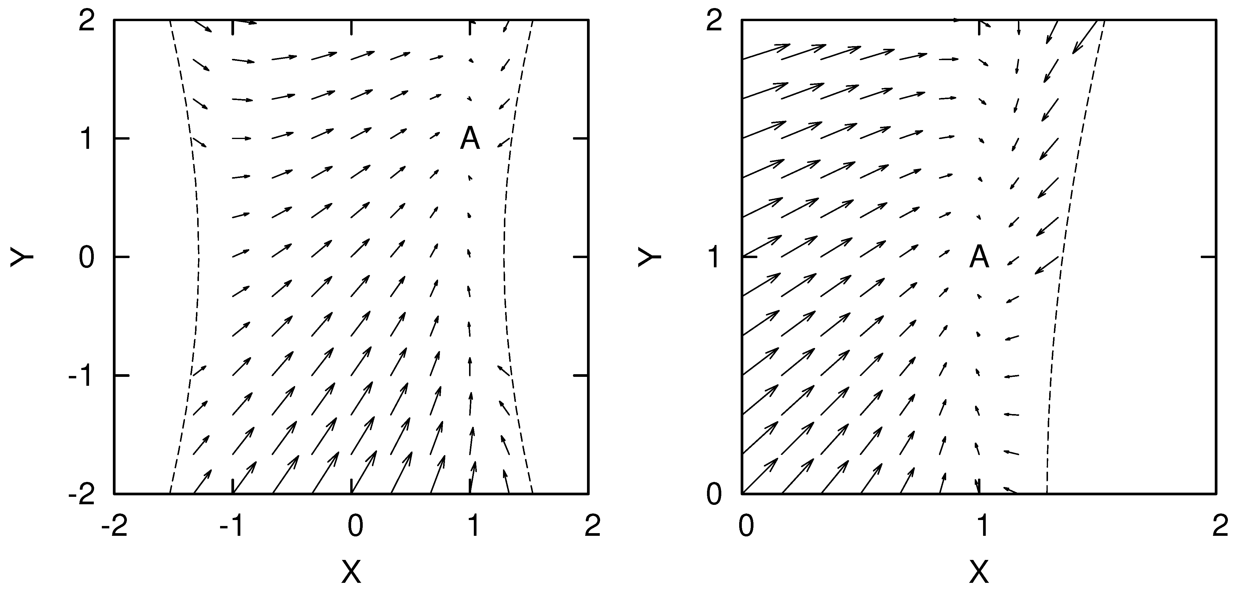
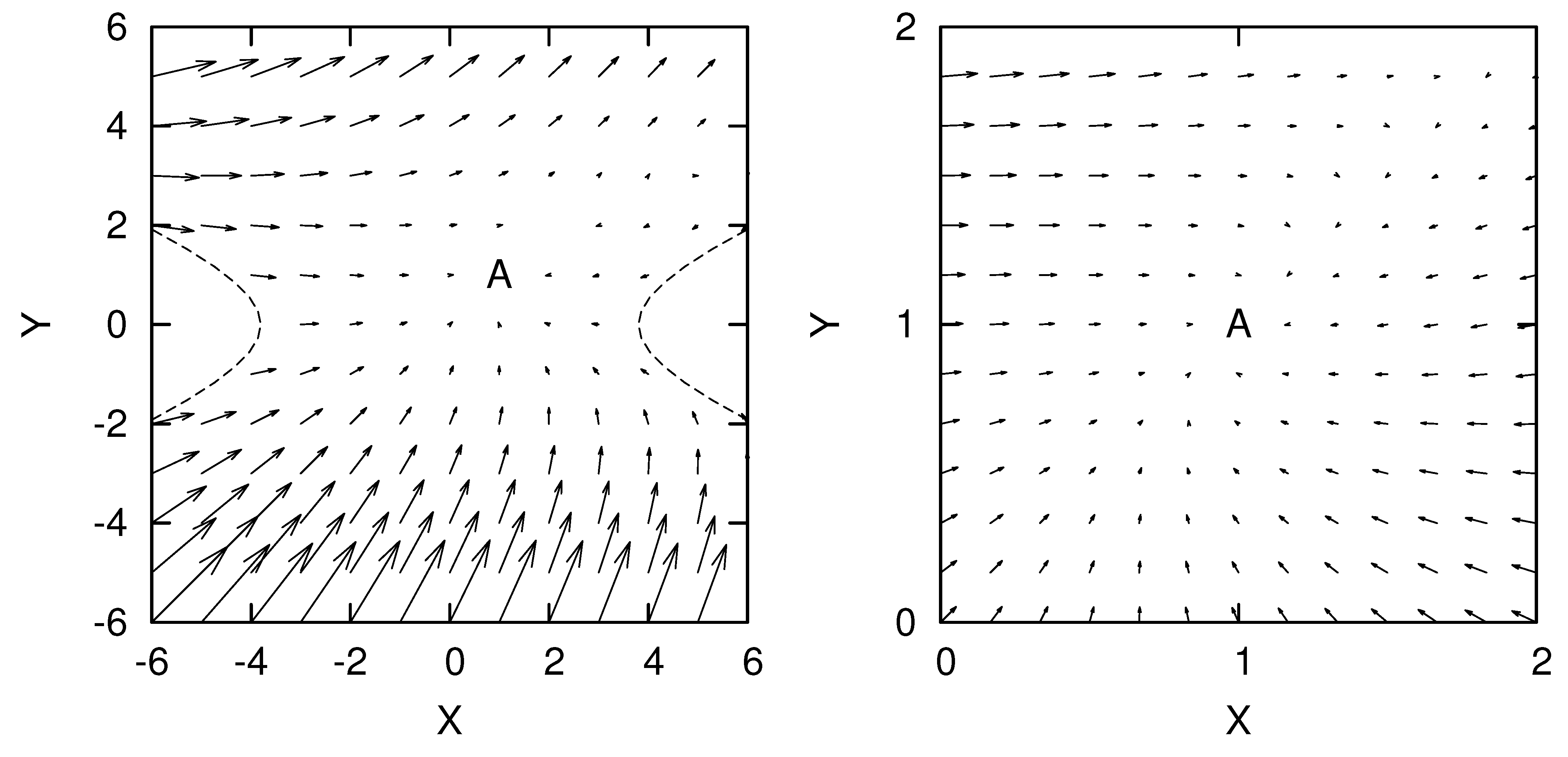
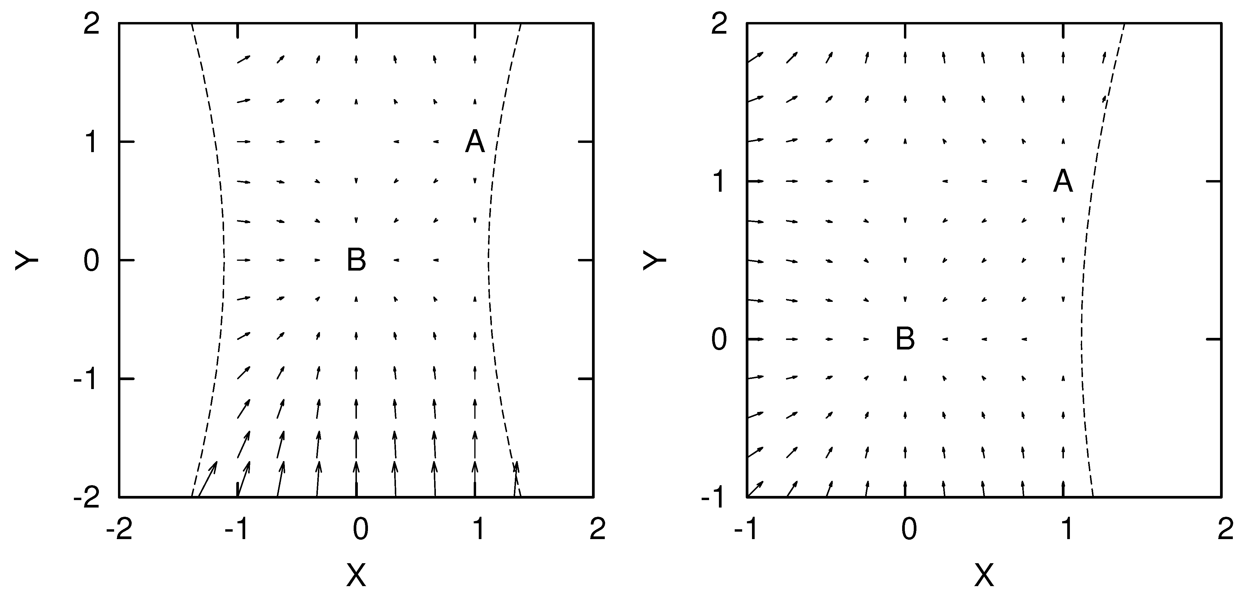
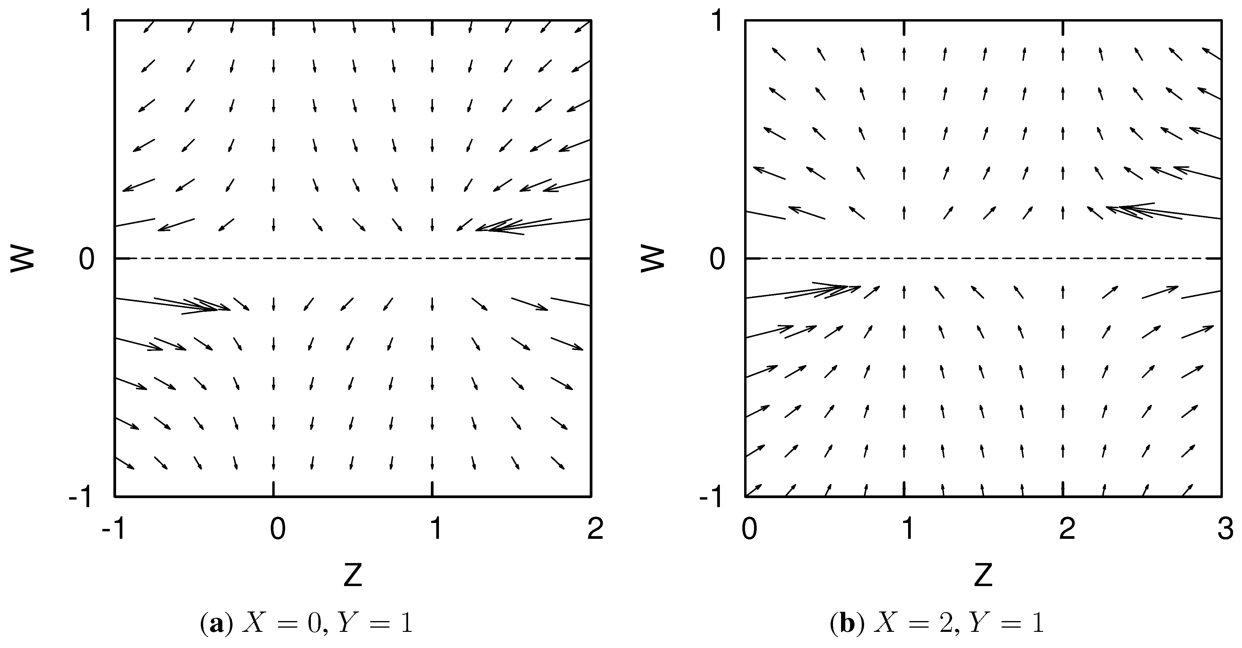
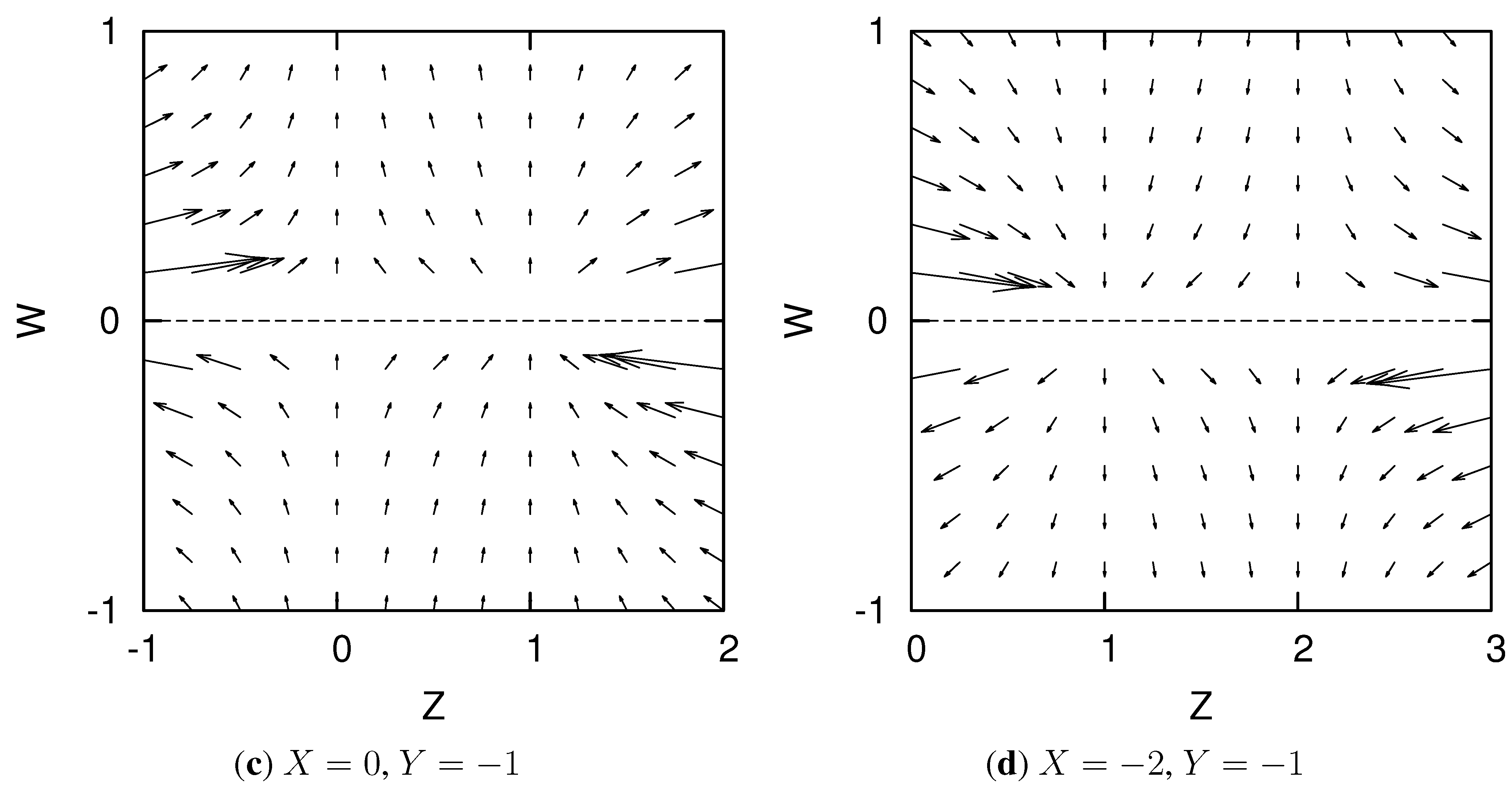
4.2. Fixed Points and Flow of General Solutions

Note that the solution Equation (80) is one of the solutions in the model Equation (18) with Equation (79) and Equation (78). In order to consider the structure of the space of the solutions, by defining dimensionless variables, we investigate the flow of the general solutions. Besides the solution Equation (80), in general, there are other solutions including the one describing the de Sitter space-time corresponding to the extrema of the potential $V(\varphi ,\chi )$, where ϕ and χ are constant. We choose the variables so that both of the solution Equation (80) and the de Sitter solution correspond to fixed points.

Let us introduce the dimensionless variables as follows:

$$X=\kappa {\varphi }^{\prime },Y=\kappa {\chi }^{\prime },Z=\frac{\varphi }{\chi },W=\kappa \left(\varphi -\chi \right)$$

(81)

Equations (74) and (75) are rewritten as

$$\begin{array}{c}\hfill \begin{array}{cc}\hfill X^{\prime }& =3\left(1-X\right)+\frac{1}{2}\omega \left(\varphi (Z,W)\right)\left(X-X^2\right)+\frac{1}{2}\eta \left(\chi (Z,W)\right)\left(X-Y^2\right)\hfill \\ & \phantom{=}+\frac{{\omega }_{,\varphi }\left(\varphi (Z,W)\right)}{2\kappa \omega \left(\varphi \right(Z,W\left)\right)}\frac{6\left(1-X^2\right)-\eta \left(\chi (Z,W)\right)\left(Y^2-X^2\right)}{6-\omega \left(\varphi \right(Z,W\left)\right)-\eta \left(\chi \right(Z,W\left)\right)}\hfill \end{array}\end{array}$$

(82)

$$\begin{array}{c}\hfill \begin{array}{cc}\hfill Y^{\prime }& =3\left(1-Y\right)+\frac{1}{2}\omega \left(\varphi (Z,W)\right)\left(Y-X^2\right)+\frac{1}{2}\eta \left(\chi (Z,W)\right)\left(Y-Y^2\right)\hfill \\ & \phantom{=}+\frac{{\eta }_{,\chi }\left(\chi (Z,W)\right)}{2\kappa \eta \left(\chi \right(Z,W\left)\right)}\frac{6\left(1-Y^2\right)-\omega \left(\varphi (Z,W)\right)\left(X^2-Y^2\right)}{6-\omega \left(\varphi \right(Z,W\left)\right)-\eta \left(\chi \right(Z,W\left)\right)}\hfill \end{array}\end{array}$$

(83)

$$\begin{array}{cc}\hfill Z^{\prime }& =-\frac{\left(X-YZ\right)\left(1-Z\right)}{W}\hfill \end{array}$$

(84)

$$\begin{array}{cc}\hfill W^{\prime }& =X-Y\hfill \end{array}$$

(85)

Now the Hubble rate H is given by

$$H=\frac{\tilde{\mathcal{F}}(\varphi (Z,W),\chi (Z,W))}{\kappa }\sqrt{\frac{6-\omega \left(\varphi \right(Z,W\left)\right)-\eta \left(\chi \right(Z,W\left)\right)}{6-\omega \left(\varphi (Z,W)\right)X^2-\eta \left(\chi (Z,W)\right)Y^2}}$$

(86)

In order for the Hubble rate to be real, the values of X, Y, Z and W are restricted to a region

$$\frac{6-\omega \left(\varphi (Z,W)\right)X^2-\eta \left(\chi (Z,W)\right)Y^2}{6-\omega \left(\varphi \right(Z,W\left)\right)-\eta \left(\chi \right(Z,W\left)\right)}>0$$

(87)

When $\omega \left(\varphi \right)$ and $\eta \left(\chi \right)$ satisfy Equation (78), this system has two fixed points as follows:

Point A 

$(X,Y,Z,W)=(1,1,1,0)$

Here the solution is given by Equation (80).

Point B 

$(X,Y,Z,W)=({\beta }_1,{\beta }_1,1,0)$

Besides Point A $(X,Y,Z,W)=(1,1,1,0)$, there could be another solution for Equations (82–85). In order to show the existence of another solution, we now define $\beta \left(N\right)$ by

$$\beta \left(N\right)\equiv {\beta }_0+{\beta }_{1}N$$

(88)

Here ${\beta }_0$ and ${\beta }_1$ are dimensionless constants. We now assume that the following equation could be satisfied,

$$\frac{{\omega }_{,\varphi }(\beta \left(N\right)/\kappa )}{\kappa \omega \left(\beta \right(N)/\kappa )}=\frac{{\eta }_{,\chi }(\beta \left(N\right)/\kappa )}{\kappa \eta \left(\beta \right(N)/\kappa )}=-\frac{6}{1+{\beta }_1}\left[1+\frac{f^{\prime }\left(\beta \left(N\right)\right)}{3f\left(\beta \right(N\left)\right)}\right]\left[1-\frac{f^{\prime }\left(\beta \left(N\right)\right)}{3f\left(\beta \right(N\left)\right)}{\beta }_1\right]$$

(89)

Then if there exist ${\beta }_0$ and ${\beta }_1$ which satisfy Equation (89), we find Equations (82–85) is satisfied by the following solution:

$$\varphi =\chi =\frac{\beta \left(N\right)}{\kappa },H=\frac{f\left(\beta \right(N\left)\right)}{\kappa }\sqrt{\frac{3f\left(\beta \left(N\right)\right)+f^{\prime }\left(\beta \left(N\right)\right)}{3f\left(\beta \left(N\right)\right)+{\beta }_1{}^2{f}^{\prime }\left(\beta \left(N\right)\right)}}$$

(90)

Especially when ${\beta }_1=0$, this point describes de Sitter space-time.

We now choose $\omega \left(\varphi \right)$ and $\eta \left(\chi \right)$ as

$$\omega \left(\varphi \right)=-\frac{f^{\prime }\left(\kappa \varphi \right)-\sqrt{f^{\prime }{\left(\kappa \varphi \right)}^2+\alpha {\left(\kappa \varphi \right)}^2}}{f\left(\kappa \varphi \right)}>0,\eta \left(\chi \right)=-\frac{f^{\prime }\left(\kappa \chi \right)+\sqrt{f^{\prime }{\left(\kappa \chi \right)}^2+\alpha {\left(\kappa \chi \right)}^2}}{f\left(\kappa \chi \right)}<0$$

(91)

where $\alpha \left(N\right)$ is an arbitrary function. If we choose $\alpha \left(N\right)={\tilde{\alpha }}_0{\mathcal{F}}^{\prime }\left(N\right)$ and $\mathcal{F}\left(N\right)$ being a monotonically increasing or decreasing function, $\omega \left(\varphi \right)$ and $\eta \left(\chi \right)$ are respectively given by

$$\omega \left(\varphi \right)=-\left(1-ϵ\sqrt{1+{\tilde{\alpha }}_0{}^2}\right)\frac{f^{\prime }\left(\kappa \varphi \right)}{f\left(\kappa \varphi \right)},\eta \left(\chi \right)=-\left(1+ϵ\sqrt{1+{\tilde{\alpha }}_0{}^2}\right)\frac{f^{\prime }\left(\kappa \chi \right)}{f\left(\kappa \chi \right)}$$

(92)

Here ${\tilde{\alpha }}_0$ is a dimensionless constant and $ϵ\equiv {\mathcal{F}}^{\prime }\left(N\right)/\left|{\mathcal{F}}^{\prime }\left(N\right)\right|$. Then $V(\varphi ,\chi )$ has the following form:

$$\begin{array}{cc}\hfill V(\varphi ,\chi )& =\frac{3}{{\kappa }^4}f{\left(\kappa \varphi \right)}^{1-ϵ\sqrt{1+{\tilde{\alpha }}_0{}^2}}f{\left(\kappa \chi \right)}^{1+ϵ\sqrt{1+{\tilde{\alpha }}_0{}^2}}\hfill \\ & \phantom{=}\times \left[1+\frac{1-ϵ\sqrt{1+{\tilde{\alpha }}_0{}^2}}{6}\frac{f^{\prime }\left(\kappa \varphi \right)}{f\left(\kappa \varphi \right)}+\frac{1+ϵ\sqrt{1+{\tilde{\alpha }}_0{}^2}}{6}\frac{f^{\prime }\left(\kappa \chi \right)}{f\left(\kappa \chi \right)}\right]\hfill \end{array}$$

(93)

4.2.1. Model with Exponential Growth

As an example, we consider

$$\mathcal{F}\left(N\right)=f_0{\mathrm{e}}^{\tilde{\lambda }N}$$

(94)

where $\tilde{\lambda }$ is a dimensionless constant. Equation (93) has a solution $H\left(N\right)=f_0{\mathrm{e}}^{\tilde{\lambda }N}/\kappa$. Then $\omega \left(\varphi \right)$ and $\eta \left(\chi \right)$ are given by

$$\omega \left(\varphi \right)=-\left(1-ϵ\sqrt{1+{\tilde{\alpha }}_0{}^2}\right)\tilde{\lambda },\eta \left(\chi \right)=-\left(1+ϵ\sqrt{1+{\tilde{\alpha }}_0{}^2}\right)\tilde{\lambda }$$

(95)

and $V(\varphi ,\chi )$ is:

$$V(\varphi ,\chi )=\frac{3f_0{}^2}{{\kappa }^4}\left(1+\frac{\tilde{\lambda }}{3}\right)exp\left[\left(1-ϵ\sqrt{1+{\tilde{\alpha }}_0{}^2}\right)\tilde{\lambda }\kappa \varphi +\left(1+ϵ\sqrt{1+{\tilde{\alpha }}_0{}^2}\right)\tilde{\lambda }\kappa \chi \right]$$

(96)

The EoS parameter of the point A is

$$w=-1-\frac{2}{3}\tilde{\lambda }$$

(97)

which is independent of N. If $\tilde{\lambda }>0$, the point B exists and is located in $(3/\tilde{\lambda },3/\tilde{\lambda },1,0)$. Then the solution is given by

$$\varphi =\chi =\frac{3\left(N-N_0\right)}{\tilde{\lambda }\kappa },H=\frac{f_0}{\kappa }\sqrt{\frac{\tilde{\lambda }}{3}}{\mathrm{e}}^{3\left(N-N_0\right)}$$

(98)

Here $N_0$ is an arbitrary constant. The EoS parameter of this point is $-3$. In this model, the dynamics of X and Y are independent of Z and W. Therefore, we consider a small fluctuation from each fixed point by

$$X\left(N\right)=X_0+\delta X\left(N\right),Y\left(N\right)=Y_0+\delta Y\left(N\right)$$

(99)

Here $X_0$ and $Y_0$ are the values of X and Y in each fixed point. Then Equations (82) and (83) have the following form:

$$\frac{d}{dN}\left(\begin{array}{c}\delta X\\ \delta Y\end{array}\right)=\left(\begin{array}{cc}-3-\tilde{\lambda }+\left(1-ϵ\sqrt{1+{\tilde{\alpha }}_0{}^2}\right)\tilde{\lambda }{X}_0& \left(1+ϵ\sqrt{1+{\tilde{\alpha }}_0{}^2}\right)\tilde{\lambda }{Y}_0\\ \left(1-ϵ\sqrt{1+{\tilde{\alpha }}_0{}^2}\right)\tilde{\lambda }{X}_0& -3-\tilde{\lambda }+\left(1+ϵ\sqrt{1+{\tilde{\alpha }}_0{}^2}\right)\tilde{\lambda }{Y}_0\end{array}\right)\left(\begin{array}{c}\delta X\\ \delta Y\end{array}\right)$$

(100)

The eigenvalues of this matrix Equation (100) are given by

$${\sigma }_1=-3-\tilde{\lambda },{\sigma }_2=-3-\tilde{\lambda }+\left(1-ϵ\sqrt{1+{\tilde{\alpha }}_0{}^2}\right)\tilde{\lambda }{X}_0+\left(1+ϵ\sqrt{1+{\tilde{\alpha }}_0{}^2}\right)\tilde{\lambda }{Y}_0$$

(101)

These indicate that the point A is stable if $-3<\tilde{\lambda }<3$ and unstable if $\tilde{\lambda }<-3$ or $\tilde{\lambda }>3$. Similarly, the point B is stable if $\tilde{\lambda }>3$ and unstable if $0<\tilde{\lambda }<3$. The dynamics of X and Y are shown in Figure 1 and Figure 2.

Figure 1. Each vector denotes $(X^{\prime }/50,Y^{\prime }/50)$, which is independent of Z and W. The parameters are $\tilde{\lambda }=3/2$ and ${\tilde{\alpha }}_0=1$. The point A is located in $(1,1)$, where the EoS parameter is $-2$. The point B is located in $(2,2)$, where the EoS parameter is $-3$.

Figure 1. Each vector denotes $(X^{\prime }/50,Y^{\prime }/50)$, which is independent of Z and W. The parameters are $\tilde{\lambda }=3/2$ and ${\tilde{\alpha }}_0=1$. The point A is located in $(1,1)$, where the EoS parameter is $-2$. The point B is located in $(2,2)$, where the EoS parameter is $-3$.

Figure 2. Each vector denotes $(X^{\prime }/20,Y^{\prime }/20)$, which is independent of Z and W. The parameters are $\tilde{\lambda }=-3/2$ and ${\tilde{\alpha }}_0=1$. The point A is located in $(1,1)$, where the EoS parameter is 0.

Figure 2. Each vector denotes $(X^{\prime }/20,Y^{\prime }/20)$, which is independent of Z and W. The parameters are $\tilde{\lambda }=-3/2$ and ${\tilde{\alpha }}_0=1$. The point A is located in $(1,1)$, where the EoS parameter is 0.

4.2.2. Little Rip Model

We now consider another example

$$\mathcal{F}\left(N\right)=f_0{N}^{\gamma }$$

(102)

where γ is a dimensionless constant. We should note that the case $\gamma =1$ corresponds to the Little Rip model Equation (34). Then $\omega \left(\varphi \right)$ and $\eta \left(\chi \right)$ are given by

$$\omega \left(\varphi \right)=-\left(1-ϵ\sqrt{1+{\tilde{\alpha }}_0{}^2}\right)\frac{\gamma }{\kappa \varphi },\eta \left(\chi \right)=-\left(1+ϵ\sqrt{1+{\tilde{\alpha }}_0{}^2}\right)\frac{\gamma }{\kappa \chi }$$

(103)

and $V(\varphi ,\chi )$ has the following form:

$$\begin{array}{cc}\hfill V(\varphi ,\chi )& =\frac{3f_0{}^2}{{\kappa }^4}{\left(\kappa \varphi \right)}^{1-ϵ\sqrt{1+{\tilde{\alpha }}_0{}^2}}{\left(\kappa \chi \right)}^{1+ϵ\sqrt{1+{\tilde{\alpha }}_0{}^2}}\hfill \\ & \phantom{=}\times \left[1+\frac{1-ϵ\sqrt{1+{\tilde{\alpha }}_0{}^2}}{6}\frac{\gamma }{\kappa \varphi }+\frac{1+ϵ\sqrt{1+{\tilde{\alpha }}_0{}^2}}{6}\frac{\gamma }{\kappa \chi }\right]\hfill \end{array}$$

(104)

The EoS parameter of the point A is

$$w=-1-\frac{2\gamma }{3N}$$

(105)

which becomes $-1$ when $N\to \infty$. If $\gamma <1/2$, the point B exists and is located in $(0,0,1,0)$. Then the solution is

$$\varphi =\chi =\frac{1-2\gamma }{6\kappa },H=\frac{f_0}{\sqrt{6}\kappa }{\left(\frac{6}{1-2\gamma }\right)}^{1/2-\gamma }$$

(106)

This point corresponds to the de Sitter space-time. We consider a small fluctuation from the point B by

$$\varphi \left(N\right)=\frac{1-2\gamma }{6\kappa }+\delta \varphi \left(N\right),\chi \left(N\right)=\frac{1-2\gamma }{6\kappa }+\delta \chi \left(N\right)$$

(107)

Then Equations (82) and (83) have the following form:

$$\begin{array}{cc}\hfill 0=& \left(1-2\gamma \right)\frac{d^2}{d{N}^2}\left(\begin{array}{c}\delta \varphi \\ \delta \chi \end{array}\right)+3\frac{d}{dN}\left(\begin{array}{c}\delta \varphi \\ \delta \chi \end{array}\right)\hfill \\ & -18\left(\begin{array}{cc}1-\left(1-ϵ\sqrt{1+{\tilde{\alpha }}_0{}^2}\right)\gamma & -\left(1+ϵ\sqrt{1+{\tilde{\alpha }}_0{}^2}\right)\gamma \\ -\left(1-ϵ\sqrt{1+{\tilde{\alpha }}_0{}^2}\right)\gamma & 1-\left(1+ϵ\sqrt{1+{\tilde{\alpha }}_0{}^2}\right)\gamma \end{array}\right)\left(\begin{array}{c}\delta \varphi \\ \delta \chi \end{array}\right)\hfill \end{array}$$

(108)

The solution of this Equation (108) is given by

$$\left(\begin{array}{c}\delta \varphi \\ \delta \chi \end{array}\right)=\left(\begin{array}{c}1+ϵ\sqrt{1+{\tilde{\alpha }}_0{}^2}\\ -1+ϵ\sqrt{1+{\tilde{\alpha }}_0{}^2}\end{array}\right)\frac{C_{1+}{\mathrm{e}}^{{\sigma }_{1+}N}+C_{1-}{\mathrm{e}}^{{\sigma }_{1-}N}}{\kappa }+\left(\begin{array}{c}1\\ 1\end{array}\right)\frac{C_{2+}{\mathrm{e}}^{{\sigma }_{2+}N}+C_{2-}{\mathrm{e}}^{{\sigma }_{2-}N}}{\kappa }$$

(109)

Here $C_{1\pm }$ and $C_{2\pm }$ are arbitrary constants and ${\sigma }_{1\pm }$ and ${\sigma }_{2\pm }$ are given by

$${\sigma }_{1\pm }=\frac{-3\pm 3\sqrt{1+8\left(1-2\gamma \right)}}{2\left(1-2\gamma \right)},{\sigma }_{2\pm }=\frac{-3\pm 3\sqrt{1+8\left(1-2\gamma \right){}^2}}{2\left(1-2\gamma \right)}$$

(110)

Since ${\sigma }_{1+}$ and ${\sigma }_{1-}$ are positive, Equation (109) tells that the fluctuation grows up when N increases, which tells that the point B is unstable. On the other hand, when ϕ, $\chi \to \infty$, X and Y in the solution behave as

$$X=1-X_1{\mathrm{e}}^{-3N},Y=1-Y_1{\mathrm{e}}^{-3N}$$

(111)

Here $X_1$ and $Y_1$ are arbitrary constants. This indicates that the values of X and Y approach to $(1,1)$ if ϕ, $\chi \to \infty$ when $N\to \infty$. Then the Hubble rate approaches to $f_0{N}^{\gamma }/\kappa$, which corresponds to the Little Rip universe if $\gamma =1$. The dynamics of X and Y are shown in Figure 3 and Figure 4 and those of W and Z are in Figure 5.

Figure 3. Each vector denotes $(X^{\prime }/50,Y^{\prime }/50)$ with $Z=1$ and $W=0$ ($\varphi =\chi =1/\kappa$). The parameters are $\gamma =1$ and ${\tilde{\alpha }}_0=1$. The point A is located in $(1,1)$, which corresponds to the Little Rip universe.

Figure 3. Each vector denotes $(X^{\prime }/50,Y^{\prime }/50)$ with $Z=1$ and $W=0$ ($\varphi =\chi =1/\kappa$). The parameters are $\gamma =1$ and ${\tilde{\alpha }}_0=1$. The point A is located in $(1,1)$, which corresponds to the Little Rip universe.

Figure 4. Each vector denotes $(X^{\prime }/20,Y^{\prime }/20)$ with $Z=1$ and $W=0$ ($\varphi =\chi =1/2\kappa$). The parameters are $\gamma =-1$ and ${\tilde{\alpha }}_0=1$. The point A is located in $(1,1)$. The point B is located in $(0,0)$, which corresponds to the de Sitter universe.

Figure 4. Each vector denotes $(X^{\prime }/20,Y^{\prime }/20)$ with $Z=1$ and $W=0$ ($\varphi =\chi =1/2\kappa$). The parameters are $\gamma =-1$ and ${\tilde{\alpha }}_0=1$. The point A is located in $(1,1)$. The point B is located in $(0,0)$, which corresponds to the de Sitter universe.

Figure 5. Each vector denotes $(Z^{\prime }/20,W^{\prime }/20)$, which is independent of the form of $\omega \left(\varphi \right)$, $\eta \left(\chi \right)$ and $V(\varphi ,\chi )$. The dynamics of Z and W are classified into four types according to the values of X and Y as (a) $0<Y$, $X<Y$; (b) $0<Y<X$; (c) $0>Y$, $X>Y$ and (d) $0>Y>X$. The fixed points are located in $(1,0)$.

Figure 5. Each vector denotes $(Z^{\prime }/20,W^{\prime }/20)$, which is independent of the form of $\omega \left(\varphi \right)$, $\eta \left(\chi \right)$ and $V(\varphi ,\chi )$. The dynamics of Z and W are classified into four types according to the values of X and Y as (a) $0<Y$, $X<Y$; (b) $0<Y<X$; (c) $0>Y$, $X>Y$ and (d) $0>Y>X$. The fixed points are located in $(1,0)$.

As mentioned above, the model Equation (102) with $\gamma =1$ corresponds to the Little Rip model Equation (34). In fact, Equation (34) indicates that

$$N=\frac{H_0^{\left(\mathrm{I}\right)}}{\lambda }{\mathrm{e}}^{\lambda t}$$

(112)

and therefore

$$H=\lambda N$$

(113)

By comparing Equation (113) with Equation (102), we find $f_0=\lambda$. Then as written after Equation (35), the parameter $f_0$ is bounded as $2.37\times {10}^{-3}{\text{Gyr}}^{-1}\le f_0\le 8.37\times {10}^{-3}{\text{Gyr}}^{-1}$ by the results of the Supernova Cosmology Project [41]. If we choose so that the present universe corresponds to $N=N_0$, we have $f_0{N}_0\sim 70\text{km}/\mathrm{s}\text{Mpc}$.

4.3. The Potential and the (in)stability

Hence, we have completed the formulation of the reconstruction in terms of the e-foldings. The e-foldings description is directly related with redshift and therefore with the cosmological observations. We also investigated the flow for the solution, which shows the (in)stability of the reconstructed solution obtained in a large range. Even if the solution is stable, when the stability region is small, the evolution of the universe depends strongly on the initial conditions. If the initial condition is out of the range, the universe does not always evolve to the solution obtained by the reconstruction. On the other hand, if the stable region is large enough, even if the universe started from an initial condition in a rather large region, the universe evolves to the solution obtained by the reconstruction. The size of the stable region depend on the choice of α in Equation (22). In other words, we may control the size of the stable region. Anyway for more quantitative analysis, we may need numerical calculation, which could be one of the future works.

In case of the canonical scalar field as χ, usually the scalar field rolls down the potential. In case of the phantom scalar field as ϕ, the scalar field climbs up the potential. This phenomenon occurs due to the non-canonical kinetic term. For the canonical scalar field ${\phi }_c$, the field equation has the form of ${\nabla }_t^2{\phi }_c=-V^{\prime }\left(\varphi \right)$ but for the phantom scalar field ${\phi }_p$, the sign of the kinetic term is changed, and we obtain ${\nabla }_t^2{\phi }_p=V^{\prime }\left(\varphi \right)$ for a phantom scalar field. That is, the sign of the “force” is effectively changed. Then if there is an extremum in the potential, which corresponds to the de Sitter space-time, the de Sitter solution can be stable if the extremum corresponds to the minimum in χ and the maximum of ϕ; otherwise the de Sitter solution is unstable and the space-time could evolve to other solution by a small perturbation. The Rip generally occurs when the scalar fields climb up the potential and the energy density of the scalar fields becomes larger and larger. If the scalar fields arrive at the infinity of the potential in a finite time, there occurs the Big Rip, but if they arrive at the infinity when the cosmological time t goes to infinity, there occurs the Little Rip. Then the solution corresponding to the Big/Little Rip is stable, there is a path going to the infinity of the potential and the path is minimum for the scalar field χ. Otherwise the universe may evolve to other solution.

5. Discussion

In summary, we gave a general formulation of reconstruction in two scalar model and investigated the stability of the solution. This formulation helped us to construct a model which has a stable cosmological solution describing the phantom-divide crossing. By using the formulation, we constructed non-singular phantom model which describes the cosmological solutions with and without Little Rip and investigated the (in)stability of the solutions. The existence of the solution describing (asymptotically) de Sitter space-time was also investigated and furthermore the stability of the de Sitter solution when it exists as well as possible transition of Little Rip cosmology to de Sitter one were investigated. We also considered the reconstruction of the two scalar model in terms of the e-foldings N and investigated the flow of the solution by defining the dimensionless variables, which give the fixed points for some solutions.

Finally, let us make several remarks about the relation of the qualitative behavior of the Universe evolution and the shape of the scalar potential.

In case of the usual canonical scalar field as ϕ in Equation (18), when the field climbs up the potential, the kinetic energy decreases until the kinetic energy vanishes. Even in case of the phantom field as χ in Equation (18) with non-canonical kinetic term, the kinetic energy decreases when the field climbs up the potential. In case of the phantom field, the kinetic energy is unbounded below and therefore the absolute value of the kinetic energy increases when the field climbs up the potential. The Big Rip or Little Rip occurs when the potential goes to infinity. If the potential tends to infinity in the finite future, the evolution corresponds to the Big Rip, but if the potential goes to infinity in the infinite future, the evolution corresponds to the Little Rip. Then the necessary condition that the Big or Little Rip could occur is

(1)

The potential does not have maximum and it goes to infinity.

(2)

There is a path in the potential that the potential becomes infinite but the kinetic energy of the canonical scalar field is vanishing.

Since we identify the scalar field ϕ and χ with the cosmological time, the second condition means $\omega \left(\varphi \right)$ in Equation (18) goes to zero when ϕ goes to infinity and therefore the phantom field χ dominates. Conversely, if there is a maximum in the potential or there is no path in the potential that the potential becomes infinite but the kinetic energy of the canonical scalar field goes to zero, there does not occur big rip nor Little Rip.

Let us suppose the case that there is a maximum in the potential. If the fields stay near the potential maximum, the universe becomes asymptotically de Sitter space-time. If the fields go through the maximum and the potential decreases, the kinetic energy of the canonical scalar field increases but the absolute value of the kinetic energy of the phantom field decreases. If the kinetic energy of the phantom field goes to zero, the canonical field becomes dominant and the Universe could enter the non-phantom (quintessence) phase and there might occur the deceleration phase in future.

In order to explain the accelerating expansion of the present universe, many kinds of models have been proposed. As clear even in this paper, only from the history of the expansion, we cannot find which model could be a real one. In order to distinguish between different models, the cosmological perturbation could be an important tool, which could be also one of the future works. Some works to distinguish between different models have been already reported in [9], for example.

References

1. De Bernardis, P.; Ade, P.A.R.; Bock, J.J.; Bond, J.R.; Borrill, J.; Boscaleri, A.; Coble, K.; Crill, B.P.; de Gasperis, G.; Farese, P.C.; et al. A flat universe from high resolution maps of the cosmic microwave background radiation. Nature 2000, 404, 955–959. [Google Scholar] [CrossRef] [PubMed]
2. Hanany, S.; Ade, P.; Balbi, A.; Bock, J.; Borrill, J.; Boscaleri, A.; de Bernardis, P.; Ferreira, P.G.; Hristov, V.V.; Jaffe, A.H.; et al. MAXIMA-1: A measurement of the cosmic microwave background anisotropy on angular scales of 10 arcminutes to 5 degrees. Astrophys. J. 2000, 545. [Google Scholar] [CrossRef]
3. Perlmutter, S.; Aldering, G.; Goldhaber, G.; Knop, R.A.; Nugent, P.; Castro, P.G.; Deustua, S.; Fabbro, S.; Goobar, A.; Groom, D.E.; et al. Measurements of omega and lambda from 42 high redshift supernovae. Astrophys. J. 1999, 517, 565–586. [Google Scholar] [CrossRef]
4. Perlmutter, S.; Aldering, G.; Della Valle, M.; Deustua, S.; Ellis, R.S.; Fabbro, S.; Fruchter, A.; Goldhaber, G.; Goobar, A.; Groom, D.E.; et al. Discovery of a supernova explosion at half the age of the Universe and its cosmological implications. Nature 1998, 391, 51–54. [Google Scholar] [CrossRef]
5. Riess, A.G.; Filippenko, A.V.; Challis, P.; Clocchiattia, A.; Diercks, A.; Garnavich, P.M.; Gilliland, R.L.; Hogan, C.J.; Jha, S.; Kirshner, R.P.; et al. Observational evidence from supernovae for an accelerating universe and a cosmological constant. Astron. J. 1998, 116, 1009–1038. [Google Scholar] [CrossRef]
6. Silvestri, A.; Trodden, M. Approaches to understanding cosmic acceleration. Rep. Prog. Phys. 2009, 72. [Google Scholar] [CrossRef]
7. Li, M.; Li, X.-D.; Wang, S.; Wang, Y. Dark energy. Commun. Theor. Phys. 2011, 56, 525–604. [Google Scholar] [CrossRef]
8. Caldwell, R.R.; Kamionkowski, M. The physics of cosmic acceleration. Ann. Rev. Nucl. Part. Sci. 2009, 59, 397–429. [Google Scholar] [CrossRef]
9. Copeland, E.J.; Sami, M.; Tsujikawa, S. Dynamics of dark energy. Int. J. Mod. Phys. 2006, D15, 1753–1936. [Google Scholar] [CrossRef]
10. Clifton, T.; Ferreira, P.G.; Padilla, A.; Skordis, C. Modified gravity and cosmology. Phys. Rep. 2012, 513, 1–189. [Google Scholar] [CrossRef]
11. Conley, A.; Guy, J.; Sullivan, M.; Regnault, N.; Astier, P.; Balland, C.; Basa, S.; Carlberg, R.G.; Fouchez, D.; Hardin, D.; et al. Supernova constraints and systematic uncertainties from the first 3 years of the supernova legacy survey. Astrophys. J. Suppl. 2011, 192, 1–29. [Google Scholar] [CrossRef]
12. Sullivan, M.; Guy, J.; Conley, A.; Regnault, N.; Astier, P.; Balland, C.; Basa, S.; Carlberg, R.G.; Fouchez, D.; Hardin, D.; et al. SNLS3: Constraints on dark energy combining the supernova legacy survey three year data with other probes. Astrophys. J. 2011, 737. [Google Scholar] [CrossRef]
13. Komatsu, E.; Smith, K.M.; Dunkley, J.; Bennett, C.L.; Gold, B.; Hinshaw, G.; Jarosik, N.; Larson, D.; Nolta, M.R.; Page, L.; et al. Seven-year Wilkinson Microwave Anisotropy Probe (WMAP) observations: Cosmological interpretation. Astrophys. J. Suppl. 2011, 192. [Google Scholar] [CrossRef]
14. Dunkley, J.; Hlozek, R.; Sievers, J.; Acquaviva, V.; Ade, P.A.R.; Aguirre, P.; Amiri, M.; Appel, J.W.; et al. The atacama cosmology telescope: Cosmological parameters from the 2008 power spectra. Astrophys. J. 2011, 739. [Google Scholar] [CrossRef]
15. Reid, B.A.; Percival, W.J.; Eisenstein, D.J.; Verde, L.; Spergel, D.N.; Skibba, R.A.; Bahcall, N.A.; Budavari, T.; et al. Cosmological constraints from the clustering of the sloan digital sky survey DR7 luminous red galaxies. Mon. Not. R. Astron. Soc. 2010, 404, 60–85. [Google Scholar] [CrossRef] [Green Version]
16. Giannantonio, T.; Scranton, R.; Crittenden, R.G.; Nichol, R.C.; Boughn, S.P.; Myers, A.D.; Richards, G.T. Combined analysis of the integrated Sachs-Wolfe effect and cosmological implications. Phys. Rev. 2008, D77. [Google Scholar] [CrossRef]
17. Ho, S.; Hirata, C.; Padmanabhan, N.; Seljak, U.; Bahcall, N. Correlation of CMB with large-scale structure: I. ISW tomography and cosmological implications. Phys. Rev. 2008, D78. [Google Scholar] [CrossRef]
18. Caldwell, R.R.; Kamionkowski, M.; Weinberg, N.N. Phantom energy and cosmic doomsday. Phys. Rev. Lett. 2003, 91. [Google Scholar] [CrossRef]
19. Nojiri, S.; Odintsov, S.D.; Tsujikawa, S. Properties of singularities in (phantom) dark energy universe. Phys. Rev. 2005, D71. [Google Scholar] [CrossRef]
20. Barrow, J.D. Sudden future singularities. Class. Quantum Grav. 2004, 21, L79–L82. [Google Scholar] [CrossRef]
21. Barrow, J.D. More general sudden singularities. Class. Quantum Grav. 2004, 21, 5619–5622. [Google Scholar] [CrossRef]
22. Nojiri, S.; Odintsov, S.D. Unified cosmic history in modified gravity: From F(R) theory to Lorentz non-invariant models. Phys. Rep. 2011, 505, 59–144. [Google Scholar] [CrossRef]
23. Frampton, P.H.; Ludwick, K.J.; Scherrer, R.J. The little rip. Phys. Rev. 2011, D84, 063003. [Google Scholar] [CrossRef]
24. Frampton, P.H.; Ludwick, K.J.; Nojiri, S.; Odintsov, S.D.; Scherrer, R.J. Models for little rip dark energy. Phys. Lett. 2012, B708, 204–211. [Google Scholar] [CrossRef]
25. Nojiri, S.; Odintsov, S.D.; Saez-Gomez, D. Cyclic, ekpyrotic and little rip universe in modified gravity. AIP Conf. Proc. 2011, 1458, 207–221. [Google Scholar]
26. Brevik, I.; Elizalde, E.; Nojiri, S.; Odintsov, S.D. Viscous little rip cosmology. Phys. Rev. 2011, D84, 103508:1–103508:6. [Google Scholar] [CrossRef]
27. Frampton, P.H.; Ludwick, K.J. Seeking evolution of dark energy. Eur. Phys. J. 2011, C71. [Google Scholar] [CrossRef]
28. Granda, L.N.; Loaiza, E. Big Rip and Little Rip solutions in scalar model with kinetic and Gauss Bonnet couplings. Int. J. Mod. Phys. 2012, D2. [Google Scholar] [CrossRef]
29. Capozziello, S.; de Laurentis, M.; Nojiri, S.; Odintsov, S.D. Classifying and avoiding singularities in the alternative gravity dark energy models. Phys. Rev. 2009, D79. [Google Scholar] [CrossRef]
30. Frampton, P.H.; Ludwick, K.J.; Scherrer, R.J. Pseudo-rip: Cosmological models intermediate between the cosmological constant and the little rip. Phys. Rev. 2012, D85, 083001:1–083001:5. [Google Scholar] [CrossRef]
31. Feng, B.; Wang, X.-L.; Zhang, X.-M. Dark energy constraints from the cosmic age and supernova. Phys. Lett. 2005, B607, 35–41. [Google Scholar]
32. Elizalde, E.; Nojiri, S.; Odintsov, S.D. Late-time cosmology in (phantom) scalar-tensor theory: Dark energy and the cosmic speed-up. Phys. Rev. 2004, D70. [Google Scholar] [CrossRef]
33. Cai, Y.-F.; Saridakis, E.N.; Setare, M.R.; Xia, J.-Q. Quintom cosmology: Theoretical implications and observations. Phys. Rep. 2010, 493, 1–60. [Google Scholar] [CrossRef]
34. Nojiri, S.; Odintsov, S.D. Unifying phantom inflation with late-time acceleration: Scalar phantom-non-phantom transition model and generalized holographic dark energy. Gen. Relativ. Gravit. 2006, 38, 1285–1304. [Google Scholar] [CrossRef]
35. Chimento, L.P.; Forte, M.I.; Lazkoz, R.; Richarte, M.G. Internal space structure generalization of the quintom cosmological scenario. Phys. Rev. 2009, D 79. [Google Scholar] [CrossRef]
36. Nesseris, S.; Perivolaropoulos, L. Crossing the phantom divide: Theoretical implications and observational status. J. Cosmol. Astropart. Phys. 2007, 0701. [Google Scholar] [CrossRef]
37. Capozziello, S.; Nojiri, S.; Odintsov, S.D. Unified phantom cosmology: Inflation, dark energy and dark matter under the same standard. Phys. Lett. 2006, B632, 597–604. [Google Scholar] [CrossRef]
38. Vikman, A. Can dark energy evolve to the phantom? Phys. Rev. 2005, D71. [Google Scholar] [CrossRef]
39. Xia, J.-Q.; Cai, Y.-F.; Qiu, T.-T.; Zhao, G.-B.; Zhang, X. Constraints on the sound speed of dynamical dark energy. Int. J. Mod. Phys. 2008, D17, 1229–1243. [Google Scholar] [CrossRef]
40. Caldwell, R.R. A phantom menace? Phys. Lett. 2002, B545, 23–29. [Google Scholar] [CrossRef]
41. Amanullah, R.; Lidman, C.; Rubin, D.; Aldering, G.; Astier, P.; Barbary, K.; Burns, M.S.; Conley, A.; Dawson, K.S.; Deustua, S.E.; et al. Spectra and light curves of six type Ia supernovae at 0.511 < z < 1.12 and the union2 compilation. Astrophys. J. 2010, 716, 712–738. [Google Scholar]