Kullback–Leibler Divergence Measure for Multivariate Skew-Normal Distributions

Abstract

The aim of this work is to provide the tools to compute the well-known Kullback–Leibler divergence measure for the flexible family of multivariate skew-normal distributions. In particular, we use the Jeffreys divergence measure to compare the multivariate normal distribution with the skew-multivariate normal distribution, showing that this is equivalent to comparing univariate versions of these distributions. Finally, we applied our results on a seismological catalogue data set related to the 2010 Maule earthquake. Specifically, we compare the distributions of the local magnitudes of the regions formed by the aftershocks.

1. Introduction

The first notion of entropy of a probability distribution was addressed by [1], thus becoming a measure widely used to quantify the level of aleatority present on instrumental variables, which has been commonly used in different engineering areas. Posteriorly, several notions of entropies have been proposed in order to generalize the Shannon entropy, such as Rényi entropy and Tsallis entropy. At this time, [2] introduced the so called Kullback–Leibler divergence (KL-divergence) measures, which is a pseudo-distance (or discriminant function) between two probability distributions and the most common divergence measures used in practical works.

In a recent application about polarimetric synthetic aperture radar (PolSAR) images, Frery et al. [3] make use of the complex Wishart distribution (see e.g., [4]) for modeling radar backscatter from forest and pasture areas. There, they conclude that the KL-divergence measure is the best one with respect to Bhattacharyya, Chi-square, Hellinger or Rényi’s distances. The studies in [3] and [4] conclude that it is necessary to have appropriate statistics to compare multivariate distributions such as the Wishart one. In addition, [5] gives an extended theoretical analysis of the most important aspects on information theory for the multivariate normal and Student-t distributions, among other distributions commonly used in the literature. Divergence measures have also been used to examine data influences and model perturbations; see, e.g., [6] for a unified treatment and [7] for a review and some extensions of previous works on Bayesian influence measures based on the KL-divergence. In addition, this measure has been considered in selection model analysis by [8], where the authors recommend this criterion because, in contrast to other criteria such as AIC (Akaike’s Information Criterion), it does not assume the existence of the true model. However, [8] considers the AIC as a good approximation of the KL-divergence for selection model analysis. On the another hand, asymptotic approximations of the KL-divergence for the multivariate linear model are given in [9], whereas asymptotic approximations of the Jeffreys divergence or simply J-divergence for the multivariate linear model are given in [10]. Another example is the Rényi’s divergence and its special case, where the KL-divergence has been recently successfully applied to region-of-interest tracking in video sequences [11], independent subspace analysis [12], image registration [13], and guessing moments [14].

On the other hand, extensive literature has been developed on non-symmetric families of multivariate distributions as the multivariate skew-normal distribution [15,16,17,18]. More recently, a study due to [19] computes the mutual information index of the multivariate skew-normal distribution in terms of an infinite series. Next, this work was extended for the full class of multivariate skew-elliptical distributions by [20], where a real application for optimizing an atmospheric monitoring network is presented using the entropy and mutual information indexes of the multivariate skew-normal, among other related family distributions. Several statistical applications to real problems using multivariate skew-normal distributions and others related families can be found in [21].

In this article, we explore further properties of the multivariate skew-normal distribution. This distribution provides a parametric class of multivariate probability distributions that extends the multivariate normal distribution by an extra vector of parameters that regulates the skewness, allowing for a continuous variation from normality to skew-normality [21]. In an applied context, this multivariate family appears to be very important, since in the multivariate case there are not many distributions available for dealing with non-normal data, primarily when the skewness of the marginals is quite moderate. Considering the multivariate skew-normal distribution as a generalization of the multivariate normal law is a natural choice in all practical situations in which there is some skewness present. For this reason, the main motivation of this article is to analyze some information measures in multivariate observations under the presence of skewness.

Specifically, we propose a theory based on divergence measures for the flexible family of multivariate skew-normal distributions, thus extending the respective theory based on the multivariate normal distribution. For this, we start with the computation of the entropy, cross-entropy, KL-divergence and J-divergence for the multivariate skew-normal distribution. As a byproduct, we use the J-divergence to compare the multivariate skew-normal distribution with the multivariate normal one. Posteriorly, we apply our findings on a seismic catalogue analyzed by [22]. They estimate regions using nonparametric clustering (NPC) methods based on kernel distribution fittings [23], where the spatial location of aftershock events produced by the well-known 2010 earthquake in Maule, Chile is considered. Hence, we compare the skew-distributed local magnitudes among these clusters using KL-divergence and J-divergence; then, we test for significant differences between MLE’s parameter vectors [17].

The organization of this paper is as follows. Section 2 presents general concepts of information theory as entropy, cross-entropy and divergence. Section 3 presents the computation of these concepts for multivariate skew-normal distributions, including the special case of the J-divergence between multivariate skew-normal versus multivariate normal distribution. Section 4 reports numerical results of a real application of seismic events mentioned before and finally, this paper ends with a discussion in Section 5. Some proofs are presented in Appendix A.

2. Entropy and Divergence Measures

Let $\mathbf{Z}\in {\mathbb{R}}^k$ be a random vector with probability density function (pdf) $f_{\mathbf{Z}}\left(\mathbf{z}\right)$. The Shannon entropy—also named differential entropy—which was proposed earlier by [1] is

$$H\left(\mathbf{Z}\right)=-E[log{f}_{\mathbf{Z}}\left(\mathbf{Z}\right)]=-{\int }_{{\mathbb{R}}^k}{f}_{\mathbf{Z}}\left(\mathbf{z}\right)log{f}_{\mathbf{Z}}\left(\mathbf{z}\right)d\mathbf{z}$$

(1)

Here $E\left[g\right(\mathbf{Z}\left)\right]$ denotes the expected information in $\mathbf{Z}$ of the random function $g\left(\mathbf{Z}\right)$. Hence, the Shannon’s entropy is the expected value of $g\left(\mathbf{Z}\right)=-log{f}_{\mathbf{Z}}\left(\mathbf{Z}\right)$, which satisfies $g\left(\mathbf{1}\right)=0$ and $g\left(\mathbf{0}\right)=\infty$.

Suppose now that $\mathbf{X},\mathbf{Y}\in {\mathbb{R}}^k$ are two random vectors with pdf’s $f_{\mathbf{X}}\left(\mathbf{x}\right)$ and $f_{\mathbf{Y}}\left(\mathbf{y}\right)$, respectively, which are assumed to have the same support. Under these conditions, the cross-entropy—also called relative entropy—associated to Shannon entropy (1) is related to compare the information measure of $\mathbf{Y}$ with respect to $\mathbf{X}$, and is defined as follows

$$CH(\mathbf{X},\mathbf{Y})=-E[log{f}_{\mathbf{Y}}\left(\mathbf{X}\right)]=-{\int }_{{\mathbb{R}}^k}{f}_{\mathbf{X}}\left(\mathbf{x}\right)log{f}_{\mathbf{Y}}\left(\mathbf{x}\right)d\mathbf{x}$$

(2)

where the expectation is defined with respect to the pdf $f_{\mathbf{X}}\left(\mathbf{x}\right)$ of the random vector $\mathbf{X}$. It is clear from (2) that $CH(\mathbf{X},\mathbf{X})=H\left(\mathbf{X}\right)$. However, $CH(\mathbf{X},\mathbf{Y})\ne CH(\mathbf{Y},\mathbf{X})$ at least that $\mathbf{X}\stackrel{d}{=}\mathbf{Y}$, i.e., $\mathbf{X}$ and $\mathbf{Y}$ have the same distribution.

Related to the entropy and cross-entropy concepts we can also find divergence measures between the distributions of $\mathbf{X}$ and $\mathbf{Y}$. The most well-known of these measures is the so called Kullback–Leibler (KL) divergence proposed by [2] as

$$D_{\mathrm{KL}}(\mathbf{X},\mathbf{Y})=E\left[log\left\{\frac{f_{\mathbf{X}}\left(\mathbf{X}\right)}{f_{\mathbf{Y}}\left(\mathbf{X}\right)}\right\}\right]={\int }_{{\mathbb{R}}^k}{f}_{\mathbf{X}}\left(\mathbf{x}\right)log\left\{\frac{f_{\mathbf{X}}\left(\mathbf{x}\right)}{f_{\mathbf{Y}}\left(\mathbf{x}\right)}\right\}d\mathbf{x}$$

(3)

which measures the divergence of $f_{\mathbf{Y}}$ from $f_{\mathbf{X}}$ and where the expectation is defined with respect to the pdf $f_{\mathbf{X}}\left(\mathbf{x}\right)$ of the random vector $\mathbf{X}$. We note that (3) comes from (2) as $D_{\mathrm{KL}}(\mathbf{X},\mathbf{Y})=CH(\mathbf{X},\mathbf{Y})-H\left(\mathbf{X}\right)$. Thus, we have $D_{\mathrm{KL}}(\mathbf{X},\mathbf{X})=0$, but again $D_{\mathrm{KL}}(\mathbf{X},\mathbf{Y})\ne D_{\mathrm{KL}}(\mathbf{X},\mathbf{Y})$ at least that $\mathbf{X}\stackrel{d}{=}\mathbf{Y}$, i.e., the KL-divergence is not symmetric. Also, it is easy to see that it does not satisfy the triangular inequality, which is another condition of a proper distance measure (see [24]). Hence it must be interpreted as a pseudo-distance measure only.

A familiar symmetric variant of the KL-divergence is the J-divergence (e.g., [7]), which is defined by

$$J\left(\mathbf{X},\mathbf{Y}\right)=E\left[\left\{\frac{f_{\mathbf{X}}\left(\mathbf{X}\right)}{f_{\mathbf{Y}}\left(\mathbf{X}\right)}-1\right\}log\left\{\frac{f_{\mathbf{X}}\left(\mathbf{X}\right)}{f_{\mathbf{Y}}\left(\mathbf{X}\right)}\right\}\right],$$

where the expectation is defined with respect to the pdf $f_{\mathbf{X}}\left(\mathbf{x}\right)$ of the random vector $\mathbf{X}$. It could be expressed in terms of the KL-divergence $d_{\mathrm{KL}}$ [25] as $J\left(\mathbf{X},\mathbf{Y}\right)=2d_{\mathrm{KL}}\left(\mathbf{X},\mathbf{Y}\right)$ and the KL-divergence as

$$J\left(\mathbf{X},\mathbf{Y}\right)=D_{\mathrm{KL}}\left(\mathbf{X},\mathbf{Y}\right)+D_{\mathrm{KL}}\left(\mathbf{Y},\mathbf{X}\right)$$

(4)

As is pointed out in [24], this measure does not satisfy the triangular inequality of distance and hence it is a pseudo-distance measure. The J-divergence has several practical uses in statistics, e.g., for detecting influential data in regression analysis and model comparisons (see [7]).

3. The Multivariate Skew-Normal Distribution

The multivariate skew-normal distribution has been introduced by [18]. This model and its variants have focalized the attention of an increasing number of research. For simplicity of exposition, we consider here a slight variant of the original definition (see [16]). We say that a random vector $\mathbf{Z}\in {\mathbb{R}}^k$ has a skew-normal distribution with location vector $\mathbf{\xi }\in {\mathbb{R}}^k$, dispersion matrix $\Omega \in {\mathbb{R}}^{k\times k}$, which is considered to be symmetric and positive definite, and shape/skewness parameter $\mathbf{\eta }\in {\mathbb{R}}^k$, denoted by $\mathbf{Z}\sim S{N}_k(\mathbf{\xi },\Omega ,\mathbf{\eta })$, if its pdf is

$$\begin{array}{c}\hfill f_{\mathbf{Z}}\left(\mathbf{z}\right)=2{\varphi }_k(\mathbf{z};\mathbf{\xi },\Omega )\Phi \left[{\mathbf{\eta }}^{\top }{\Omega }^{-1/2}(\mathbf{z}-\mathbf{\xi })\right],\mathbf{z}\in {\mathbb{R}}^k\end{array}$$

(5)

where ${\varphi }_k(\mathbf{z};\mathbf{\xi },\Omega )={|\Omega |}^{-1/2}{\varphi }_k\left({\mathbf{z}}_0\right)$, with ${\mathbf{z}}_0={\Omega }^{-1/2}(\mathbf{z}-\mathbf{\xi })$, is the pdf of the k-variate $N_k(\mathbf{\xi },\Omega )$ distribution, ${\varphi }_k\left({\mathbf{z}}_0\right)$ is the $N_k(\mathbf{0},I_k)$ pdf, and Φ is the univariate $N_1(0,1)$ cumulative distribution function. Here ${\Omega }^{-1/2}$ represents the inverse of the square root ${\Omega }^{1/2}$ of Ω.

To simplify the computation of the KL-divergence, the following properties of the multivariate skew-normal distribution are useful.

Lemma 1 

Let $\mathbf{Z}\sim S{N}_k(\mathbf{\xi },\Omega ,\mathbf{\eta })$, and consider the vector $\mathbf{\delta }=\Omega \mathbf{\eta }/\sqrt{1+{\mathbf{\eta }}^{\top }\Omega \mathbf{\eta }}$. Then:

(i) 

$\mathbf{Z}\stackrel{d}{=}\mathbf{\xi }+\mathbf{\delta }\left|U_0\right|+\mathbf{U},$ where $U_0\sim N(0,1)$ and $\mathbf{U}\sim N_k(\mathbf{0},\Omega -\mathbf{\delta }{\mathbf{\delta }}^{\top })$ and they are independent;

(ii) 

$E\left(\mathbf{Z}\right)=\mathbf{\xi }+\sqrt{\frac{2}{\pi }}\mathbf{\delta },\mathrm{var}\left(\mathbf{Z}\right)=\Omega -\frac{2}{\pi }\mathbf{\delta }{\mathbf{\delta }}^{\top }$;

(iii) 

For every vector $\mathbf{a}\in {\mathbb{R}}^k$ and symmetric matrix $\mathbf{B}\in R^{k\times k}$,

$$E\left\{{(\mathbf{Z}-\mathbf{a})}^{\top }\mathbf{B}(\mathbf{Z}-\mathbf{a})\right\}=\mathrm{tr}(\mathbf{B}\Omega )+{(\mathbf{\xi }-\mathbf{a})}^{\top }\mathbf{B}(\mathbf{\xi }-\mathbf{a})+2\sqrt{\frac{2}{\pi }}{(\mathbf{\xi }-\mathbf{a})}^{\top }\mathbf{B}\mathbf{\delta };$$

(iv) 

For every vectors $\tilde{\mathbf{\eta }},\tilde{\mathbf{\xi }}\in {\mathbb{R}}^k$,

$${\tilde{\mathbf{\eta }}}^{\top }(\mathbf{Z}-\tilde{\mathbf{\xi }})\sim S{N}_1\left({\tilde{\mathbf{\eta }}}^{\top }(\mathbf{\xi }-\tilde{\mathbf{\xi }}),{\tilde{\mathbf{\eta }}}^{\top }\Omega \tilde{\mathbf{\eta }},\frac{{\tilde{\mathbf{\eta }}}^{\top }\mathbf{\delta }}{\sqrt{{\tilde{\mathbf{\eta }}}^{\top }\Omega \tilde{\mathbf{\eta }}-{\left({\tilde{\mathbf{\eta }}}^{\top }\mathbf{\delta }\right)}^2}}\right).$$

For a proof of Property (i) in Lemma 1, see, e.g., [15,16]. The results in (ii) are straightforward from property (i). Property (iii) comes from (ii) and the well-known fact that $E\left\{{(\mathbf{Z}-\mathbf{a})}^{\top }\mathbf{B}(\mathbf{Z}-\mathbf{a})\right\}=\mathrm{tr}\left\{\mathbf{B}E\left(\mathbf{Z}{\mathbf{Z}}^{\top }\right)\right\}-2{\mathbf{a}}^{\top }\mathbf{B}E\left(\mathbf{Z}\right)+{\mathbf{a}}^{\top }\mathbf{B}\mathbf{a}$, see also [26]. For a sketch of the proof of part (iv), see Appendix A.

The calculus of the cross-entropy $CH(\mathbf{X},\mathbf{Y})$ when $\mathbf{X}\sim S{N}_k({\mathbf{\xi }}_1,{\Omega }_1,{\mathbf{\eta }}_1)$ and $\mathbf{Y}\sim S{N}_k({\mathbf{\xi }}_2,{\Omega }_2,{\mathbf{\eta }}_2)$, requires of the expectation of the functions ${(\mathbf{X}-{\mathbf{\xi }}_2)}^{\top }{\Omega }_2^{-1}(\mathbf{X}-{\mathbf{\xi }}_2)$ and $log[\Phi \left\{{\mathbf{\eta }}_2^{\top }(\mathbf{X}-{\mathbf{\xi }}_2)\right\}]$. Therefore, the properties (iii) and (iv) in Lemma 1 allow the simplification of the computations of these expected values as is shown in the proof of the lemma given next, and where the following skew-normal random variables will be considered:

$$\begin{array}{c}\hfill W_{ij}\sim S{N}_1\left({\mathbf{\eta }}_i^{\top }({\mathbf{\xi }}_j-{\mathbf{\xi }}_i),{\mathbf{\eta }}_i^{\top }{\Omega }_j{\mathbf{\eta }}_i,\frac{{\mathbf{\eta }}_i^{\top }{\mathbf{\delta }}_j}{\sqrt{{\mathbf{\eta }}_i^{\top }{\Omega }_j{\mathbf{\eta }}_i-{\left({\mathbf{\eta }}_i^{\top }{\mathbf{\delta }}_j\right)}^2}}\right)\end{array}$$

(6)

where ${\mathbf{\delta }}_j={\Omega }_j{\mathbf{\eta }}_j/\sqrt{1+{\mathbf{\eta }}_j^{\top }{\Omega }_j{\mathbf{\eta }}_j}$ for $j=1,2$. Note for $i=j$ that $W_{ii}\sim S{N}_1{\left(0,{\mathbf{\eta }}_i^{\top }{\Omega }_i{\mathbf{\eta }}_i,({\mathbf{\eta }}_i^{\top }{\Omega }_i{\mathbf{\eta }}_i\right)}^{1/2})$, with $i=1,2$. Also, we note that (6) can be expressed as $W_{ij}\stackrel{d}{=}{\mathbf{\eta }}_i^{\top }({\mathbf{\xi }}_j-{\mathbf{\xi }}_i)+{\left({\mathbf{\eta }}_i^{\top }{\Omega }_j{\mathbf{\eta }}_i\right)}^{1/2}{U}_{ij},$ where $U_{ij}\sim S{N}_1(0,1,{\tau }_{ij})$, with ${\tau }_{ij}={\mathbf{\eta }}_i^{\top }{\mathbf{\delta }}_j/\sqrt{{\mathbf{\eta }}_i^{\top }{\Omega }_j{\mathbf{\eta }}_i-{\left({\mathbf{\eta }}_i^{\top }{\mathbf{\delta }}_j\right)}^2}$.

Lemma 2 

The cross-entropy between $\mathbf{X}\sim S{N}_k({\mathbf{\xi }}_1,{\Omega }_1,{\mathbf{\eta }}_1)$ and $\mathbf{Y}\sim S{N}_k({\mathbf{\xi }}_2,{\Omega }_2,{\mathbf{\eta }}_2)$ is given by

$$\begin{array}{ccc}\hfill CH(\mathbf{X},\mathbf{Y})& =& CH({\mathbf{X}}_0,{\mathbf{Y}}_0)+\sqrt{\frac{2}{\pi }}{({\mathbf{\xi }}_1-{\mathbf{\xi }}_2)}^{\top }{\Omega }_2^{-1}{\mathbf{\delta }}_1-E[log\{2\Phi \left(W_{21}\right)\}],\hfill \end{array}$$

where

$$\begin{array}{ccc}\hfill CH({\mathbf{X}}_0,{\mathbf{Y}}_0)& =& \frac{1}{2}\left\{klog\left(2\pi \right)+log|{\Omega }_2|+\mathrm{tr}\left({{\Omega }_2}^{-1}{\Omega }_1\right)+{({\mathbf{\xi }}_1-{\mathbf{\xi }}_2)}^{\top }{\Omega }_2^{-1}({\mathbf{\xi }}_1-{\mathbf{\xi }}_2)\right\}\hfill \end{array}$$

is the cross-entropy between ${\mathbf{Y}}_0\sim S{N}_k({\mathbf{\xi }}_2,{\Omega }_2,\mathbf{0})$ and ${\mathbf{X}}_0\sim S{N}_k({\mathbf{\xi }}_1,{\Omega }_1,\mathbf{0})$, and by (6)

$$W_{21}\sim S{N}_1\left({\mathbf{\eta }}_2^{\top }({\mathbf{\xi }}_1-{\mathbf{\xi }}_2),{\mathbf{\eta }}_2^{\top }{\Omega }_1{\mathbf{\eta }}_2,\frac{{\mathbf{\eta }}_2^{\top }{\mathbf{\delta }}_1}{\sqrt{{\mathbf{\eta }}_2^{\top }{\Omega }_1{\mathbf{\eta }}_2-{\left({\mathbf{\eta }}_2^{\top }{\mathbf{\delta }}_1\right)}^2}}\right).$$

Proposition 1 

The KL-divergence between $\mathbf{X}\sim S{N}_k({\mathbf{\xi }}_1,{\Omega }_1,{\mathbf{\eta }}_1)$ and $\mathbf{Y}\sim S{N}_k({\mathbf{\xi }}_2,{\Omega }_2,{\mathbf{\eta }}_2)$ is given by

$$\begin{array}{c}\hfill D_{\mathrm{KL}}(\mathbf{X},\mathbf{Y})=D_{\mathrm{KL}}({\mathbf{X}}_0,{\mathbf{Y}}_0)+\sqrt{\frac{2}{\pi }}{({\mathbf{\xi }}_1-{\mathbf{\xi }}_2)}^{\top }{\Omega }_2^{-1}{\mathbf{\delta }}_1+E[log\{2\Phi \left(W_{11}\right)\}]-E[log\{2\Phi \left(W_{21}\right)\}],\end{array}$$

where

$$D_{\mathrm{KL}}({\mathbf{X}}_0,{\mathbf{Y}}_0)=\frac{1}{2}\left\{log\left(\frac{|{\Omega }_2|}{|{\Omega }_1|}\right)+\mathrm{tr}\left({\Omega }_2^{-1}{\Omega }_1\right)+{({\mathbf{\xi }}_1-{\mathbf{\xi }}_2)}^{\top }{\Omega }_2^{-1}({\mathbf{\xi }}_1-{\mathbf{\xi }}_2)-k\right\}$$

is the KL-divergence between ${\mathbf{X}}_0\sim S{N}_k({\mathbf{\xi }}_1,{\Omega }_1,\mathbf{0})$ and ${\mathbf{Y}}_0\sim S{N}_k({\mathbf{\xi }}_2,{\Omega }_2,\mathbf{0})$, and the $W_{ij}$ defined as in (6).

The proofs of Lemma 2 and Proposition 1 are included in Appendix A. In the following proposition, we give the J-divergence between two multivariate skew-normal distributions. Its proof is immediate from (4) and Proposition 1.

Proposition 2 

Let $\mathbf{X}\sim S{N}_k({\mathbf{\xi }}_1,{\Omega }_1,{\mathbf{\eta }}_1)$ and $\mathbf{Y}\sim S{N}_k({\mathbf{\xi }}_2,{\Omega }_2,{\mathbf{\eta }}_2)$. Then,

$$\begin{array}{ccc}\hfill J(\mathbf{X},\mathbf{Y})& =& J({\mathbf{X}}_0,{\mathbf{Y}}_0)+\sqrt{\frac{2}{\pi }}{({\mathbf{\xi }}_1-{\mathbf{\xi }}_2)}^{\top }({\Omega }_2^{-1}{\mathbf{\delta }}_1-{\Omega }_1^{-1}{\mathbf{\delta }}_2)\hfill \\ & & +E[log\{2\Phi \left(W_{11}\right)\}]-E[log\{2\Phi \left(W_{12}\right)\}]\hfill \\ & & +E[log\{2\Phi \left(W_{22}\right)\}]-E[log\{2\Phi \left(W_{21}\right)\}],\hfill \end{array}$$

where

$$J({\mathbf{X}}_0,{\mathbf{Y}}_0)=\frac{1}{2}\{\mathrm{tr}\left({\Omega }_1{\Omega }_2^{-1}\right)+\mathrm{tr}\left({\Omega }_1^{-1}{\Omega }_2\right)+2{({\mathbf{\xi }}_1-{\mathbf{\xi }}_2)}^{\top }({\Omega }_1^{-1}+{\Omega }_2^{-1})({\mathbf{\xi }}_1-{\mathbf{\xi }}_2)-2k\}$$

is the J-divergence between the normal random vectors ${\mathbf{X}}_0\sim S{N}_k({\mathbf{\xi }}_1,{\Omega }_1,\mathbf{0})$ and ${\mathbf{Y}}_0\sim S{N}_k({\mathbf{\xi }}_2,{\Omega }_2,\mathbf{0})$, and by (6) we have that

$$\begin{array}{ccc}\hfill W_{11}& \sim & S{N}_1\left(0,{\mathbf{\eta }}_1^{\top }{\Omega }_1{\mathbf{\eta }}_1,{\left({\mathbf{\eta }}_1^{\top }{\Omega }_1{\mathbf{\eta }}_1\right)}^{1/2}\right),\hfill \\ \hfill W_{21}& \sim & S{N}_1\left({\mathbf{\eta }}_2^{\top }({\mathbf{\xi }}_1-{\mathbf{\xi }}_2),{\mathbf{\eta }}_2^{\top }{\Omega }_1{\mathbf{\eta }}_2,\frac{{\mathbf{\eta }}_2^{\top }{\mathbf{\delta }}_1}{\sqrt{{\mathbf{\eta }}_2^{\top }{\Omega }_1{\mathbf{\eta }}_2-{\left({\mathbf{\eta }}_2^{\top }{\mathbf{\delta }}_1\right)}^2}}\right),\hfill \\ \hfill W_{12}& \sim & S{N}_1\left({\mathbf{\eta }}_1^{\top }({\mathbf{\xi }}_2-{\mathbf{\xi }}_1),{\mathbf{\eta }}_1^{\top }{\Omega }_2{\mathbf{\eta }}_1,\frac{{\mathbf{\eta }}_1^{\top }{\mathbf{\delta }}_2}{\sqrt{{\mathbf{\eta }}_1^{\top }{\Omega }_2{\mathbf{\eta }}_1-{\left({\mathbf{\eta }}_1^{\top }{\mathbf{\delta }}_2\right)}^2}}\right),\hfill \\ \hfill W_{22}& \sim & S{N}_1\left(0,{\mathbf{\eta }}_2^{\top }{\Omega }_2{\mathbf{\eta }}_2,{\left({\mathbf{\eta }}_2^{\top }{\Omega }_2{\mathbf{\eta }}_2\right)}^{1/2}\right).\hfill \end{array}$$

In what follows we present the KL-divergence and J-divergence for some particular cases only. We start by considering the case where ${\Omega }_1={\Omega }_2$ and ${\mathbf{\eta }}_1={\mathbf{\eta }}_2$. Hence, the KL and J divergences compares the location vectors of two multivariate skew-normal distributions, which is essentially equivalent to comparing their mean vectors. For this case we also have that ${\mathbf{\delta }}_1={\mathbf{\delta }}_2$, $W_{ii}\stackrel{d}{=}{({\mathbf{\eta }}^{\top }\Omega \mathbf{\eta })}^{1/2}W$, $W_{12}\stackrel{d}{=}-{\mathbf{\eta }}^{\top }({\mathbf{\xi }}_1-{\mathbf{\xi }}_2)+{({\mathbf{\eta }}^{\top }\Omega \mathbf{\eta })}^{1/2}W$ and $W_{21}\stackrel{d}{=}{\mathbf{\eta }}^{\top }({\mathbf{\xi }}_1-{\mathbf{\xi }}_2)+{({\mathbf{\eta }}^{\top }\Omega \mathbf{\eta })}^{1/2}W$, where $W\sim S{N}_1(0,1,{({\mathbf{\eta }}^{\top }\Omega \mathbf{\eta })}^{1/2})$. With this notation, the results in Propositions 1 and 2 are simplified in this case as follows.

Corollary 1 

Let $\mathbf{X}\sim S{N}_k({\mathbf{\xi }}_1,\Omega ,\mathbf{\eta })$ and $\mathbf{Y}\sim S{N}_k({\mathbf{\xi }}_2,\Omega ,\mathbf{\eta })$. Then,

$$\begin{array}{ccc}\hfill D_{\mathrm{KL}}(\mathbf{X},\mathbf{Y})& =& D_{\mathrm{KL}}({\mathbf{X}}_0,{\mathbf{Y}}_0)+\sqrt{\frac{2}{\pi }}{({\mathbf{\xi }}_1-{\mathbf{\xi }}_2)}^{\top }{\Omega }^{-1}\mathbf{\delta }+E[log\{2\Phi \left(\tau W\right)\}]-E[log\{2\Phi (\gamma +\tau W)\}],\hfill \\ \hfill J(\mathbf{X},\mathbf{Y})& =& J({\mathbf{X}}_0,{\mathbf{Y}}_0)+2E[log\{2\Phi \left(\tau W\right)\}]-E[log\{2\Phi (\tau W-\gamma )\}]-E[log\{2\Phi (\tau W+\gamma )\}],\hfill \end{array}$$

where $D_{\mathrm{KL}}({\mathbf{X}}_0,{\mathbf{Y}}_0)=\frac{1}{2}\left\{{({\mathbf{\xi }}_1-{\mathbf{\xi }}_2)}^{\top }{\Omega }^{-1}({\mathbf{\xi }}_1-{\mathbf{\xi }}_2)-k+1\right\}$ and $J({\mathbf{X}}_0,{\mathbf{Y}}_0)=2{({\mathbf{\xi }}_1-{\mathbf{\xi }}_2)}^{\top }{\Omega }^{-1}({\mathbf{\xi }}_1-{\mathbf{\xi }}_2)$ are, respectively, the KL and J divergences between ${\mathbf{X}}_0\sim S{N}_k({\mathbf{\xi }}_1,\Omega ,\mathbf{0})$ and ${\mathbf{Y}}_0\sim S{N}_k({\mathbf{\xi }}_2,\Omega ,\mathbf{0})$, $\tau ={({\mathbf{\eta }}^{\top }\Omega \mathbf{\eta })}^{1/2}$, $\gamma ={\mathbf{\eta }}^{\top }({\mathbf{\xi }}_1-{\mathbf{\xi }}_2)$ and $W\sim S{N}_1(0,1,\tau )$.

When ${\mathbf{\xi }}_1={\mathbf{\xi }}_2$ and ${\mathbf{\eta }}_1={\mathbf{\eta }}_2$, the KL and J divergence measures compare the dispersion matrices of two multivariate skew-normal distributions. For this case we have also that $W_{11}\stackrel{d}{=}{W}_{21}$ and $W_{12}\stackrel{d}{=}{W}_{22}$. Consequently, the KL and J divergences does not depend on the skewness/shape vector $\mathbf{\eta }$, i.e., it reduces to the respective KL-divergence and J-divergence between two multivariate normal distribution with the same mean vector but different covariance matrices, as is established next.

Corollary 2 

Let $\mathbf{X}\sim S{N}_k(\mathbf{\xi },{\Omega }_1,\mathbf{\eta })$ and $\mathbf{Y}\sim S{N}_k(\mathbf{\xi },{\Omega }_2,\mathbf{\eta })$. Then,

$$\begin{array}{ccc}\hfill D_{\mathrm{KL}}(\mathbf{X},\mathbf{Y})& =& D_{\mathrm{KL}}({\mathbf{X}}_0,{\mathbf{Y}}_0)=\frac{1}{2}\left\{log\left(\frac{|{\Omega }_2|}{|{\Omega }_1|}\right)+\mathrm{tr}\left({\Omega }_2^{-1}{\Omega }_1\right)-k\right\},\hfill \\ \hfill J(\mathbf{X},\mathbf{Y})& =& J({\mathbf{X}}_0,{\mathbf{Y}}_0)=\frac{1}{2}\{\mathrm{tr}\left({\Omega }_1{\Omega }_2^{-1}\right)+\mathrm{tr}\left({\Omega }_1^{-1}{\Omega }_2\right)-2k\},\hfill \end{array}$$

where ${\mathbf{X}}_0\sim S{N}_k(\mathbf{\xi },{\Omega }_1,\mathbf{0})$ and ${\mathbf{Y}}_0\sim S{N}_k(\mathbf{\xi },{\Omega }_2,\mathbf{0})$.

Finally, if ${\mathbf{\xi }}_1={\mathbf{\xi }}_2$ and ${\Omega }_1={\Omega }_2$, then the KL-divergence and J-divergence compares the skewness vectors of two multivariate skew-normal distributions.

Corollary 3 

Let $\mathbf{X}\sim S{N}_k(\mathbf{\xi },\Omega ,{\mathbf{\eta }}_1)$ and $\mathbf{Y}\sim S{N}_k(\mathbf{\xi },\Omega ,{\mathbf{\eta }}_2)$. Then,

$$\begin{array}{ccc}\hfill D_{\mathrm{KL}}(\mathbf{X},\mathbf{Y})& =& E[log\{2\Phi \left(W_{11}\right)\}]-E[log\{2\Phi \left(W_{21}\right)\}],\hfill \\ \hfill J(\mathbf{X},\mathbf{Y})& =& E[log\{2\Phi \left(W_{11}\right)\}]-E[log\{2\Phi \left(W_{12}\right)\}]+E[log\{2\Phi \left(W_{22}\right)\}]-E[log\{2\Phi \left(W_{21}\right)\}],\hfill \end{array}$$

where

$$\begin{array}{ccc}\hfill W_{11}& \sim & S{N}_1\left(0,{\mathbf{\eta }}_1^{\top }\Omega {\mathbf{\eta }}_1,{({\mathbf{\eta }}_1^{\top }\Omega {\mathbf{\eta }}_1)}^{1/2}\right),\hfill \\ \hfill W_{21}& \sim & S{N}_1\left(0,{\mathbf{\eta }}_2^{\top }\Omega {\mathbf{\eta }}_2,\frac{{\mathbf{\eta }}_2^{\top }{\mathbf{\delta }}_1}{\sqrt{{\mathbf{\eta }}_2^{\top }\Omega {\mathbf{\eta }}_2-{\left({\mathbf{\eta }}_2^{\top }{\mathbf{\delta }}_1\right)}^2}}\right),\hfill \\ \hfill W_{12}& \sim & S{N}_1\left(0,{\mathbf{\eta }}_1^{\top }\Omega {\mathbf{\eta }}_1,\frac{{\mathbf{\eta }}_1^{\top }{\mathbf{\delta }}_2}{\sqrt{{\mathbf{\eta }}_1^{\top }\Omega {\mathbf{\eta }}_1-{\left({\mathbf{\eta }}_1^{\top }{\mathbf{\delta }}_2\right)}^2}}\right),\hfill \\ \hfill W_{22}& \sim & S{N}_1\left(0,{\mathbf{\eta }}_2^{\top }\Omega {\mathbf{\eta }}_2,{({\mathbf{\eta }}_2^{\top }\Omega {\mathbf{\eta }}_2)}^{1/2}\right).\hfill \end{array}$$

Figure 1 illustrates the numerical behavior of the KL-divergence between two univariate skew-normal distributions under different scenarios for the model parameters. More specifically, we can observe from there the behavior of the KL-divergence and J-divergence given in Proposition 1 and Corollaries 1–3 for the univariate special cases described below.

Figure 1. Plots of KL-divergence between $\mathbf{X}\sim S{N}_1({\xi }_1,{\omega }_1^2,{\eta }_1)$ and $\mathbf{Y}\sim S{N}_1({\xi }_2,{\omega }_2^2,{\eta }_2)$. The panels (a), (b) and (c) show that this J-divergence increases mainly with the distance between the location parameters ${\xi }_1$ and ${\xi }_2$. In the panel (c), we can observe that larger values of ${\omega }^2$ produce the smallest values of KL-divergence, independently of the values of η. In the panel (d) is illustrated the case (2) for $\xi =\eta =1$. In panel (e) is illustrated the case (3) for $\xi =1$ and ${\omega }^2=1$. The panels (f) and (g) correspond to the KL-divergence of Proposition 1 for $k=1$.

Figure 1. Plots of KL-divergence between $\mathbf{X}\sim S{N}_1({\xi }_1,{\omega }_1^2,{\eta }_1)$ and $\mathbf{Y}\sim S{N}_1({\xi }_2,{\omega }_2^2,{\eta }_2)$. The panels (a), (b) and (c) show that this J-divergence increases mainly with the distance between the location parameters ${\xi }_1$ and ${\xi }_2$. In the panel (c), we can observe that larger values of ${\omega }^2$ produce the smallest values of KL-divergence, independently of the values of η. In the panel (d) is illustrated the case (2) for $\xi =\eta =1$. In panel (e) is illustrated the case (3) for $\xi =1$ and ${\omega }^2=1$. The panels (f) and (g) correspond to the KL-divergence of Proposition 1 for $k=1$.

(1)

$X\sim S{N}_1({\xi }_1,{\omega }^2,\eta )$ versus $Y\sim S{N}_1({\xi }_2,{\omega }^2,\eta )$:

$$D_{\mathrm{KL}}(X,Y)=\frac{1}{2}{\left(\frac{{\xi }_1-{\xi }_2}{\omega }\right)}^2+\sqrt{\frac{2}{\pi }}\frac{\gamma }{\sqrt{1+{\tau }^2}}+E[log\{2\Phi \left(\tau W\right)\}]-E[log\{2\Phi (\tau W+\gamma )\}],$$

$$J(X,Y)=2{\left(\frac{{\xi }_1-{\xi }_2}{\omega }\right)}^2+2E[log\{2\Phi \left(\tau W\right)\}]-E[log\{2\Phi (\tau W-\gamma )\}]-E[log\{2\Phi (\tau W+\gamma )\}],$$

where $\tau =\omega \left|\eta \right|$, $\gamma =\eta ({\xi }_1-{\xi }_2)$ and $W\sim S{N}_1(0,1,\tau )$.

(2)

$X\sim S{N}_1(\xi ,{\omega }_1^2,\eta )$ versus $Y\sim S{N}_1(\xi ,{\omega }_2^2,\eta )$:

$$\begin{array}{ccc}\hfill D_{\mathrm{KL}}(X,Y)& =& \frac{1}{2}\left\{log\left(\frac{{\omega }_2^2}{{\omega }_1^2}\right)+\frac{{\omega }_1^2}{{\omega }_2^2}-1\right\},\hfill \\ \hfill J(X,Y)& =& \frac{1}{2}\left(\frac{{\omega }_1^2}{{\omega }_2^2}-\frac{{\omega }_2^2}{{\omega }_1^2}-2\right),\hfill \end{array}$$

where ${\delta }_1=\eta {\omega }_1^2/\sqrt{1+{\eta }^2{\omega }_1^2}$.

(3)

$X\sim S{N}_1(\xi ,{\omega }^2,{\eta }_1)$ versus $Y\sim S{N}_1(\xi ,{\omega }^2,{\eta }_2)$:

$$\begin{array}{ccc}\hfill D_{\mathrm{KL}}(X,Y)& =& E[log\{2\Phi \left(W_{11}\right)\}]-E[log\{2\Phi \left(W_{21}\right)\}],\hfill \end{array}$$

$$J(X,Y)=E[log\{2\Phi \left(W_{11}\right)\}]-E[log\{2\Phi \left(W_{12}\right)\}]+E[log\{2\Phi \left(W_{22}\right)\}]-E[log\{2\Phi \left(W_{21}\right)\}],$$

where $W_{ij}\sim S{N}_1(0,{\tau }_i^2,s_{ij}{\tau }_j)$, with ${\tau }_i=\left|{\eta }_i\right|\omega$ and $s_{ij}=\mathrm{sign}\left({\eta }_i{\eta }_j\right)$, $i,j=1,2$.

3.1. J-Divergence between the Multivariate Skew-Normal and Normal Distributions

By letting ${\mathbf{\eta }}_1=\mathbf{\eta }$ and ${\mathbf{\eta }}_2=\mathbf{0}$ in Proposition 2, we have the J-divergence between a multivariate skew-normal and normal distributions, $J(\mathbf{X},{\mathbf{Y}}_0)$ say, where $\mathbf{X}\sim S{N}_k(\mathbf{\xi },\Omega ,\mathbf{\eta })$ and ${\mathbf{Y}}_0\sim S{N}_k(\mathbf{\xi },\Omega ,\mathbf{0})$. For this important special case, we find in Corollary 3 that $J({\mathbf{X}}_0,{\mathbf{Y}}_0)=0$, the random variable $W_{21}$ and $W_{22}$ are degenerate at zero, and $W_{11}\stackrel{d}{=}{({\mathbf{\eta }}^{\top }\Omega \mathbf{\eta })}^{1/2}W$, with $W\sim S{N}_1(0,1,{({\mathbf{\eta }}^{\top }\Omega \mathbf{\eta })}^{1/2})$, and $W_{12}\stackrel{d}{=}{({\mathbf{\eta }}^{\top }\Omega \mathbf{\eta })}^{1/2}{W}_0$, with $W_0\sim N_1(0,1)$. This proves the following results.

Corollary 4 

Let $\mathbf{X}\sim S{N}_k(\mathbf{\xi },\Omega ,\mathbf{\eta })$ and ${\mathbf{Y}}_0\sim S{N}_k(\mathbf{\xi },\Omega ,\mathbf{0})$. Then,

$$\begin{array}{ccc}\hfill J(\mathbf{X},{\mathbf{Y}}_0)& =& E[log\{2\Phi \left(\tau W\right)\}]-E[log\{2\Phi \left(\tau W_0\right)\}],\hfill \end{array}$$

where $\tau ={({\mathbf{\eta }}^{\top }\Omega \mathbf{\eta })}^{1/2}$, $W\sim S{N}_1(0,1,\tau )$ and $W_0\sim N_1(0,1)$.

It follows from Corollary 4 that the J-divergence between the multivariate skew-normal and normal distributions is simply the J-divergence between the univariate $S{N}_1(0,{\tau }^2,\tau )$ and $N_1(0,{\tau }^2)$ distributions. Also, considering that $E[log\{2\Phi \left(\tau W\right)\}]=E[\{2\Phi \left(\tau W_0\right)\}log\{2\Phi \left(\tau W_0\right)\}]$, an alternative way to compute the $J(\mathbf{X},{\mathbf{Y}}_0)$-divergence is

$$\begin{array}{ccc}\hfill J(\mathbf{X},{\mathbf{Y}}_0)& =& E[\{2\Phi \left(\tau W_0\right)-1\}log\{2\Phi \left(\tau W_0\right)\}]\hfill \end{array}$$

(7)

It is interesting to notice that for $\tau =1$ in (7) we have $J(\mathbf{X},{\mathbf{Y}}_0)=E\{(2U_0-1)log\left(2U_0\right)\}$, where $U_0$ is a random variable uniformly distributed on $(0,1)$, or $J(\mathbf{X},{\mathbf{Y}}_0)=E\{Ulog(1+U)\}$, with U being uniformly distributed on $(-1,1)$. The following remark is suitable when used to compute the expected value $E[log\{2\Phi \left(Z\right)\left\}\right]$ for $Z\sim S{N}_1(\xi ,{\omega }^2,\alpha )$.

Remark 1: 

If $Z\sim S{N}_1(\xi ,{\omega }^2,\alpha )$, $\omega >0$, $\alpha \in \mathbb{R}$, then

$$\begin{array}{ccc}\hfill E[log\{2\Phi \left(Z\right)\left\}\right]& =& E[2\Phi \left(\alpha Z_0\right)log\{2\Phi (\omega Z_0+\xi )\}]\hfill \\ & =& E[\Phi (-\alpha S_0)log\{2\Phi (-\omega S_0+\xi )\}]+E[\Phi \left(\alpha S_0\right)log\{2\Phi (\omega S_0+\xi )\}],\hfill \end{array}$$

where $Z_0\sim N_1(0,1)$, $S_0=\left|Z_0\right|\sim H{N}_1(0,1)$, and $H{N}_1$ is the univariate half-normal distribution with density $2\varphi \left(s\right)$, $s>0$. Since the function $log[2\Phi (x\left)\right]$ is negative on $(-\infty ,0)$ and non-negative on $[0,\infty )$, the last expression is more convenient for the numerical integration.

3.2. Maximum Entropy

We also explore the necessary inequalities to determine the bounds for the entropy of a variable distributed multivariate skew-normal. By [5], for any density $f_{\mathbf{X}}\left(\mathbf{x}\right)$ of a random vector $\mathbf{X}\in {\mathbb{R}}^k$—not necessary Gaussian—with zero mean and variance-covariance matrix $\Sigma =E\left[\mathbf{X}{\mathbf{X}}^{\top }\right]$, the entropy of $\mathbf{X}$ is upper bounded as

$$H\left(\mathbf{X}\right)\le \frac{1}{2}log\left\{{\left(2\pi e\right)}^k|\Sigma |\right\}$$

(8)

and

$$H\left({\mathbf{X}}_0\right)=\frac{1}{2}log\left\{{\left(2\pi e\right)}^k|\Omega |\right\}$$

(9)

is the entropy of ${\mathbf{X}}_0\sim N_k(\mathbf{0},\Omega )$, i.e., the entropy is maximized under normality. Let $\mathbf{X}\sim S{N}_k(\mathbf{\xi },\Omega ,\mathbf{\eta })$, our interest is now to give an alternative approximation of the entropy of the skew-normal random vector $\mathbf{X}$. By [20] or by Lemma 2, we have that the skew-normal entropy is

$$H\left(\mathbf{X}\right)=\frac{1}{2}log\left\{{\left(2\pi e\right)}^k|\Omega |\right\}-E\left[log\left\{2\Phi \left(\tau W\right)\right\}\right],$$

where $W\sim S{N}_1\left(0,1,\tau \right)$ with $\tau ={({\mathbf{\eta }}^{\top }\Omega \mathbf{\eta })}^{1/2}$. By (8), (9) and Property (ii) of Lemma 1, we have that

$$\begin{array}{ccc}\hfill H\left(\mathbf{X}\right)& \le & \frac{1}{2}log{\left(2\pi e\right)}^k+\frac{1}{2}log\left|\Omega -\frac{2}{\pi }\mathbf{\delta }{\mathbf{\delta }}^{\top }\right|\hfill \\ & =& H\left({\mathbf{X}}_0\right)+\frac{1}{2}log\left(1-\frac{2}{\pi }{\mathbf{\delta }}^{\top }{\Omega }^{-1}\mathbf{\delta }\right)\hfill \\ & =& H\left({\mathbf{X}}_0\right)+\frac{1}{2}log\left(1-\frac{2}{\pi }\frac{{\tau }^2}{1+{\tau }^2}\right),\hfill \end{array}$$

since $\mathbf{\delta }=\Omega \mathbf{\eta }/\sqrt{1+{\mathbf{\eta }}^{\top }\Omega \mathbf{\eta }}$ and so ${\mathbf{\delta }}^{\top }{\Omega }^{-1}\mathbf{\delta }={\tau }^2/(1+{\tau }^2)$. Therefore, we obtain a lower bound for the following expected value

$$\begin{array}{c}\hfill E\left[log\left\{2\Phi \left(\tau W\right)\right\}\right]\ge -\frac{1}{2}log\left(1-\frac{2}{\pi }\frac{{\tau }^2}{1+{\tau }^2}\right).\end{array}$$

Note from this last inequality that $E\left[log\left\{2\Phi \left(\tau W\right)\right\}\right]$ is always positive, because $2{\tau }^2/\pi (1+{\tau }^2)<1$.

On the other hand, [27] uses the Negentropy $H_N$ to quantify the non-normality of a random variable $\mathbf{X}$, which defined as

$$\begin{array}{ccc}\hfill H_N\left(\mathbf{X}\right)& =& H\left({\mathbf{X}}_0\right)-H\left(\mathbf{X}\right),\hfill \end{array}$$

where ${\mathbf{X}}_0$ is a normal variable with the same variance as that of $\mathbf{X}$. The Negentropy is always nonnegative, and will become even larger as the random variable and is farther from the normality. Then, the Negentropy of $\mathbf{X}\sim S{N}_k(\mathbf{\xi },\Omega ,\mathbf{\eta })$ coincides with $E[log\{2\Phi \left(\tau W\right)\left\}\right]$. As is well-known, the entropy is a measure attributed to uncertainty of information, or a randomness degree of a single variable. Therefore, the Negentropy measures the departure from the normality of the distribution of the random variable $\mathbf{X}$. To determine a symmetric difference of a Gaussian random variable with respect to its skewed version, i.e., that preserves the location and dispersion parameters but incorporates a shape/skewness parameter, the J-divergence presented in Section 3.2 is a useful tool to analyze this fact.

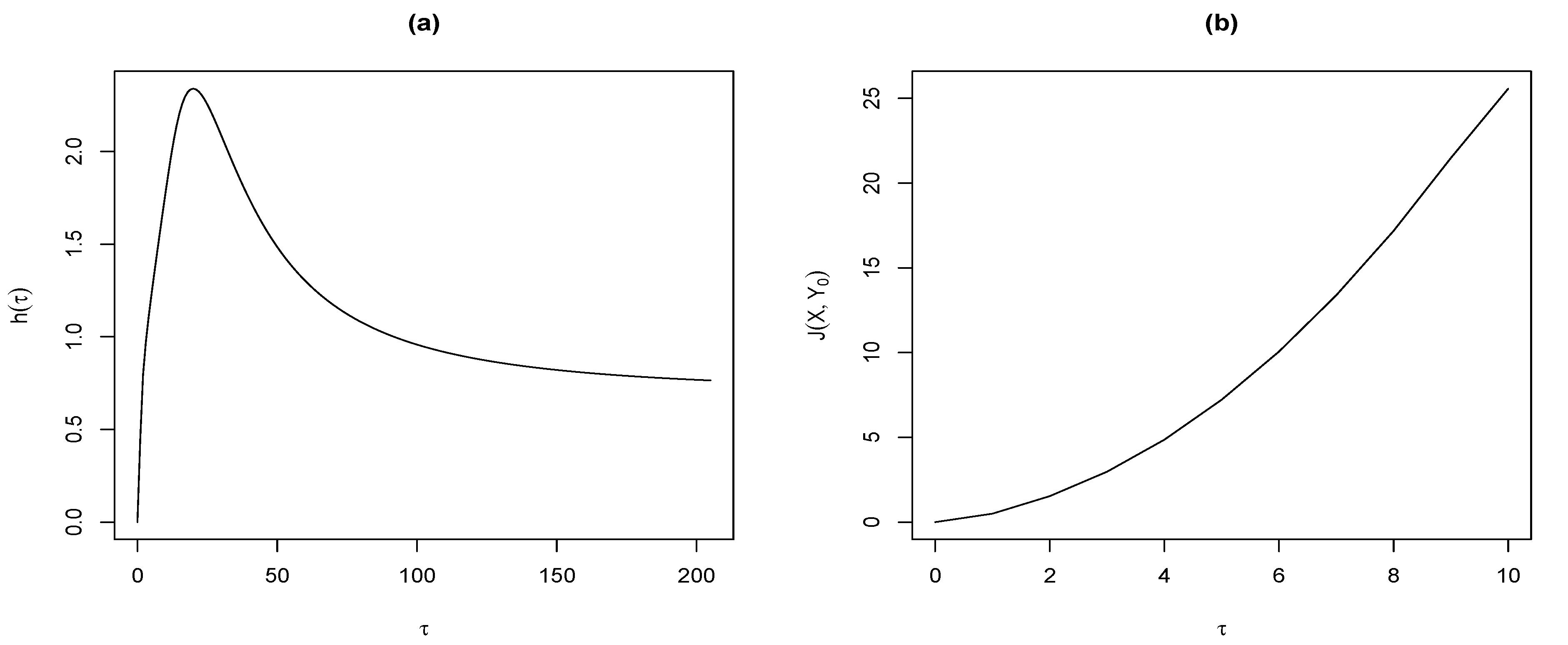
Figure 2 shows in panel (a) several values of $h\left(\tau \right)=E[log\{2\Phi \left(\tau W\right)\left\}\right]$ for $\tau =0,1,...,200$. It is interesting to notice that the maximum value of this expected value is approximately equal to $2.339$. In the panel (b) this figure shows the values of J-divergence between $X\sim S{N}_1(0,{\tau }^2,\tau )$ and $Y_0\sim N(0,{\tau }^2)$ computed in (7) for $\tau =0,1,...,10$.

Figure 2. (a) Behavior of $h\left(\tau \right)=E[log\{2\Phi \left(\tau W\right)\left\}\right]$ for $\tau =0,1,...,200$. (b) Behavior of $J(X,Y_0)$ for $\tau =0,1,...,10$.

Figure 2. (a) Behavior of $h\left(\tau \right)=E[log\{2\Phi \left(\tau W\right)\left\}\right]$ for $\tau =0,1,...,200$. (b) Behavior of $J(X,Y_0)$ for $\tau =0,1,...,10$.

4. Statistical Application

For a statistical application of this paper, we consider the seismic catalogue of the Servicio Sismológico Nacional of Chile (SSN, [28]) analyzed by [22], containing 6,714 aftershocks on a map [32–${40}^{\circ }$S]×[69–$75.5^{\circ }$E] for a period between 27 February 2010 to 13 July 2011. Our main goal is to compare the aftershock distributions of local and moment magnitudes ($M_l$ and $M_w$, respectively) using the KL-divergence and J-divergence between clusters detected by nonparametric clustering (NPC) method developed by [23] (See Figure 3). This method allows the detection of subsets of points forming clusters associated with high density areas which hinge on an estimation of the underlying probability density function via a nonparametric kernel method for each of these clusters. Consequently, this methodology has the advantage of not requiring some subjective choices on input, such as the number of existing clusters. The aftershock clusters analyzed by [22] consider the high density areas with respect to its map positions, i.e., they consider the bi-dimensional distribution of latitude-longitude joint variable to be estimated by the kernel method. For more details about the NPC method, see also [23].

Figure 3. Left: Map of the Chile region analyzed for post-seismicity correlation with clustering events: black (1), red (2), green (3), blue (4), violet (5), yellow (6) and gray (7).

Figure 3. Left: Map of the Chile region analyzed for post-seismicity correlation with clustering events: black (1), red (2), green (3), blue (4), violet (5), yellow (6) and gray (7).

Depending on the case, we consider it pertinent to analyze the measures of J-divergences between a cluster sample fitted by a skew-normal distribution versus the same sample fitted by a normal distribution, where the fits are previously diagnosed by QQ-plots (see e.g., [20]). The MLE’s of the model parameters are obtained by using the sn package developed by [29] and described later in Section 4.1; the entropies, cross-entropies, KL-divergence and J-divergences presented in the previous sections are computed using skewtools package developed by [30]. Both packages are implemented in R software [31]. In Section 4.2 we present the Kupperman test [32] based on asymptotic approximation of the KL-divergence statistic to chi-square distribution with degrees of freedom depending on the dimension of the parametric space.

4.1. Likelihood Function

In order to examine the usefulness of the KL-divergence and J-divergence between multivariate skew-normal distributions developed in this paper, we consider the MLE’s of the location, dispersion and shape/skewness parameters proposed by [17] (and considered for a meteorological application in [20]) for a sample of independent observations ${\mathbf{Z}}_i\sim S{N}_k(\mathbf{\xi },\Omega ,\mathbf{\eta })$, $i=1,...,N$. We estimate the parameters by numerically maximizing the log-likelihood function:

$$logL\left(\mathbf{\theta }\right)\propto -\frac{N}{2}log|\Omega |-\frac{N}{2}\mathrm{tr}\left({\Omega }^{-1}\mathbf{V}\right)+\sum _{i=1}^{N}log[\Phi \left\{{\mathbf{\eta }}^{\top }{\Omega }^{-1/2}({\mathbf{z}}_i-\mathbf{\xi })\right\}],$$

where

$$\mathbf{V}=\frac{1}{N}\sum _{i=1}^N({\mathbf{z}}_i-\mathbf{\xi }){({\mathbf{z}}_i-\mathbf{\xi })}^{\top }$$

and $\mathbf{\theta }=\{\mathbf{\xi },\Omega ,\mathbf{\eta }\}$. Then, we can obtain $\widehat{\mathbf{\theta }}=\{\widehat{\mathbf{\xi }},\widehat{\Omega },\widehat{\mathbf{\eta }}\}=arg{max}_{\mathbf{\theta }}L\left(\mathbf{\theta }\right)$ using the Newton–Rhapson method. This method works well for distributions with a small number of k-variables. Other similar methods such as the EM algorithm tend to have more robust relativity but run slower than MLE.

4.2. Asymptotic Test

Following [32,33], in this section we consider the asymptotic properties of the likelihood estimator of the J-divergence between the distributions of two random vectors $\mathbf{X}$ and $\mathbf{Y}$. For this, it is assumed that $\mathbf{X}$ and $\mathbf{Y}$ have pdf indexed by unknown parameters vectors ${\mathbf{\theta }}_1$ and ${\mathbf{\theta }}_2$, respectively, which belong to the same parameters space. Let ${\widehat{\mathbf{\theta }}}_1={({\widehat{\theta }}_{11},\dots ,{\widehat{\theta }}_{1p})}^{\top }$ and ${\widehat{\mathbf{\theta }}}_2={({\widehat{\theta }}_{21},\dots ,{\widehat{\theta }}_{2p})}^{\top }$ be the MLE’s of the parameter vectors ${\mathbf{\theta }}_1={({\theta }_{11},\dots ,{\theta }_{1p})}^{\top }$ and ${\mathbf{\theta }}_2={({\theta }_{21},\dots ,{\theta }_{2p})}^{\top }$, respectively, based on independent samples of size $N_1$ and $N_2$ from the distributions of $\mathbf{X}$ and $\mathbf{Y}$, respectively. Denote by $J({\mathbf{\theta }}_1,{\mathbf{\theta }}_2)$ the J-divergence between the distributions of $\mathbf{X}$ and $\mathbf{Y}$, and consider the statistic defined by

$$S_{KL}({\widehat{\mathbf{\theta }}}_1,{\widehat{\mathbf{\theta }}}_2)=\frac{N_1{N}_2}{N_1+N_2}J({\widehat{\mathbf{\theta }}}_1,{\widehat{\mathbf{\theta }}}_2).$$

Under the regularity conditions discussed by [33], it follows that if $\frac{N_1}{N_1+N_2}\underset{N_1,N_2\to \infty }{⟶}\lambda$, with $0<\lambda <1$, then under the homogeneity null hypothesis $H_0:{\mathbf{\theta }}_1={\mathbf{\theta }}_2$,

$$\begin{array}{c}\hfill S_{\mathrm{KL}}({\widehat{\mathbf{\theta }}}_1,{\widehat{\mathbf{\theta }}}_2)\underset{N_1,N_2\to \infty }{\stackrel{d}{⟶}}{\chi }_p^2\end{array}$$

(10)

where “$\stackrel{d}{⟶}$" means convergence in distribution.

Based on (10) an asymptotic statistical hypothesis tests for the null hypothesis $H_0:{\mathbf{\theta }}_1={\mathbf{\theta }}_2$ can be derived. Consequently, it can be implemented in terms of the J-divergence (or the KL-divergence, as in [3]) between the multivariate skew-normal distributions $\mathbf{X}\sim S{N}_k({\mathbf{\xi }}_1,{\Omega }_1,{\mathbf{\eta }}_1)$ and $\mathbf{Y}\sim S{N}_k({\mathbf{\xi }}_2,{\Omega }_2,{\mathbf{\eta }}_2)$, for which ${\mathbf{\theta }}_1$ and ${\mathbf{\theta }}_2$ are the corresponding $p=2k+k(k+1)/2$ different unknown parameters in $\{{\mathbf{\xi }}_1,{\Omega }_1,{\mathbf{\eta }}_1\}$ and $\{{\mathbf{\xi }}_2,{\Omega }_2,{\mathbf{\eta }}_2\}$, respectively. Hence, (10) allows testing through the P-value if the homogeneity null hypothesis $H_0:{\mathbf{\xi }}_1={\mathbf{\xi }}_2,{\Omega }_1={\Omega }_2,{\mathbf{\eta }}_1={\mathbf{\eta }}_2$ is rejected or not. Thus, if for large values of $N_1$, $N_2$ we observe $S_{\mathrm{KL}}({\widehat{\mathbf{\theta }}}_1,{\widehat{\mathbf{\theta }}}_2)=s$, then the homogeneity null hypothesis can be rejected at level α if $P({\chi }_p^2>s)\le \alpha$.

4.3. Main Results

The skew-normal KL-divergence values of Proposition 1 for each pair of clusters are reported in Table 1. By (4), we can obtain the symmetrical skew-normal J-divergences to compare the parametric differences between these clusters. The MLE’s of the unknown parameters for the distribution of each cluster are shown in Table 2 with its respective descriptive statistics and estimated skew-normal model parameters. 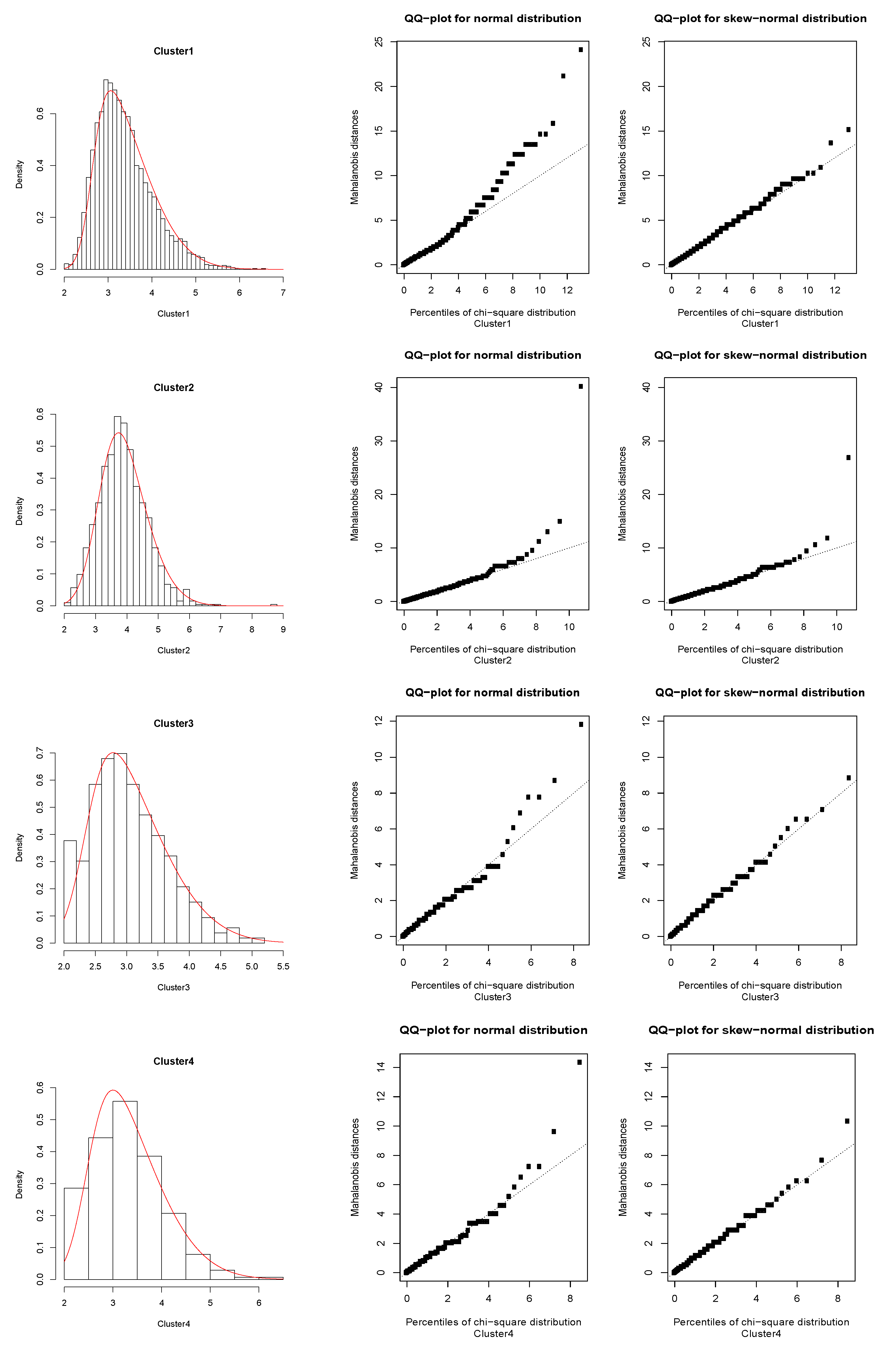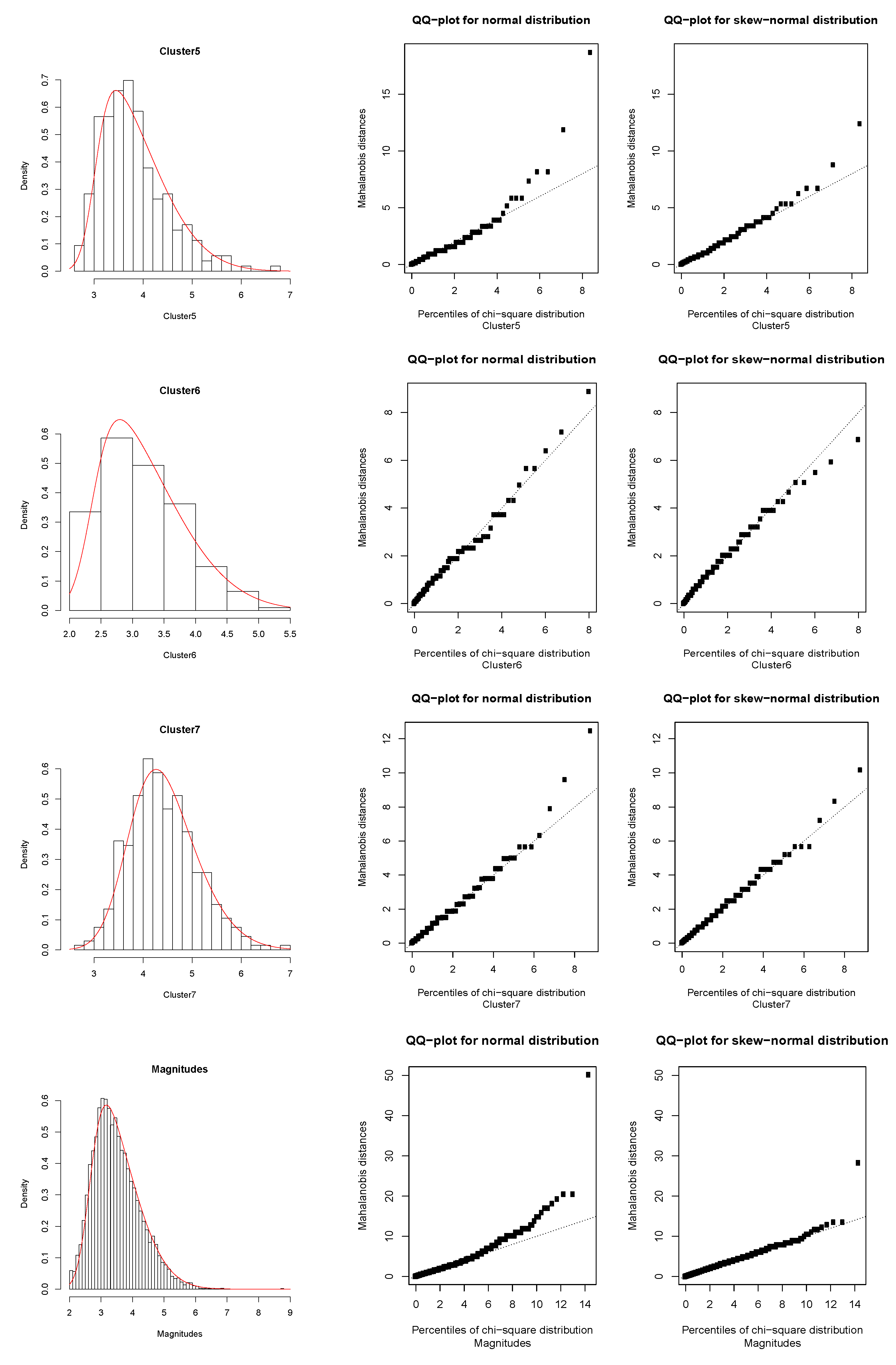In the Appendix B, we attach the Figure A1 and Figure A2 which indicate the performance of the fitted models, where we also include the QQ-plots for the normal and skew-normal cases. These QQ-plots represent the dispersion of the Mahalanobis distances related to the theoretical parameters, with respect to the empirical percentiles of the chi-square distribution. It follows from there that as the dispersion line is fitted by the theoretical line in a greater degree, the skew-normal fit will have better performance. The diagnostic QQ-plots are also possible to obtain by using the sn package developed by [29].

Table 1. KL-divergences for pairs of clusters.

Cluster	black (1)	red (2)	green (3)	blue (4)	violet (5)	yellow (6)	gray (7)
black (1)	0	0.178	0.149	0.008	0.262	0.041	0.835
red (2)	0.219	0	0.743	0.267	0.018	0.455	0.273
green (3)	0.181	0.601	0	0.102	0.909	0.038	1.688
blue (4)	0.015	0.234	0.095	0	0.374	0.015	0.981
violet (5)	0.212	0.018	0.721	0.269	0	0.437	0.216
yellow (6)	0.053	0.350	0.031	0.020	0.530	0	1.194
gray (7)	0.978	0.224	1.887	1.032	0.274	1.398	0

Table 1. KL-divergences for pairs of clusters.

Cluster	black (1)	red (2)	green (3)	blue (4)	violet (5)	yellow (6)	gray (7)
black (1)	0	0.178	0.149	0.008	0.262	0.041	0.835
red (2)	0.219	0	0.743	0.267	0.018	0.455	0.273
green (3)	0.181	0.601	0	0.102	0.909	0.038	1.688
blue (4)	0.015	0.234	0.095	0	0.374	0.015	0.981
violet (5)	0.212	0.018	0.721	0.269	0	0.437	0.216
yellow (6)	0.053	0.350	0.031	0.020	0.530	0	1.194
gray (7)	0.978	0.224	1.887	1.032	0.274	1.398	0

We can see from Table 1 that the grey (7) cluster has the larger discrepancy with respect to the other clusters, except with respect to red (2) and violet (5) clusters, which is mainly due to the location and shape fitted parameters (see Table 2). A counterpart case is found for the green (3) cluster, which presents greater differences with respect to these two aforementioned clusters. On the other hand, the diagnostic QQ-plots show good performance of the skew-normal fit with respect to the normal case, although we should observe here that the red (2) cluster is being affected by an outlier observation corresponding to the greater magnitude $M_w=8.8$. However, this fit considers that the probability of a similar occurrence in the future of a great event like this is practically zero.

Given that the seismic observations have been classified by the NPC method considering their positions on the map, the KL-divergence and J-divergence based on magnitudes proposed in this paper are not valid tools to corroborate the clustering method. Nevertheless, these measures corroborate some similarities in the distributions of those clusters localized away from the epicenter as, e.g., red (2)–violet (5) and green (3)–yellow (6), as well as some discrepancies in the distributions of some clusters as, e.g., red (2)–green (3), red (2)–blue (4) and gray (7)–black (1). All of these similarities and discrepancies were evaluated through the Kupperman test (10). Table 3 reports the statistic test values and the corresponding P-values obtained by comparing the asymptotic reference chi-square distribution with $p=3$ degrees of freedom ($k=1$). We can see that this test corroborates the similarities in the distribution of the clusters red (2)–violet (5) and green (3)–yellow (6), but this test also suggests similarities for the black (1)–blue (4) and blue (4)–yellow (6) clusters. These results are consistent with the values of the fitted parameters, as we can see in Table 2. In this last table we have also presented the values of the parameter $\tau ={({\eta }^2\Omega )}^{1/2}$ for each cluster and the divergence $J(X,Y_0)$ between skew-normal and normal distributions defined in Equation (7). Specifically, since the shape/skewness parameters of red (2) and gray (7) clusters are the smallest, it is then evident that the lower values for the divergence $J(X,Y_0)$ correspond to these clusters, a result that is consistent with the panel (b) Figure 2.

Table 2. Mean and standard deviation (sd) from the normal fit, minimum (min), maximum (max) and number of observations (N) for each cluster and for the full data (see “Total” below); skew-normal MLE’s and their respective standard deviations (in brackets) for each and the full cluster; τ and $J(X,Y_0)$ values for each and the full cluster.

Cluster		Descriptive Statistics						Skew-normal fit
		mean	sd	min	max	N		ξ	Ω	η		τ	$J(X,Y_0)$
black (1)		3.427	0.655	2.0	6.6	4182		3.430 (0.010)	0.651 (0.008)	0.756 (0.020)		0.610	0.211
red (2)		3.924	0.769	2.1	8.8	962		3.927 (0.025)	0.766 (0.019)	0.445 (0.068)		0.389	0.092
green (3)		3.085	0.615	2.0	5.2	265		3.081 (0.038)	0.618 (0.030)	0.711 (0.105)		0.559	0.181
blue (4)		3.339	0.729	2.0	6.1	280		3.337 (0.043)	0.730 (0.035)	0.697 (0.101)		0.595	0.202
violet (5)		3.852	0.682	2.6	6.8	265		3.858 (0.041)	0.673 (0.033)	0.820 (0.067)		0.673	0.252
yellow (6)		3.215	0.666	2.1	5.2	215		3.201 (0.047)	0.683 (0.040)	0.805 (0.128)		0.665	0.247
gray (7)		4.447	0.695	2.7	6.9	332		4.447 (0.038)	0.694 (0.029)	0.453 (0.124)		0.378	0.087
Total		3.539	0.743	2.0	8.8	6584		3.539 (0.009)	0.743 (0.007)	0.731 (0.018)		0.629	0.224

Table 2. Mean and standard deviation (sd) from the normal fit, minimum (min), maximum (max) and number of observations (N) for each cluster and for the full data (see “Total” below); skew-normal MLE’s and their respective standard deviations (in brackets) for each and the full cluster; τ and $J(X,Y_0)$ values for each and the full cluster.

Cluster		Descriptive Statistics						Skew-normal fit
		mean	sd	min	max	N		ξ	Ω	η		τ	$J(X,Y_0)$
black (1)		3.427	0.655	2.0	6.6	4182		3.430 (0.010)	0.651 (0.008)	0.756 (0.020)		0.610	0.211
red (2)		3.924	0.769	2.1	8.8	962		3.927 (0.025)	0.766 (0.019)	0.445 (0.068)		0.389	0.092
green (3)		3.085	0.615	2.0	5.2	265		3.081 (0.038)	0.618 (0.030)	0.711 (0.105)		0.559	0.181
blue (4)		3.339	0.729	2.0	6.1	280		3.337 (0.043)	0.730 (0.035)	0.697 (0.101)		0.595	0.202
violet (5)		3.852	0.682	2.6	6.8	265		3.858 (0.041)	0.673 (0.033)	0.820 (0.067)		0.673	0.252
yellow (6)		3.215	0.666	2.1	5.2	215		3.201 (0.047)	0.683 (0.040)	0.805 (0.128)		0.665	0.247
gray (7)		4.447	0.695	2.7	6.9	332		4.447 (0.038)	0.694 (0.029)	0.453 (0.124)		0.378	0.087
Total		3.539	0.743	2.0	8.8	6584		3.539 (0.009)	0.743 (0.007)	0.731 (0.018)		0.629	0.224

Table 3. J-divergences for each pair of clusters. The statistic values and P-values of the asymptotic test are given in brackets. Those marked in bold correspond to the P-values higher than a probability 0.04 related to a 4% significance level.

Cluster	black (1)	red (2)	green (3)	blue (4)	violet (5)	yellow (6)	gray (7)
black (1)	0	0.397	0.330	0.023	0.475	0.093	1.814
	(0; 1)	(311; 0)	(82; 0)	(6.1; 0.106)	(118; 0)	(19; 0)	(558; 0)
red (2)	0.397	0	1.344	0.501	0.037	0.805	0.497
	(311; 0)	(0; 1)	(279; 0)	(109; 0)	(7.6; 0.055)	(142; 0)	(123; 0)
green (3)	0.330	1.344	0	0.197	1.630	0.069	3.575
	(82; 0)	(279; 0)	(0; 1)	(27; 0)	(216; 0)	(8.1; 0.043)	(527; 0)
blue (4)	0.023	0.501	0.197	0	0.642	0.035	2.014
	(6.1; 0.106)	(109; 0)	(27; 0)	(0; 1)	(88; 0)	(4.2; 0.239)	(306; 0)
violet (5)	0.475	0.037	1.630	0.642	0	0.967	0.490
	(118; 0)	(7.6; 0.055)	(216; 0)	(88; 0)	(0; 1)	(115; 0)	(72; 0)
yellow (6)	0.093	0.805	0.069	0.035	0.967	0	2.593
	(19; 0)	(142; 0)	(8.1; 0.043)	(4.2; 0.239)	(115; 0)	(0; 1)	(338; 0)
gray (7)	1.814	0.497	3.575	2.014	0.490	2.593	0
	(558; 0)	(123; 0)	(527; 0)	(306; 0)	(72; 0)	(338; 0)	(0; 1)

Table 3. J-divergences for each pair of clusters. The statistic values and P-values of the asymptotic test are given in brackets. Those marked in bold correspond to the P-values higher than a probability 0.04 related to a 4% significance level.

Cluster	black (1)	red (2)	green (3)	blue (4)	violet (5)	yellow (6)	gray (7)
black (1)	0	0.397	0.330	0.023	0.475	0.093	1.814
	(0; 1)	(311; 0)	(82; 0)	(6.1; 0.106)	(118; 0)	(19; 0)	(558; 0)
red (2)	0.397	0	1.344	0.501	0.037	0.805	0.497
	(311; 0)	(0; 1)	(279; 0)	(109; 0)	(7.6; 0.055)	(142; 0)	(123; 0)
green (3)	0.330	1.344	0	0.197	1.630	0.069	3.575
	(82; 0)	(279; 0)	(0; 1)	(27; 0)	(216; 0)	(8.1; 0.043)	(527; 0)
blue (4)	0.023	0.501	0.197	0	0.642	0.035	2.014
	(6.1; 0.106)	(109; 0)	(27; 0)	(0; 1)	(88; 0)	(4.2; 0.239)	(306; 0)
violet (5)	0.475	0.037	1.630	0.642	0	0.967	0.490
	(118; 0)	(7.6; 0.055)	(216; 0)	(88; 0)	(0; 1)	(115; 0)	(72; 0)
yellow (6)	0.093	0.805	0.069	0.035	0.967	0	2.593
	(19; 0)	(142; 0)	(8.1; 0.043)	(4.2; 0.239)	(115; 0)	(0; 1)	(338; 0)
gray (7)	1.814	0.497	3.575	2.014	0.490	2.593	0
	(558; 0)	(123; 0)	(527; 0)	(306; 0)	(72; 0)	(338; 0)	(0; 1)

5. Conclusions

We have presented a methodology to compute the Kullback–Leibler divergence for multivariate data presenting skewness, specifically, for data following a multivariate skew-normal distribution. The calculation of this measure is semi-analytical, since it is the sum of two analytical terms, one corresponding to the multivariate normal Kullback–Leibler divergence and the other depending on the location, dispersion and shape parameters, and a third term which must be computed numerically and which was reduced from a multidimensional integral to an integral in only one dimension. Numerical experiments have shown that the performance of this measure is consistent with its theoretical properties. Additionally, we have derived expressions for the J-divergence between different multivariate skew-normal distributions, and in particular for the J-divergence between the skew-normal and normal distributions. The presented entropy and KL-divergence concepts for this class of distributions are necessary to compute other information tools as mutual information.

This work has also presented a statistical application related to aftershocks produced by the Maule earthquake which occurred on 27 February 2010. The results shown that the proposed measures are useful tools for comparing the distributions of magnitudes of events related to the regions near the epicenter. We also consider an asymptotic homogeneity test for the cluster distributions under the skew-normality assumption and, consequently, confirm the found results in a consistent form.