Function Based Fault Detection for Uncertain Multivariate Nonlinear Non-Gaussian Stochastic Systems Using Entropy Optimization Principle

Abstract

In this paper, the fault detection in uncertain multivariate nonlinear non-Gaussian stochastic systems is further investigated. Entropy is introduced to characterize the stochastic behavior of the detection errors, and the entropy optimization principle is established for the fault detection problem. The principle is to maximize the entropies of the stochastic detection errors in the presence of faults and to minimize the entropies of the detection errors in the presence of disturbances. In order to calculate the entropies, the formulations of the joint probability density functions (JPDFs) of the stochastic errors are presented in terms of the known JPDFs of both the disturbances and the faults. By using the novel performance indexes and the formulations for the entropies of the detection errors, new fault detection design methods are provided for the considered multivariate nonlinear non-Gaussian plants. Finally, a simulation example is given to illustrate the efficiency of the proposed fault detection algorithm.

1. Introduction

Fault detection (FD) has long been regarded as an important and integrated part in modern control systems for improving reliability [1,2,3,4,5,6,7,8,9,10]. The so-far obtained approaches include the system identification technique [2] and the statistic approaches based on the Bayesian theorem, likelihood methods and hypothesis test techniques [11]. Besides, filters or observers have been widely used to generate the residual signal for fault detection and estimation [2,6,8,9,12,13,14,15,16,17,18,19,20].

Among the above results, for dynamic stochastic systems, the filter-based approach has been shown as an effective way where generally the noises or disturbances are supposed to be Gaussian [21,22] and the filter design objective is to realize a minimum variance residual. However, in many chemical and manufacturing processes, the inputs involved are non-Gaussian[19,20,23,24,25,26]. For example, in paper making, the length of fibre and the size of filling molecular weight are important input variables, but none of them would obey a Gaussian distribution. This is simply because most random variables and random processes are bounded in paper web formation system. Actually, even for stochastic systems with Gaussian inputs, nonlinearities in the system may lead to non-Gaussian outputs. For the non-Gaussian variables (vectors), it is well-known that the expectation and variance are insufficient to characterize their statistics. As a result, new measures should be adopted. Entropy is a known measure that describes the average information contained in the given PDF (JPDF), which has been widely used in information, thermodynamics and control fields [6,8,27,28,29,30]. By minimizing the entropy, higher order moments can be minimized with respect to the random variables [13,26,27,31,32,33].

Nevertheless, since entropy is an integral operation of PDF while a PDF is a non-linear function with an integral constraint and a positive constraint, it is not easy to find the dynamical relationships between the PDFs of the input and the concerned output and further to formulate the entropies of the distribution of outputs. Besides, for random vectors, the formulation for the JPDF of the output becomes much more complicated than the case of random variables even if the transform matrix is linear. For example, in [6], ${\pi }_{k+1}\in {[a,b]}^n$ is supposed to be a non-Gaussian continuous random vector, $D_k\in R^{m\times n},$ after the multivariate mapping ${\theta }_{k+1}=D_k{\pi }_{k+1},$ the JPDF of ${\theta }_{k+1}$ should be discussed for three different cases based on $D_k$ and ${\theta }_{k+1}$ is not continuous any more except that $D_k$ is invertible. Thus, the existing concept of entropy has to be extended. In fact, the approach presented in [6] holds only for linear systems with special form of system matrices when applied to FD.

In this paper, the filter-based FD approach for uncertain multivariate nonlinear non-Gaussian stochastic system is further investigated using the entropy optimization principle. Firstly, a novel filtering and filter-based FD framework is established to construct a residual such that the fault can be detected from the changes of the residual. Secondly, the formulations between the JPDFs of the disturbances and faults and those of the detection errors are established. The entropy optimization principles are then presented to calculate the gain matrix of the optimal FD filter.

The remainder of this paper is organized as follows. Section 2 presents the preliminaries. In Section 2.1 and Section 2.2, the nonlinear difference model and the corresponding filter model are described. In Section 2.3, the definition of entropy is introduced for the detection errors and the basic relationships are formulated between the entropy of the input and the output. The main results are given in Section 3, where the entropy optimization performance index is proposed in Section 3.1 and its corresponding formulations for entropies are established in Section 3.2. In order to calculate the JPDFs of the detection errors, the simplified algorithms are provided in Section 3.3 and the FD filtering algorithms are finally given in Section 3.4 to compute the optimal FD filter gain using the proposed entropy optimization principle. A simple simulation example is provided in Section 4 to demonstrate the effectiveness of the main results. Conclusion is given in Section 5.

In the following, unless stated otherwise, matrices are assumed to have compatible dimensions. The identity and zero matrices are denoted by I and 0 respectively with appropriate dimensions. For a square matrix M, its inverse and determinant are denoted by $M^{-1}$ and $detM$ respectively. For two real vectors $v_1$ and $v_2$, the notation $v_1⪰v_2$ means that every element of $v_1$ is no less than the corresponding one of $v_2$ and $\parallel v_1{\parallel }_2$ is used to denote the Euclidean norm. For a multivariate nonlinear smooth function $y=g\left(x\right)$, $\frac{\partial g\left(x\right)}{\partial x}$ denotes its Jacobian matrix. For a random vector $z,$ the formula $P\{z⪯\tau \}$ represents the joint probability of event $z⪯\tau$, $F_z(·)$ denotes its joint probability distribution function, ${\gamma }_z(·)$ denotes the corresponding joint probability density function (JPDF), and $H\left(z\right),\epsilon \left(z\right)$ are used to denote its entropy and expectation, respectively.

2. Preliminary

2.1. Plant Models

Consider a multivariate nonlinear stochastic discrete-time system described by

$$\left\{\begin{array}{c}{x}_{k+1}=F_0(x_k,{\delta }_k,w_k)+▵F\hfill \\ y_k=G(x_k,v_k)\hfill \end{array}\right.$$

(1)

where $x_k\in R^n$ is the state, $y_k\in R^m$ is the output, $w_k\in R^p$ is the stochastic disturbance input, $v_k\in R^m$ is the disturbance influencing on the output and ${\delta }_k\in R^q$ is the fault to be detected. $F_0(.,.,.)$ is a known multivariate Borel measurable and smooth nonlinear functions of their arguments, $▵F$ represents the uncertainty satisfying ${\parallel ▵F\parallel }_2\le {\delta }_0$ and $|det\frac{\partial F_0(.,.,.)}{\partial w_k}|\ne 0$ holds for any $w_k\in {[a,b]}^p$.

It should be pointed out that ${\delta }_k$, $w_k$ and $v_k$ are supposed to be arbitrary bounded independent random vectors rather than Gaussian ones, which is different from the existing FD approaches based on the Kalman filtering theory. It is noted that ${\delta }_k$ can also represent the abrupt change of the model parameters. This model is actually a generalization of those where only additive faults or unexpected changes of model parameters are concerned.

To simplify the FD design procedures, the following assumptions are required, which can be satisfied by many practical processes.

Assumption 1. $x_0$, ${\delta }_k$, $v_k$ and $w_k$ $(k=0,1,2,\cdots )$ are bounded, mutually independent random vectors with known JPDFs denoted as ${\gamma }_{x_0}\left(\tau \right)$, ${\gamma }_{\delta }\left(\tau \right)$, ${\gamma }_v\left(\tau \right)$ and ${\gamma }_w\left(\tau \right),$ respectively. ${\gamma }_w\left(\tau \right)={\gamma }_{w_0}\left(\tau \right)+▵{\gamma }_w\left(\tau \right)$ where ${\gamma }_{w_0}\left(\tau \right)$ is a known function defined on ${[a,b]}^p$ and $▵{\gamma }_w\left(\tau \right)$ satisfies $\parallel ▵{\gamma }_w{\left(\tau \right)\parallel }_2\le {\delta }_1.$

Generally speaking, two groups of approaches can be used to determine ${\gamma }_{x_0}\left(\tau \right)$, ${\gamma }_{\delta }\left(\tau \right)$, ${\gamma }_v\left(\tau \right),$ and ${\gamma }_w\left(\tau \right)$. One is the direct measurement using some advanced instruments such as the digital camera. For example, with the developments in image processing, several digital cameras have been used to measure the distribution of the flame in the flame combustion system, which can be further transformed into the temperature distribution. The other is the kernel estimation technique based on the open loop test [34]. In some practical processes (e.g., paper web formation control and particle size distribution control), enormous data can be stored and used to analyze the model of both the disturbances and the faults, with which some probabilistic properties can also be obtained, where the involved random vectors (including both the disturbances and the faults) may also obey the non-Gaussian statistic behaviour [14,15,18,32,35].

Assumption 2. $F_0(·,·,·)$ is a known multivariate $Borel$ measurable and smooth nonlinear functions of their arguments, where $F_0(0,0,0)=0$ holds.

Assumption 3. $G(·,·)=C_k{x}_k+D_k{v}_k$, where $C_k\in R^{m\times n}$ and $m\le n$ hold. Further, $C_k$ is with a full row rank at every sample time, and its first m columns also have full rank (otherwise, the column can be re-arranged to guarantee this assumption). $D_k\in R^{m\times m}$ is an invertible matrix.

2.2. Filter and Error Dynamics

For the nonlinear dynamic system given by (1), the filter can be described by

$$\left\{\begin{array}{c}{\widehat{x}}_{k+1}=F_0({\widehat{x}}_k,0,0)+U_k(y_k-{\widehat{y}}_k)\hfill \\ {\widehat{y}}_k=C_k{\widehat{x}}_k\hfill \end{array}\right.$$

(2)

where $U_k\in R^{n\times m}$ is the filter matrix gain to be determined. Combining (1) with (2), the resulting estimation error $e_k=x_k-{\widehat{x}}_k$ satisfies

$$\begin{array}{ccc}\hfill e_{k+1}& =& \Phi (x_k,{\delta }_k,w_k)\hfill \end{array}$$

(3)

$$\begin{array}{ccc}& =& F_0(x_k,{\delta }_k,w_k)+▵F-U_k{y}_k-F_0({\widehat{x}}_k,0,0)+U_k{\widehat{y}}_k\hfill \end{array}$$

(4)

The residual signal for the fault detection is therefore defined by

$${\widehat{e}}_k=y_k-{\widehat{y}}_k=C_k{e}_k+D_k{v}_k$$

(5)

Related to (4), the vector denoted by

$${\theta }_k=-U_k{y}_k-F_0({\widehat{x}}_k,0,0)+U_k{\widehat{y}}_k$$

(6)

can be regarded as a deterministic term with an unknown matrix gain $U_k.$ The main difficulty is that the term $F_0(x_k,{\delta }_k,w_k)$ in (4) is both nonlinear and multivariate at each sample time. As the detection error, it is supposed that ${\widehat{e}}_k$ is defined on ${[\alpha ,\beta ]}^m,$ where α and β can also be respectively chosen as $-\infty$ and $+\infty$. In the following, we will establish the relationships recursively between the JPDFs of $x_0$, ${\delta }_k$, $v_k$ and $w_k$ with ${\widehat{e}}_k$.

Remark 1. In [8], $e_k$ is considered instead of ${\widehat{e}}_k$ for simplicity based on a rigorous assumption, which may lead to considerable conservations. As such, in this note, ${\widehat{e}}_k$ will be concerned directly for which ${\widehat{e}}_k$ should be affected primarily by the fault ${\delta }_k$ and minimally by the disturbances $v_k$ and $w_k.$

2.3. Entropy and Its Formulation

$H\left(z\right)$ can be regarded as a measure of randomness of z, which is defined as follows.

Definition 1. The entropy for a continuous random vector z is defined by

$$H\left(z\right)=\left\{\begin{array}{cc}-{\int }_{{[\alpha ,\beta ]}^l}{\gamma }_z\left(\tau \right)ln\left({\gamma }_z\left(\tau \right)\right)d\tau \hfill & {\gamma }_z\left(\tau \right)>0\hfill \\ 0\hfill & {\gamma }_z\left(\tau \right)=0\hfill \end{array}\right.$$

(7)

where ${\gamma }_z\left(\tau \right)$ is denoted as the JPDF of z, $z\in {[\alpha ,\beta ]}^l$.

Based on Remark 1, the main task for fault detection is to find $U_k$ such that $H\left({\widehat{e}}_k\right)$ can be influenced by ${\delta }_k$ maximally and by $w_k$ or $v_k$ minimally.

It can be shown that $H\left({\widehat{e}}_k\right),$ as the conditional entropies of $x_{k-1},{\delta }_k$, $v_k$, $w_k$, $▵F$ and $U_k,$ is actually a functional of ${\gamma }_{\delta }\left(\tau \right),$ ${\gamma }_v\left(\tau \right)$, ${\gamma }_w\left(\tau \right)$ and ${\gamma }_{x_{k-1}}\left(\tau \right)$ as well as the underdetermined gain $U_k$, which can be further represented by $H({\widehat{e}}_k\mid x_{k-1},{\delta }_k,w_k,v_k,▵F,U_k)$. In order to calculate the entropies, the JPDFs of the errors have to be formulated in advance. The following result reveals the relationship between the JPDFs of the input and output, subject to a multivariate nonlinear mapping.

Lemma 1. For a multivariate $Borel$ smooth function $\phi =\Gamma \left(\sigma \right)$, if σ is a random vector with known JPDF ${\gamma }_{\sigma }\left(\tau \right)$, the JPDFs of φ can be given by

$${\gamma }_{\phi }\left(\tau \right)=\frac{d\left[{\int }_{{\Omega }_k\left(\tau \right)}{\gamma }_{{\sigma }_k}\left(\rho \right)d\rho \right]}{d\rho }$$

(8)

where for a given $\tau ,$ ${\Omega }_k\left(\tau \right)$ is the definition domain of the random vector σ with ${\Omega }_k\left(\tau \right)=\{\rho \mid \Gamma \left(\rho \right)⪯\tau \}.$

Proof: For a given τ, ${\Omega }_k\left(\tau \right)$ is the set consisting of all events ρ such that $\Gamma \left(\rho \right)⪯\tau$. For the concerned function, φ is also a random vector. Based on Probability theory [27], the joint distribution function of φ can be given by

$$F_{\phi }\left(\tau \right)=P\{\phi ⪯\tau \}={\int }_{{\Omega }_k\left(\tau \right)}{\gamma }_{{\sigma }_k}\left(\rho \right)d\rho$$

(9)

Hence, Equation (8) can be obtained by taking derivatives on both sides of (9).      Q.E.D

The next step is to consider the special relationship between ${\widehat{e}}_k$ and the terms $e_k$, $v_k$ in (5), which is related to the linear mapping $\phi =\Theta \sigma$, where $\Theta \in R^{m\times n}$ is a compatible real matrix.

In the following, Lemma 2 and Lemma 3 will be given respectively according to whether the concerned matrix Θ is invertible.

Lemma 2. If $m=n$ and Θ is invertible, the following relationship holds

$${\gamma }_{\phi }\left(\tau \right)={\gamma }_{\sigma }\left({\Theta }^{-1}\tau \right)\left|det{\Theta }^{-1}\right|$$

(10)

Proof: If Θ is invertible, it can be verified that for given τ, there exists ${\tau }_0$ such that ${\tau }_0={\Theta }^{-1}\tau$. Thus, by using Lemma 1, we have

$${\gamma }_{\phi }\left(\tau \right)d\tau =P\{\tau \prec \phi ⪯\tau +d\tau \}=P\{{\tau }_0\prec \sigma ⪯{\tau }_0+d{\tau }_0\}={\gamma }_{\sigma }\left({\tau }_0\right)d{\tau }_0={\gamma }_{\sigma }\left({\Theta }^{-1}\tau \right)\left|det{\Theta }^{-1}\right|d\tau$$

This process also can be regarded as a generalization of the classical relationship for random variables (see, e.g., Chapter 6, [27]).               Q.E.D

In the other case, Θ is a singular matrix. Corresponding to the structure of $C_k$, supposing Θ is with a full row rank. In this case, there exist a low-triangle invertible matrix $T_1$ and an upper-triangle invertible matrix $T_2$ such that

$$T_1\Theta T_2=\left[\begin{array}{cc}{I}_m\hfill & 0\hfill \end{array}\right]$$

(11)

where $I_m$ represents an $m-$dimensional identical matrix and $T_2$ is invertible with positive diagonal elements.

To simplify the presentation, we denote

$$\tilde{\phi }:=\left[\begin{array}{c}{\tilde{\phi }}^{\left(1\right)}\\ {\tilde{\phi }}^{\left(2\right)}\end{array}\right]=T_1\phi ,\tilde{\sigma }:=T_2^{-1}\sigma =\left[\begin{array}{c}{\tilde{\sigma }}^{\left(1\right)}\\ {\tilde{\sigma }}^{\left(2\right)}\end{array}\right],\tilde{\tau }:=T_1\tau =\left[\begin{array}{c}{\tilde{\tau }}^{\left(1\right)}\\ {\tilde{\tau }}^{\left(2\right)}\end{array}\right]$$

(12)

with compatible dimensions. This implies

$$\tilde{\phi }=\left[\begin{array}{cc}{I}_m\hfill & 0\hfill \end{array}\right]\tilde{\sigma }={\sigma }^{\left(1\right)}$$

(13)

Lemma 3. If $\Theta \in R^{m\times n}$ is with full row rank and $m<n$, then for the linear mapping $\phi =\Theta \sigma$, the following relationship holds

$${\gamma }_{\phi }\left(\tau \right)={\int }_{{[a,b]}^{n-m}}{\gamma }_{\sigma }\left(\eta \right)\left|det{T}_1\right|\left|det{T}_2\right|d{\tilde{\tau }}^{\left(2\right)}$$

(14)

with the auxiliary integral argument η being denoted by $\eta :={\left[\begin{array}{cc}{\left(T_2{T}_1\tau \right)}^T\hfill & {\left(T_2{\tilde{\tau }}^{\left(2\right)}\right)}^T\hfill \end{array}\right]}^T$, where $T_1$ and $T_2$ are denoted by (11) and ${\tilde{\tau }}^{\left(2\right)}$ is denoted by (12).

Proof: To complete the required proof, there are three tasks to be achieved: (1) find ${\gamma }_{\tilde{\sigma }}$ in terms of ${\gamma }_{\sigma };$ (2) formulate ${\gamma }_{\tilde{\phi }}$ in terms of ${\gamma }_{\tilde{\sigma }};$ (3) represent ${\gamma }_{\phi }$ in terms of ${\gamma }_{\tilde{\phi }}.$

Based on Lemma 1, task 1 and 3 can be solved as follows. From (12), it can be shown that the JPDFs of $\tilde{\phi }$ and $\tilde{\sigma }$ should satisfy

$${\gamma }_{\phi }\left(\tau \right)={\gamma }_{\tilde{\phi }}\left(T_1\tau \right)\left|det{T}_1\right|,{\gamma }_{\tilde{\sigma }}\left(ϵ\right)={\gamma }_{\sigma }\left(T_2ϵ\right)\left|det{T}_2\right|$$

(15)

On the other hand, (13) implies that

$$P\left\{\tilde{\phi }⪯{\tilde{\tau }}^{\left(1\right)}\right\}=P\{{\tilde{\sigma }}^{\left(1\right)}⪯{\tilde{\tau }}^{\left(1\right)},{\tilde{\sigma }}^{\left(2\right)}\in {[a,b]}^{n-m}\}$$

(16)

It is noted that both ${\tilde{\tau }}^{\left(1\right)}$ and ${\tilde{\sigma }}^{\left(1\right)}$ are $m-$dimensional sub-vectors as defined by (12). Thus, we have

$$F_{\tilde{\phi }}\left({\tilde{\tau }}^{\left(1\right)}\right)=F_{{\tilde{\sigma }}^{\left(1\right)}}\left({\tilde{\tau }}^{\left(1\right)}\right)={\int }_{{[a,b]}^{n-m}}{F}_{\tilde{\sigma }}\left(\tilde{\tau }\right)d{\tilde{\tau }}^{\left(2\right)}$$

which means that

$$\begin{array}{ccc}\hfill {\gamma }_{\tilde{\phi }}\left({\tilde{\tau }}^{\left(1\right)}\right)& =& \frac{\partial F_{\tilde{\phi }}\left({\tilde{\tau }}^{\left(1\right)}\right)}{\partial {\tilde{\tau }}^{\left(1\right)}}=\frac{\partial F_{{\tilde{\sigma }}^{\left(1\right)}}\left({\tilde{\tau }}^{\left(1\right)}\right)}{\partial {\tilde{\tau }}^{\left(1\right)}}\hfill \end{array}$$

$$\begin{array}{ccc}& =& {\gamma }_{{\tilde{\sigma }}^{\left(1\right)}}\left({\tilde{\tau }}^{\left(1\right)}\right)={\int }_{{[a,b]}^{n-m}}{\gamma }_{\tilde{\sigma }}\left(\tilde{\tau }\right)d{\tilde{\tau }}^{\left(2\right)}\hfill \end{array}$$

(17)

As such, task 2 is completed. Combining (15) with (17) yields (14).       Q.E.D

Remark 2. In Lemma 3, if $m=n$, according to matrix theory, $T_2=T_1^{{}^{\prime }}$ holds. In this case, $\Theta ={\left(T_2{T}_1\right)}^{-1}$ and

$$\begin{array}{ccc}\hfill {\gamma }_{\phi }\left(\tau \right)& =& {\gamma }_{\sigma }\left(\eta \right)\left|det{T}_1\right|\left|det{T}_2\right|\hfill \\ & =& {\gamma }_{\sigma }\left(T_2{T}_1\tau \right)\left|det{T}_2{T}_1\right|\hfill \\ & =& {\gamma }_{\sigma }\left({\Theta }^{-1}\tau \right)\left|det{\Theta }^{-1}\right|\hfill \end{array}$$

which implies that Lemma 3 is consistent with Lemma 2 when both the row rank and the column rank of Θ is m.

3. Main Results

3.1. Performance Indexes

Following the above procedures, the fault detection objective can be performed by judging the changes of ${\widehat{e}}_k$ at every sample time, where the entropies of ${\widehat{e}}_k$ only in the presence of $v_k$ and $w_k$ are minimized, but the entropies resulting from ${\delta }_k$ are maximized. After the corresponding performance indexes are established, the involved filter gain can be designed based on the entropy optimization principle.

Generally speaking, there are two main tasks to finish in the following procedures. The first one is to provide appropriate optimization principles to achieve the FD objectives, which are represented by the entropies of ${\widehat{e}}_k$. The second one is to formulate the entropies and PDFs of ${\widehat{e}}_k$ in terms of the PDFs of $x_0$, $v_k$, $w_k$ and $x_k$, ${\delta }_k$, as well as $\Delta F$ .

In this subsection, we will focus on the entropy optimization principle. The JPDF of ${\widehat{e}}_k$($e_k$) in the presence of $v_k,w_k$ and $\Delta F$ and in the absence of ${\delta }_k$ can be represented by ${\gamma }_{{\widehat{e}}_k}^0$(${\gamma }_{e_k}^0$), while that in the presence of ${\delta }_k,\Delta F$ and in the absence of $v_k,w_k$ can be represented by ${\gamma }_{{\widehat{e}}_k}^1$(${\gamma }_{e_k}^1$). Similarly, we denote $H^0({\widehat{e}}_k\mid x_{k-1},v_k,w_k,U_k,\Delta F)$ ($H^1({\widehat{e}}_k\mid x_{k-1},{\delta }_k,U_k,\Delta F)$) as the entropy of ${\widehat{e}}_k$ in the presence of $v_k,w_k,\Delta F$ and in the absence of ${\delta }_k$ (in the presence of ${\delta }_k,\Delta F$ and in the absence of $v_k,w_k$). Concretely it can be further denoted that for $i=0,1,$

$$H^i\left({\widehat{e}}_k\right)=\left\{\begin{array}{cc}-{\int }_{{[\alpha ,\beta ]}^m}{\gamma }_{{\widehat{e}}_k}^i\left(\tau \right)ln\left({\gamma }_{{\widehat{e}}_k}^i\left(\tau \right)\right)d\tau \hfill & {\gamma }_{{\widehat{e}}_k}^i\left(\tau \right)>0\hfill \\ 0\hfill & {\gamma }_{{\widehat{e}}_k}^i\left(\tau \right)=0\hfill \end{array}\right.$$

(18)

where $H^i\left({\widehat{e}}_k\right)$ ($i=0,1$) represents the conditional entropies $H^0({\widehat{e}}_k\mid x_{k-1},v_k,w_k,U_k,\Delta F)$ and $H^1({\widehat{e}}_k\mid x_{k-1},{\delta }_k,U_k,\Delta F)$ respectively for brevity.

Based on (2), (4), (5) and Assumption 3, it can be claimed that only the first m rows of $U_k$ are related to $H^i\left({\widehat{e}}_{k+1}\right)$ while the last $n-m$ rows are irrelevant to the entropy. This means that in this case, $U_{k,m+1},\cdots ,U_{k,n}$ in (19) are redundant vectors for the optimization, where $U_{k,m+1}=\cdots =U_{k,n}=0$ can be selected under this circumstance.

Since $U_k$ is an $n\times m$ matrix, in order to use conventional optimization techniques, we denote

$$U_k={[U_{k1}^T\cdots U_{kn}^T]}^T,u_k={[U_{k1}\cdots U_{kn}]}^T$$

(19)

where $U_{ki}$ is the row vector of $U_k$ and thus $u_k\in R^{mn\times 1}$ is a stretched column vector.

The entropy optimization performance index is proposed as follows

$$J_N\left({\widehat{e}}_k\right):=\sum _{k=1}^{N}J({\widehat{e}}_k,x_{k-1},{\delta }_k,w_k,v_k,u_k)=\sum _{k=1}^N\left[-H^0\left({\widehat{e}}_k\right)+\frac{1}{2}{u}_k^T{R}_1{u}_k+R_2{H}^1\left({\widehat{e}}_k\right)\right]$$

(20)

where $R_1$ and $R_2$ are pre-specified matrix weight and constant weight respectively.

If there exists a filter such that $J_N\left({\widehat{e}}_k\right)$ is minimized for each sample time $N,$ then it is called as an entropy optimization FD filter.

Remark 3. It is noted that entropy optimization is corresponding to variance optimization for Gaussian signals [32]. For example, the entropy optimization principle for FD problems is in parallel to the main results in [2], where linear Gaussian systems were studied and the minimax technology was applied to the variance of errors.

Remark 4. To enhance the FD filtering performance, the expectation vector $\epsilon \left({\widehat{e}}_k\right)$ can also be included in the cost function described in $J_N\left({\widehat{e}}_k\right)$. We can consider the more general performance indexes than $J_N\left({\widehat{e}}_k\right)$ where the entropies of the error resulting from $x_0$, $v_k$, $w_k$ and ${\delta }_k$ are considered simultaneously. However, noting that there is no added difference between the two performance indexes in optimization context, we will focus on $J_N\left({\widehat{e}}_k\right)$ for the FD problem in the following subsections.

Remark 5. In the entropy optimization performance index, $R_1$ and $R_2$ are two pre-specified weights. $R_1$ corresponds to the energy. If there is no restriction on the energy, $R_1$ can be selected as 0. Generally, the smaller $R_1$ is, the easier the fault can be detected. $R_3$ can also be added as the weight of $H^0\left({\widehat{e}}_k\right)$. In that case $R_2$ and $R_3$ are relative, so we set $R_3=1$ and regulate $R_2$. It is noted that the cumulative performance index is adopted in this paper. If there is no sum operation, the index corresponds to the “greedy” one [36]. However, it is shown that the use of long-range prediction can overcome the problem of stabilizing a non-minimum phase plant with unknown or variable dead-time. As such, in this paper, (20) is employed. Moreover, Entropy optimization is equivalent to the variance optimization for Gaussian signals. It can be verified that the entropy optimization is consistent with the results for linear Gaussian systems.

3.2. Formulations for the Error JPDFs

In this subsection, the formulations for the JPDFs related to the FD performance index will be discussed. The JPDFs ${\gamma }_{e_k}^i$ have to be calculated in order to formulate ${\gamma }_{{\widehat{e}}_k}^i$ based on Lemmas 1–3, and then to provide the representation of $H^i\left({\widehat{e}}_k\right)$ ($i=0,1$).

For a given $\tau \in {[\alpha ,\beta ]}^n$, the domains of definition for several involved functions are defined as follows

$$\begin{array}{ccc}\hfill {\Pi }_k^0& :=& \{({\tau }_1,{\tau }_2)\mid \Phi ({\tau }_1,0,{\tau }_2)⪯\tau \},{\Pi }_k^1:=\{({\tau }_1,{\tau }_2)\mid \Phi ({\tau }_1,{\tau }_2,0)⪯\tau \}\hfill \end{array}$$

(21)

$$\begin{array}{ccc}\hfill {\Xi }_k^0& :=& \{({\tau }_1,{\tau }_2)\mid F({\tau }_1,0,{\tau }_2)⪯\tau \},{\Xi }_k^1:=\{({\tau }_1,{\tau }_2)\mid F({\tau }_1,{\tau }_2,0)⪯\tau \}\hfill \end{array}$$

(22)

where the notation ⪯ have been defined in the ending of the Introduction section.

To summarize, the following result can be obtained.

Theorem 1. Under Assumptions 1-3, ${\gamma }_{e_k}^0\left(\tau \right)$ and ${\gamma }_{e_k}^1\left(\tau \right)(k=1,2,\cdots )$ can be calculated from the differentials on the multiple integrations as follows:

$${\gamma }_{e_k}^0\left(\tau \right)=\frac{d\left[\int {\int }_{{\Pi }_k^0\left(\tau \right)}{\gamma }_{x_{k-1},w}({\tau }_1,{\tau }_2)d{\tau }_{1}d{\tau }_2\right]}{d\tau },{\gamma }_{e_k}^1\left(\tau \right)=\frac{d\left[\int {\int }_{{\Pi }_k^1\left(\tau \right)}{\gamma }_{x_{k-1},\delta }({\tau }_1,{\tau }_2)d{\tau }_{1}d{\tau }_2\right]}{d\tau }$$

where

$${\gamma }_{x_k}^0\left(\tau \right)=\frac{d\left[\int {\int }_{{\Xi }_k^0\left(\tau \right)}{\gamma }_{x_{k-1},w}({\tau }_1,{\tau }_2)d{\tau }_{1}d{\tau }_2\right]}{d\tau },{\gamma }_{x_k}^1\left(\tau \right)=\frac{d\left[\int {\int }_{{\Xi }_k^1\left(\tau \right)}{\gamma }_{x_{k-1},\delta }({\tau }_1,{\tau }_2)d{\tau }_{1}d{\tau }_2\right]}{d\tau },$$

and ${\Pi }_k^i\left(\tau \right)$, ${\Xi }_k^i\left(\tau \right)$ ($i=0,1$) are denoted respectively by (21) and (22).

Proof: This result can be obtained similarly to Lemma 1 using the independence property in probability theory.                 Q.E.D

For the FD problem, ${\widehat{e}}_k$ is used as the residual to detect the fault. In order to calculate the entropies of ${\gamma }_{{\widehat{e}}_k}^i\left(\tau \right)$ ($i=0,1$), we denote two auxiliary vectors as follows

$$s_{1k}=C_k{e}_k,s_{2k}=D_k{v}_k$$

and correspondingly to (11), we suppose that there exist $T_{1k}$ and $T_{2k}$ such that

$$T_{1k}{C}_k{T}_{2k}=\left[\begin{array}{cc}{I}_m\hfill & 0\hfill \end{array}\right]$$

Theorem 2. Under Assumptions 1–3, ${\gamma }_{{\widehat{e}}_k}^i\left(\tau \right)$($i=0,1;k=0,1,2,\cdots$) can be calculated from the following

$${\gamma }_{{\widehat{e}}_k}^i\left(\tau \right)={\int }_{{[\alpha ,\beta ]}^m}{\gamma }_{s_{1k}}^i(\tau -{\tau }_1){\gamma }_{s_{2k}}\left({\tau }_1\right)d{\tau }_1$$

where

$${\gamma }_{s_{1k}}^i\left(\tau \right)=\left[{\int }_{{[\alpha ,\beta ]}^{n-m}}{\gamma }_{e_k}^i\left(\eta \right)\left|det{T}_{1k}\right|\left|det{T}_{2k}\right|d{\tilde{\tau }}^{\left(2\right)}\right]$$

and

$${\gamma }_{s_{2k}}\left(\tau \right)={\gamma }_v\left({D_k}^{-1}\tau \right)\left|det{D_k}^{-1}\right|$$

Proof: The formulations of ${\gamma }_{s_{1k}}^i\left(\tau \right)$ can be obtained using Lemma 2 and Lemma 3. Noting ${\widehat{e}}_k=s_{1k}+s_{2k}$, the result can be provided.           Q.E.D

3.3. Simplified Calculation of the Error JPDFs

In the above results, the formulations of the entropies have been reduced to the differentials of some multiple integrals that depend on their integral domains. To simplify the design methods, the following assumption is introduced.

Assumption 4. $det\left[\frac{\partial F(x_k,{\delta }_k,w_k)}{\partial x_k}\right]\ne 0$ holds and $det\left[\frac{\partial \Phi (x_k,{\delta }_k,w_k)}{\partial x_k}\right]\ne 0$ holds for any $x_k$ in their operation domain.

Different from Theorem 1, under Assumption 4, simplified algorithms can be further obtained to calculate ${\gamma }_{e_k}^i\left(\tau \right)$ and then to formulate ${\gamma }_{{\widehat{e}}_k}^i\left(\tau \right)$ ($i=0,1$) by constructing the following auxiliary multivariate functions.

Under Assumption 4, for functions $\Phi (·,·,·)$ and $F(·,·,·)$ and a given vector ${\tau }_1,$ there exist the inverse functions denoted by

$$\delta ={\Phi }^{-1}({\tau }_1,\tau ,0),w={\Phi }^{-1}({\tau }_1,0,\tau )$$

(23)

respectively, which satisfy

$$\tau =\Phi ({\tau }_1,\delta ,0),\tau =\Phi ({\tau }_1,0,w)$$

Construct the auxiliary vectors for ${\gamma }_{e_k+1}$ as

$$\begin{array}{ccc}\hfill {\eta }_{k+1}^0& =& \left[\begin{array}{c}{w}_{k+1}\\ e_{k+1}\end{array}\right],{\Psi }^0(w_{k+1},x_k)=\left[\begin{array}{c}{w}_{k+1}\\ \Phi (x_k,0,w_{k+1})\end{array}\right]\hfill \end{array}$$

(24)

$$\begin{array}{ccc}\hfill {\eta }_{k+1}^1& =& \left[\begin{array}{c}{\delta }_{k+1}\\ e_{k+1}\end{array}\right],{\Psi }^1({\delta }_{k+1},x_k)=\left[\begin{array}{c}{\delta }_{k+1}\\ \Phi (x_k,{\delta }_{k+1},0)\end{array}\right]\hfill \end{array}$$

(25)

And for ${\gamma }_{x_k+1}$, we denote

$$\begin{array}{ccc}\hfill {\xi }_{k+1}^0& =& \left[\begin{array}{c}{w}_{k+1}\\ x_{k+1}\end{array}\right],{{\rm Y}}^0(w_{k+1},x_k)=\left[\begin{array}{c}{w}_{k+1}\\ F(x_k,0,w_{k+1})\end{array}\right]\hfill \end{array}$$

(26)

$$\begin{array}{ccc}\hfill {\xi }_{k+1}^1& =& \left[\begin{array}{c}{\delta }_{k+1}\\ x_{k+1}\end{array}\right],{{\rm Y}}^1({\delta }_{k+1},x_k)=\left[\begin{array}{c}{\delta }_{k+1}\\ F(x_k,{\delta }_{k+1},0)\end{array}\right]\hfill \end{array}$$

(27)

where $\Phi (·,·,·)$ is denoted by (3). With (25) and (24), the dynamics of estimation errors in the presence of ${\delta }_{k+1}$ $\left(w_{k+1}\right)$ and in the absence of $w_{k+1}$ $\left({\delta }_{k+1}\right)$ can also be represented respectively by

$${\eta }_{k+1}^0={\Psi }^0(w_{k+1},x_k),{\eta }_{k+1}^1={\Psi }^1({\delta }_{k+1},x_k),{\xi }_{k+1}^0={{\rm Y}}^0(w_{k+1},x_k),{\xi }_{k+1}^1={{\rm Y}}^1({\delta }_{k+1},x_k)$$

(28)

Using the auxiliary vectors and functions given by (25), (24), (27), (26) and (28), the following results can be obtained.

Theorem 3. Under Assumptions 1–4, ${\gamma }_{e_k}^0\left(\tau \right)$ and ${\gamma }_{e_k}^1\left(\tau \right)$ can be calculated by $(k=0,1,2,\cdots )$

$${\gamma }_{e_{k+1}}^0\left(\tau \right)={\int }_{{[\alpha ,\beta ]}^p}{\gamma }_w\left({\tau }_1\right){\gamma }_{x_k}^0\left({\Phi }^{-1}({\tau }_1,0,\tau )\right){\psi }_0({\tau }_1,\tau )d{\tau }_1$$

(29)

and

$${\gamma }_{e_{k+1}}^1\left(\tau \right)={\int }_{{[\alpha ,\beta ]}^q}{\gamma }_{\delta }\left({\tau }_1\right){\gamma }_{x_k}^1\left({\Phi }^{-1}({\tau }_1,\tau ,0)\right){\psi }_1({\tau }_1,\tau )d{\tau }_1$$

(30)

where

$${\gamma }_{x_{k+1}}^0\left(\tau \right)={\int }_{{[\alpha ,\beta ]}^p}{\gamma }_w\left({\tau }_1\right){\gamma }_{x_k}^0\left(F^{-1}({\tau }_1,0,\tau )\right){\psi }_0({\tau }_1,\tau )d{\tau }_1$$

(31)

$${\gamma }_{x_{k+1}}^1\left(\tau \right)={\int }_{{[\alpha ,\beta ]}^q}{\gamma }_{\delta }\left({\tau }_1\right){\gamma }_{x_k}^1\left(F^{-1}({\tau }_1,\tau ,0)\right){\psi }_1({\tau }_1,\tau )d{\tau }_1$$

(32)

and

$${\psi }_0({\tau }_1,\tau ):={\left|det\frac{\partial F({\tau }_1,0,\tau )}{\partial {\tau }_1}\right|}^{-1},{\psi }_1({\tau }_1,\tau ):={\left|det\frac{\partial F({\tau }_1,\tau ,0)}{\partial {\tau }_1}\right|}^{-1}$$

(33)

Proof: Firstly, from (25) and (28), it can be claimed that ${\gamma }_{e_{k+1}}^1\left(\tau \right)={\int }_{{[\alpha ,\beta ]}^q}{\gamma }_{{\eta }_{k+1}^1}({\tau }_1,\tau )d{\tau }_1$. It is noted that ${\Psi }^1({\delta }_{k+1},x_k)$ is an one-to-one mapping from $({\delta }_{k+1},x_k)$ to $({\delta }_{k+1},e_{k+1})$ under Assumption A.4. Thus, the PDF of $({\delta }_{k+1},e_{k+1})$ can be represented by that of $({\delta }_{k+1},x_k)$ (see e.g., [27]). On the other hand, random vectors $x_k$ and ${\delta }_{k+1}$ can be regarded as mutually independent ones under Assumption A.1. As such, based on the special structure described by (25) and the notations in (23), it can be verified that

$$\begin{array}{ccc}\hfill {\gamma }_{{\eta }_{k+1}^1}({\tau }_1,\tau )& =& {\gamma }_{{\delta }_{k+1}{x}_k}({\tau }_1,\delta ){\left|det\frac{\partial F({\tau }_1,\tau ,0)}{\partial {\tau }_1}\right|}^{-1}={\gamma }_{{\delta }_{k+1}}\left({\tau }_1\right){\gamma }_{x_k}\left({\Phi }^{-1}({\tau }_1,\tau ,0)\right){\left|det\frac{\partial F({\tau }_1,\tau ,0)}{\partial {\tau }_1}\right|}^{-1}\hfill \end{array}$$

$$\begin{array}{ccc}& =& {\gamma }_{{\delta }_{k+1}}\left({\tau }_1\right){\gamma }_{x_k}\left({\Phi }^{-1}({\tau }_1,\tau ,0)\right){\psi }_1({\tau }_1,\tau )\hfill \end{array}$$

(34)

which means that (30) holds. Similarly, by considering the auxiliary vector and function described by ${\eta }_{k+1}^0={\Psi }^0(w_{k+1},x_k)$, we can obtain (32). This procedure can also be used to prove (29) and (31). Q.E.D

With ${\gamma }_{e_k}^i\left(\tau \right)$ ($i=0,1$), ${\gamma }_{{\widehat{e}}_k}^i\left(\tau \right)$ can be obtained by using Theorem 2 so that $H^i\left({\widehat{e}}_k\right)$ can also be formulated for $J_N\left({\widehat{e}}_k\right)$.

3.4. Optimal FD Filter Design Strategy

Based on the above procedures, it can be claimed that the optimization is required for the performance index $J_N\left({\widehat{e}}_k\right)$.

It is noted that (20) leads to

$$J_k\left({\widehat{e}}_k\right)=J_{k-1}\left({\widehat{e}}_k\right)+\left[\Psi \left(u_k\right)+\frac{1}{2}{u}_k^T{R}_1{u}_k\right],k=0,1,2,\cdots ,+\infty$$

(35)

where

$$\Psi \left(u_k\right):=\Psi ({\widehat{e}}_k,u_k)=-H^0\left({\widehat{e}}_k\right)+R_1{H}^1\left({\widehat{e}}_k\right)$$

(36)

The optimal filtering strategy can be obtained through

$$\frac{\partial \left[\Psi ({\widehat{e}}_k,u_k)+\frac{1}{2}{u}_k^T{R}_1{u}_k\right]}{\partial u_k}=0$$

(37)

where an explicit function from other arguments to $u_k$ can be further determined. The principle of optimality can thus result in the optimal FD filtering law for the whole process. To simplify the filter structure, a recursive design procedure is formulated in the following.

Denote

$$u_k=u_{k-1}+\Delta u_k,k=0,1,2,\cdots ,N,\cdots ,+\infty$$

(38)

As a function of $e_k,$ $w_k$ and $\tau ,$ it can be approximated to give

$$\Psi ({\widehat{e}}_k,u_k)={\Psi }_{k0}+{\Psi }_{k1}\Delta u_k+\frac{1}{2}\Delta u_k^T{\Psi }_{k2}\Delta u_k+o(\Delta u_k^T{u}_k)$$

(39)

where

$${\Psi }_{k0}:={\left.{\Psi }_k\left(u_k\right)\right|}_{u_k=u_{k-1}},{\Psi }_{k1}:={\left.\frac{\partial {\Psi }_k\left(u_k\right)}{\partial u_k}\right|}_{u_k=u_{k-1}},{\Psi }_{k2}:={\left.\frac{{\partial }^2{\Psi }_k\left(u_k\right)}{\partial u_k^2}\right|}_{u_k=u_{k-1}}$$

The recursive algorithm can be provided to determine the gain of the entropy optimization FD filter.

Theorem 4. An entropy optimization FD filtering strategy for $J_N$ subject to nonlinear error model (4) is given by

$$\Delta u_k^{*}=-\frac{{\Psi }_{k1}+R_1{u}_{k-1}}{{\Psi }_{k2}+R_1}$$

(40)

for a weight $R_1>0$ satisfying

$${\Psi }_{k2}+R_1>0$$

(41)

Proof: Firstly, it can be seen that

$$R_1{u}_k^2=u_{k-1}^T{R}_1{u}_{k-1}+2u_{k-1}^T{R}_1\Delta u_k+\Delta u_k^T{R}_1\Delta u_k$$

(42)

Substituting (39) and (42) into (37) yields recursive suboptimal control law (40) for all $k=0,1,2,\cdots ,+\infty ,$ under condition (41). It should be pointed out that the above algorithm given by (40) results from a necessary condition for optimization. To guarantee the sufficiency, the following second-order derivative should also be satisfied

$$\frac{{\partial }^2\left[{\Psi }_k\left(u_k\right)+\frac{1}{2}{u}_k^T{R}_1{u}_k\right]}{\partial \Delta u_k^2}={\Psi }_{k2}+R_1$$

which can be guaranteed if $R_1$ is selected sufficiently large.         Q.E.D

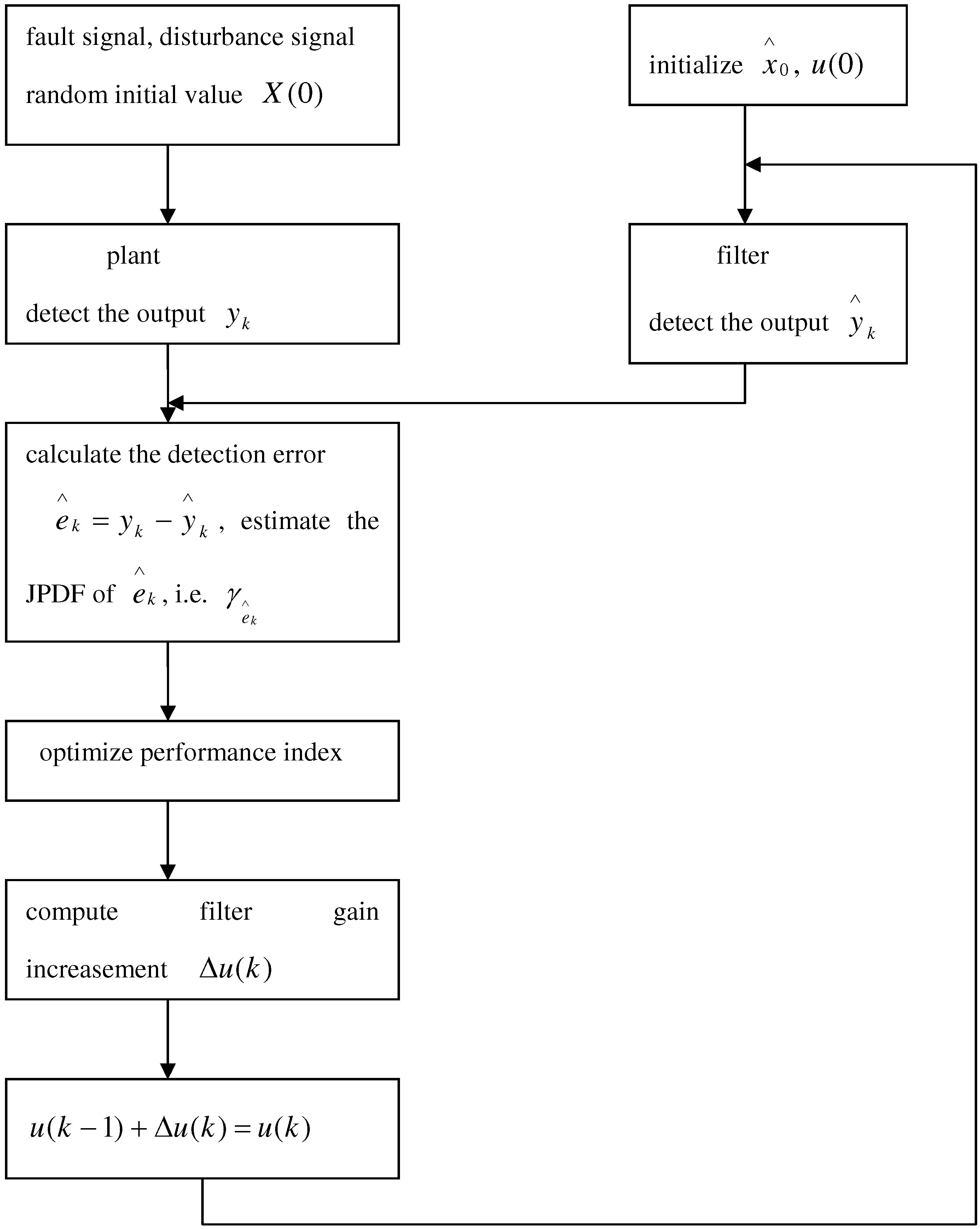
Remark 6. The real-time suboptimal FD filter design algorithm can be summarized as follows:

• Initialize $x_0,{\widehat{x}}_0=\epsilon \left(x_0\right)$ and $u_0;$
• At the sample time $k,$ compute ${\gamma }_{e_{k+1}}^i\left(\tau \right)$, $\tau \in {[\alpha ,\beta ]}^n$ based on Theorem 3;
• At the sample time $k,$ compute ${\gamma }_{{\widehat{e}}_{k+1}}^i\left(\tau \right)$, $\tau \in {[\alpha ,\beta ]}^m$ and then obtain $H^i\left({\widehat{e}}_{k+1}\right)$ $(i=0,1)$ via (18);
• Calculate $\Delta u_k$ and $u_k$ using equation (40) and (38);
• Increase k by 1 to the next step.

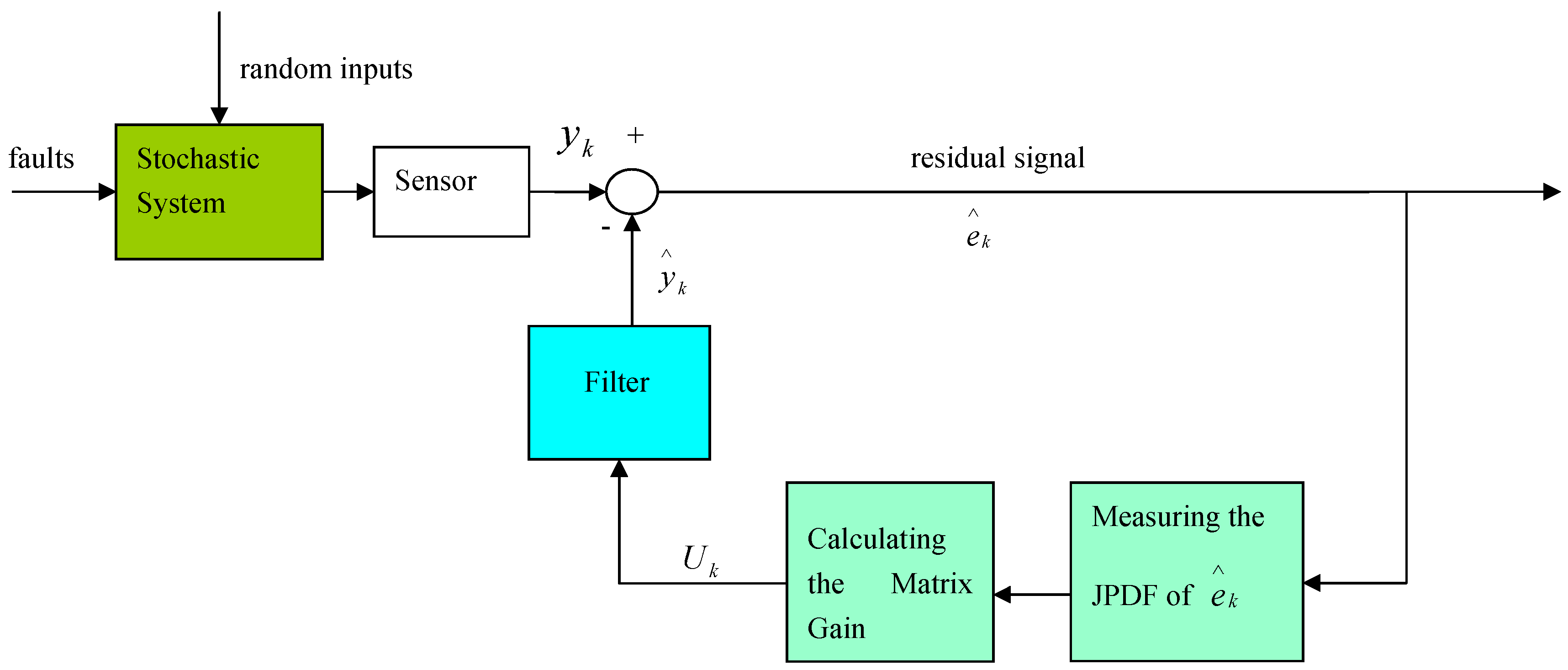
The schematic diagram and flow chart are given in Figure 1 and Figure 2 to illustrate how to apply our function based fault detection method to multivariate uncertain non-Gaussian system step by step.

Figure 1. Function based fault detection.

Figure 1. Function based fault detection.

Figure 2. Flow chart of function based fault detection.

Figure 2. Flow chart of function based fault detection.

4. Simulation Results

To demonstrate the FD algorithm, we consider a nonlinear non-Gaussian model described as

$$\left\{\begin{array}{cc}\left[\begin{array}{c}{x}_{1,k+1}\\ x_{2,k+1}\end{array}\right]\hfill & =\left[\begin{array}{cc}1& 0\\ 0& a_0\left(k\right)\end{array}\right]\left[\begin{array}{c}{x}_{1,k}\\ x_{2,k}\end{array}\right]+\left[\begin{array}{c}sin{x}_{1,k}\\ {cos}^2{x}_{2,k}\end{array}\right]+\left[\begin{array}{c}1\\ b_0\left(k\right)\end{array}\right]{\delta }_{k+1}+\left[\begin{array}{c}1\\ 1\end{array}\right]{\omega }_{k+1}+▵F\hfill \\ y_k\hfill & =x_{1,k}+x_{2,k}+v_k\hfill \end{array}\right.$$

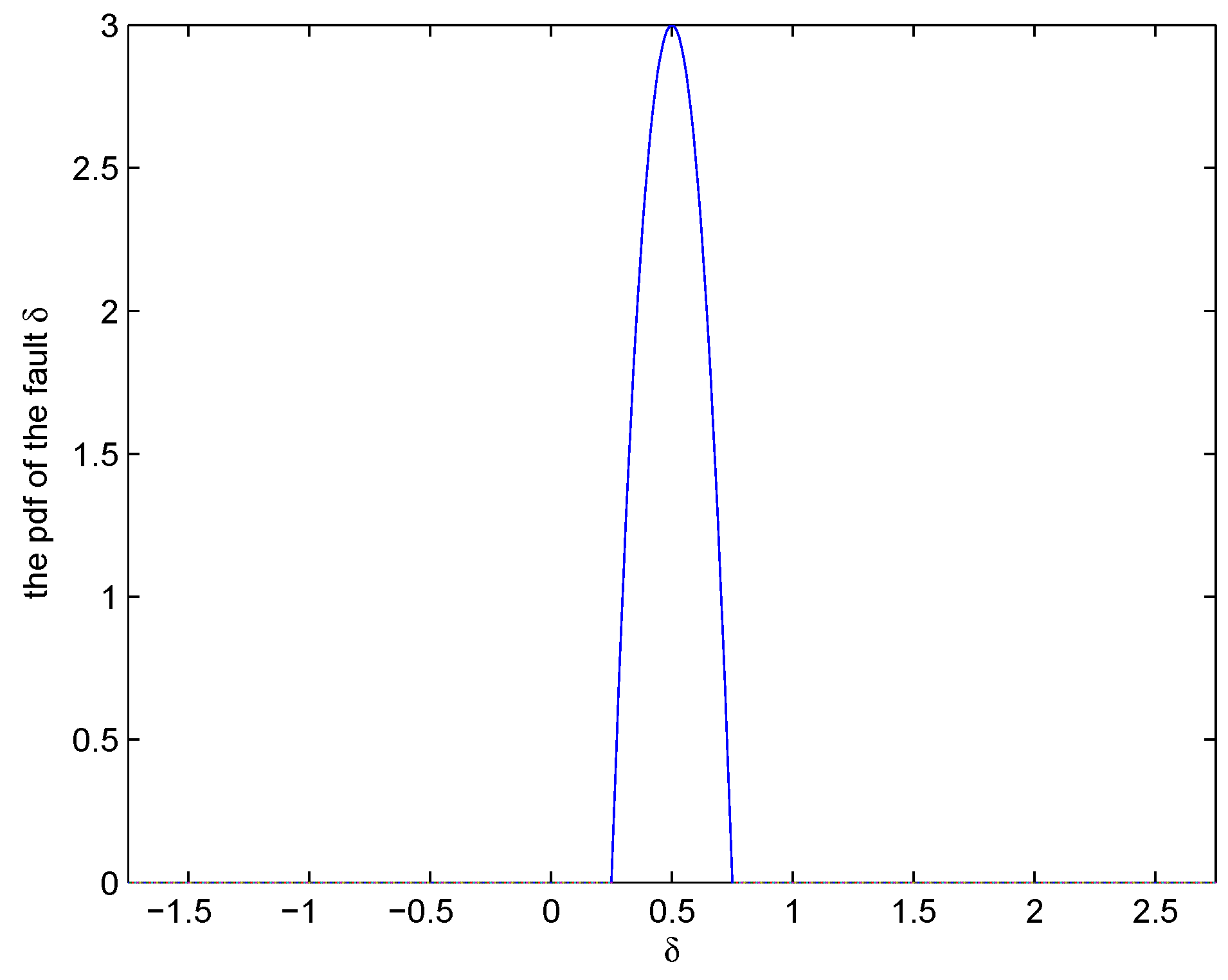
where $a_0\left(k\right)=-arctan{(1+k)}^{-1}+0.5,b_0\left(k\right)=0.02{(k+1)}^{-1/2},$ the fault ${\delta }_k$ and the disturbances ${\omega }_k,v_k(k=1,2,\cdots )$ are assumed to be mutually independent. The asymmetric PDF of ${\delta }_k$ is defined by ${\gamma }_{\delta }\left(x\right)=\left\{\begin{array}{cc}-48(x^2-x+\frac{3}{16})\hfill & x\in [0.25,0.75]\hfill \\ 0\hfill & x\in (-\infty ,0.25)\cup (0.75,+\infty )\hfill \end{array}\right.$

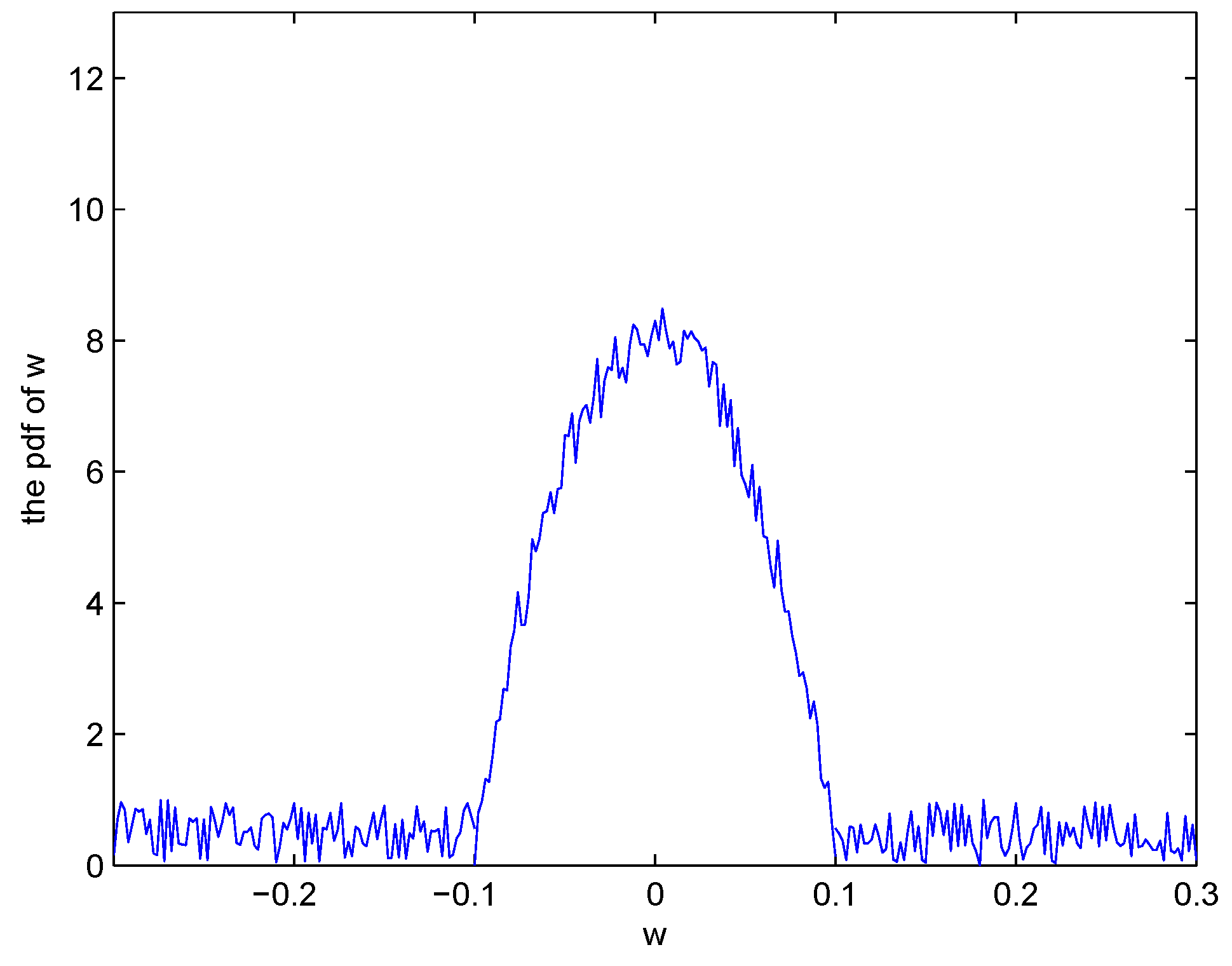
The PDF of the disturbance $w_k$ is supposed to have a perturbation, i.e., ${\gamma }_{\omega }\left(x\right)={\gamma }_{{\omega }_0}\left(x\right)+▵{\gamma }_{\omega }$ where ${\gamma }_{{\omega }_0}\left(x\right)=\left\{\begin{array}{cc}-\frac{3000(x^2-0.01)}{4}\hfill & x\in [-0.1,0.1]\hfill \\ 0\hfill & x\in (-\infty ,-0.1)\cup (0.1,+\infty )\hfill \end{array}\right.$ and $|▵{\gamma }_{\omega }|\le 0.01.$

The disturbance $v_k$ is a Gaussian variable with the distribution $N(0,0.01).$

According to (2), the filter can be formed as follows:

$$\left\{\begin{array}{cc}\left[\begin{array}{c}{\widehat{x}}_{1,k+1}\\ {\widehat{x}}_{2,k+1}\end{array}\right]\hfill & =\left[\begin{array}{cc}1& 0\\ 0& a_0\left(k\right)\end{array}\right]\left[\begin{array}{c}{\widehat{x}}_{1,k}\\ {\widehat{x}}_{2,k}\end{array}\right]+\left[\begin{array}{c}sin{\widehat{x}}_{1,k}\\ {cos}^2{\widehat{x}}_{2,k}\end{array}\right]+\left[\begin{array}{c}{u}_k\\ 0\end{array}\right](y_k-{\widehat{y}}_k)\hfill \\ {\widehat{y}}_k\hfill & ={\widehat{x}}_{1,k}+{\widehat{x}}_{2,k}\hfill \end{array}\right.$$

Thus, the estimation error system is driven by

$$\begin{array}{ccc}\hfill e_{k+1}& =& \left[\begin{array}{c}{x}_{1,k}+sin{x}_{1,k}\\ a_0\left(k\right)x_{2,k}+{cos}^2{x}_{2,k}\end{array}\right]+\left[\begin{array}{c}1\\ b_0\left(k\right)\end{array}\right]{\delta }_{k+1}+\left[\begin{array}{c}1\\ 1\end{array}\right]{\omega }_{k+1}-\left[\begin{array}{c}{\widehat{x}}_{1,k}+sin{\widehat{x}}_{1,k}\\ a_0\left(k\right){\widehat{x}}_{2,k}+{cos}^2{\widehat{x}}_{2,k}\end{array}\right]\hfill \\ & & -\left[\begin{array}{c}{u}_k\\ 0\end{array}\right](y_k-{\widehat{y}}_k)+▵F.\hfill \end{array}$$

and thus

$$\begin{array}{ccc}\hfill {\widehat{e}}_{k+1}& =& y_{k+1}-{\widehat{y}}_{k+1}\hfill \\ & =& x_{1,k+1}+x_{2,k+1}+v_{k+1}-{\widehat{x}}_{1,k+1}-{\widehat{x}}_{2,k+1}\hfill \\ & =& e_{1,k+1}+e_{2,k+1}+v_{k+1}\hfill \end{array}$$

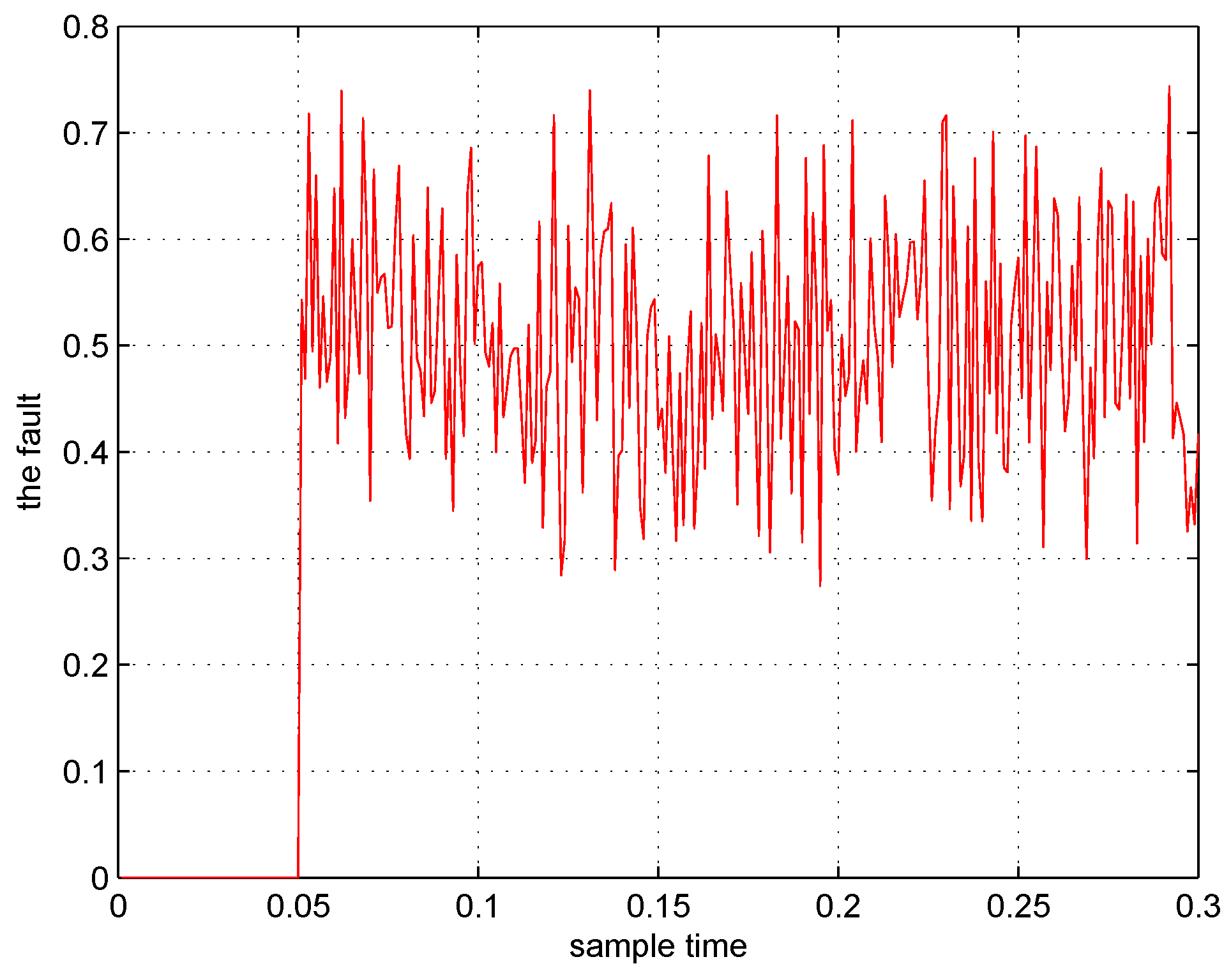
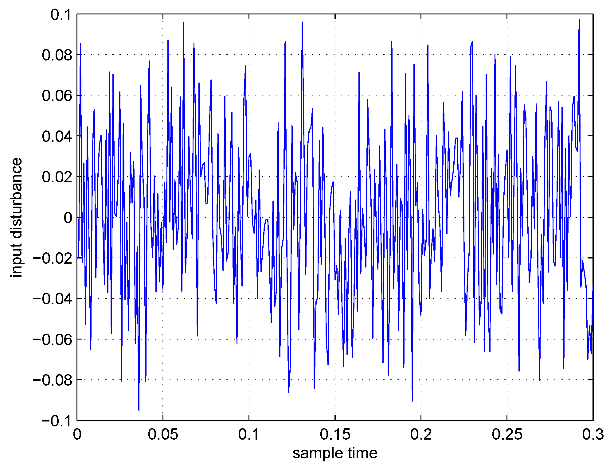
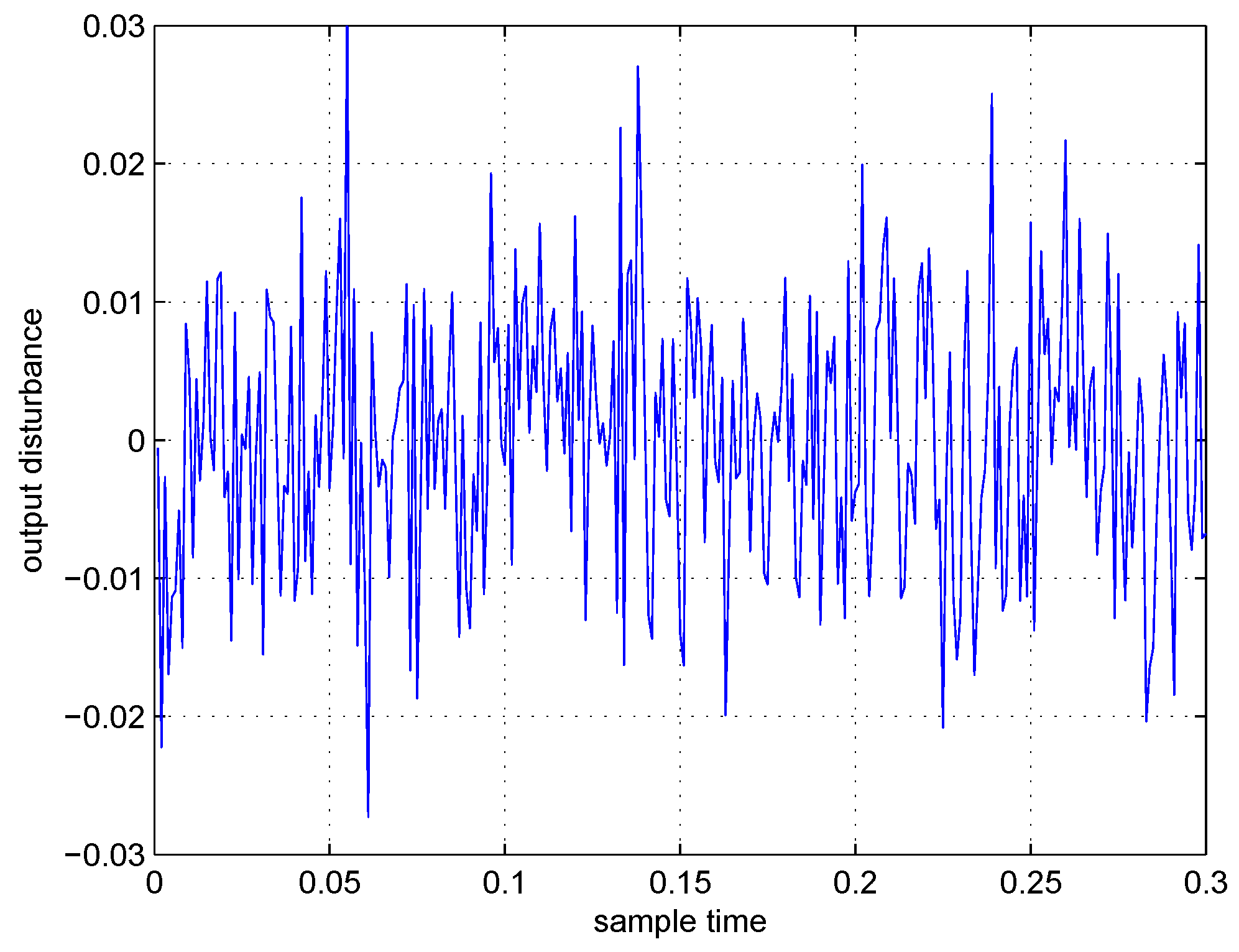
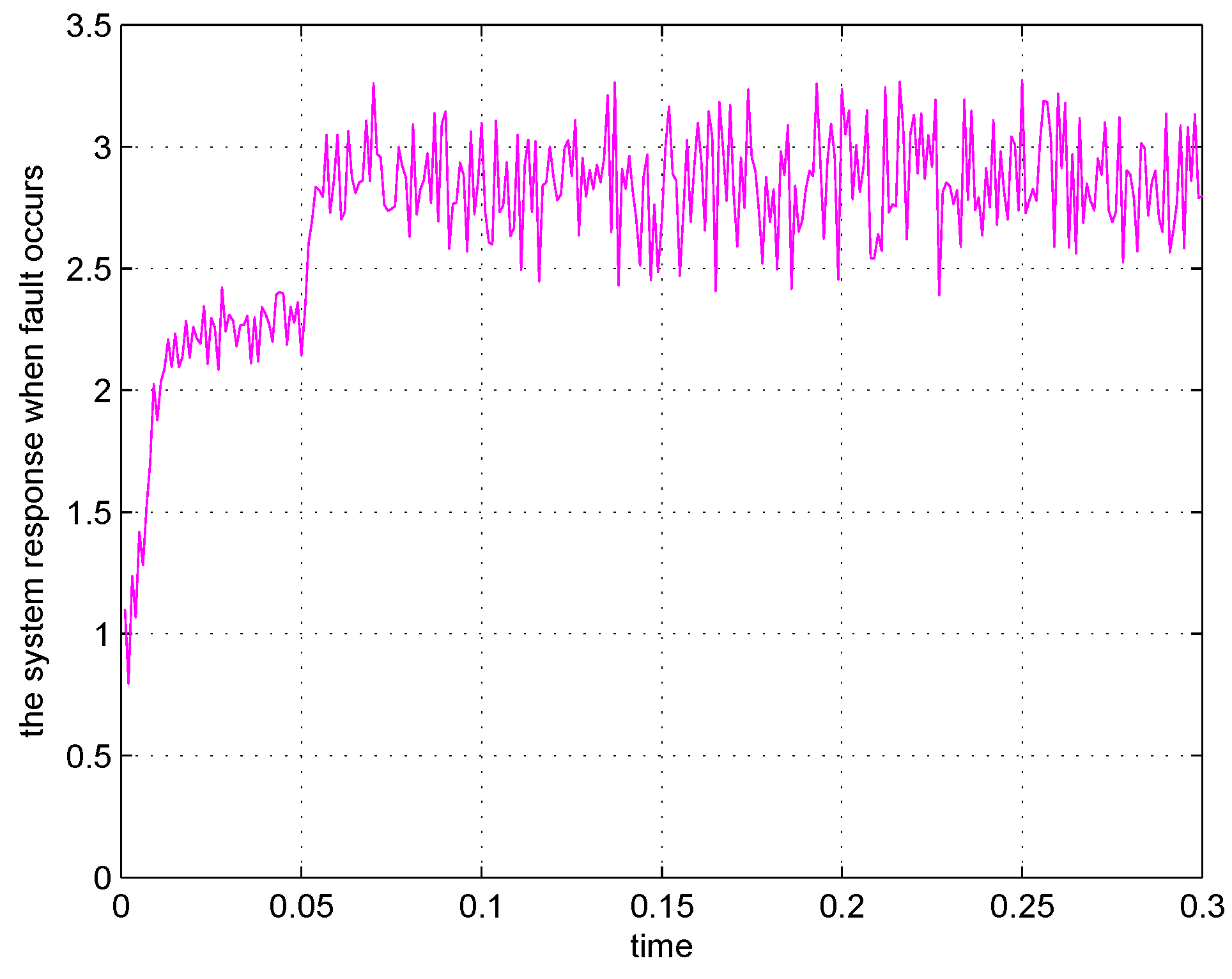
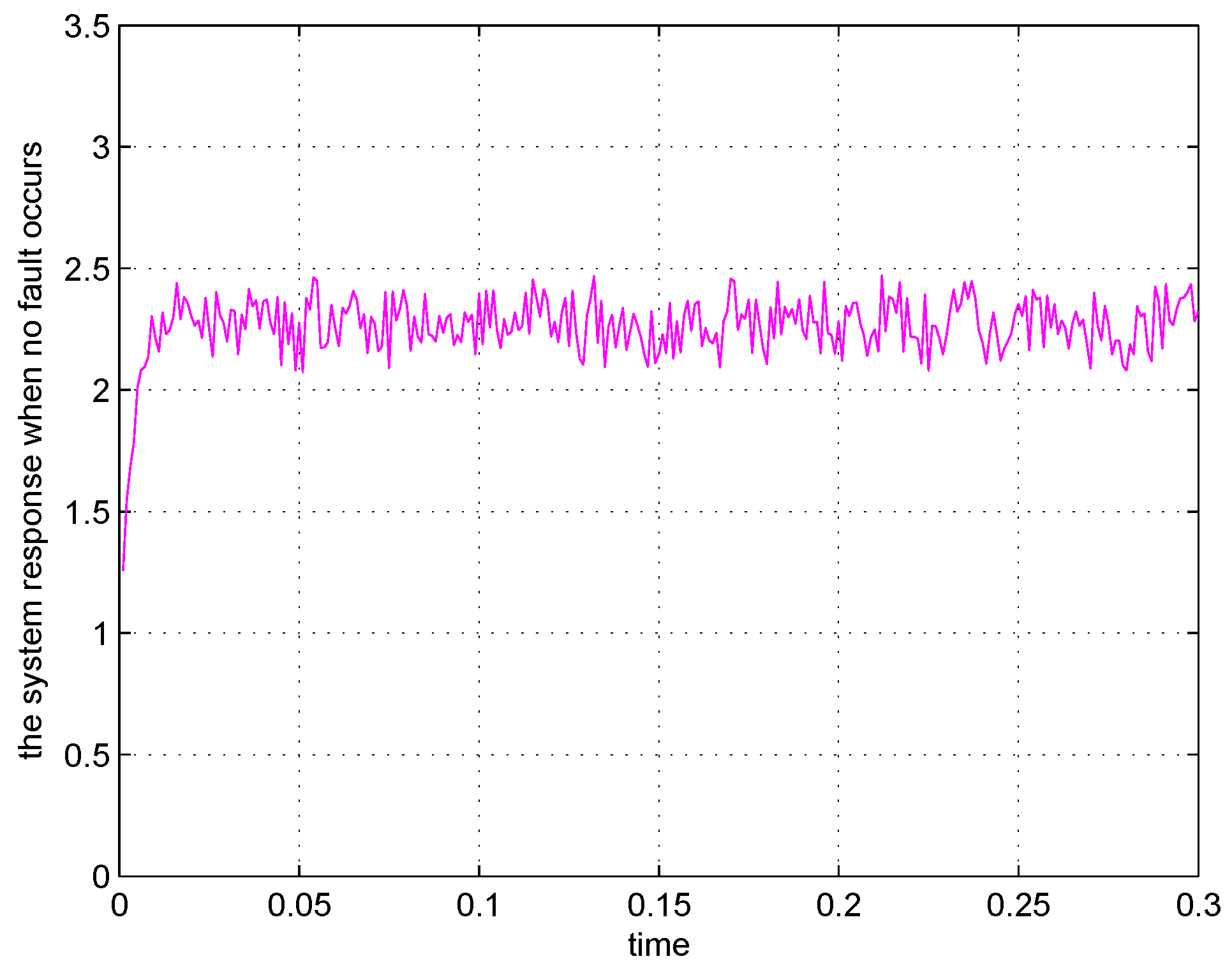
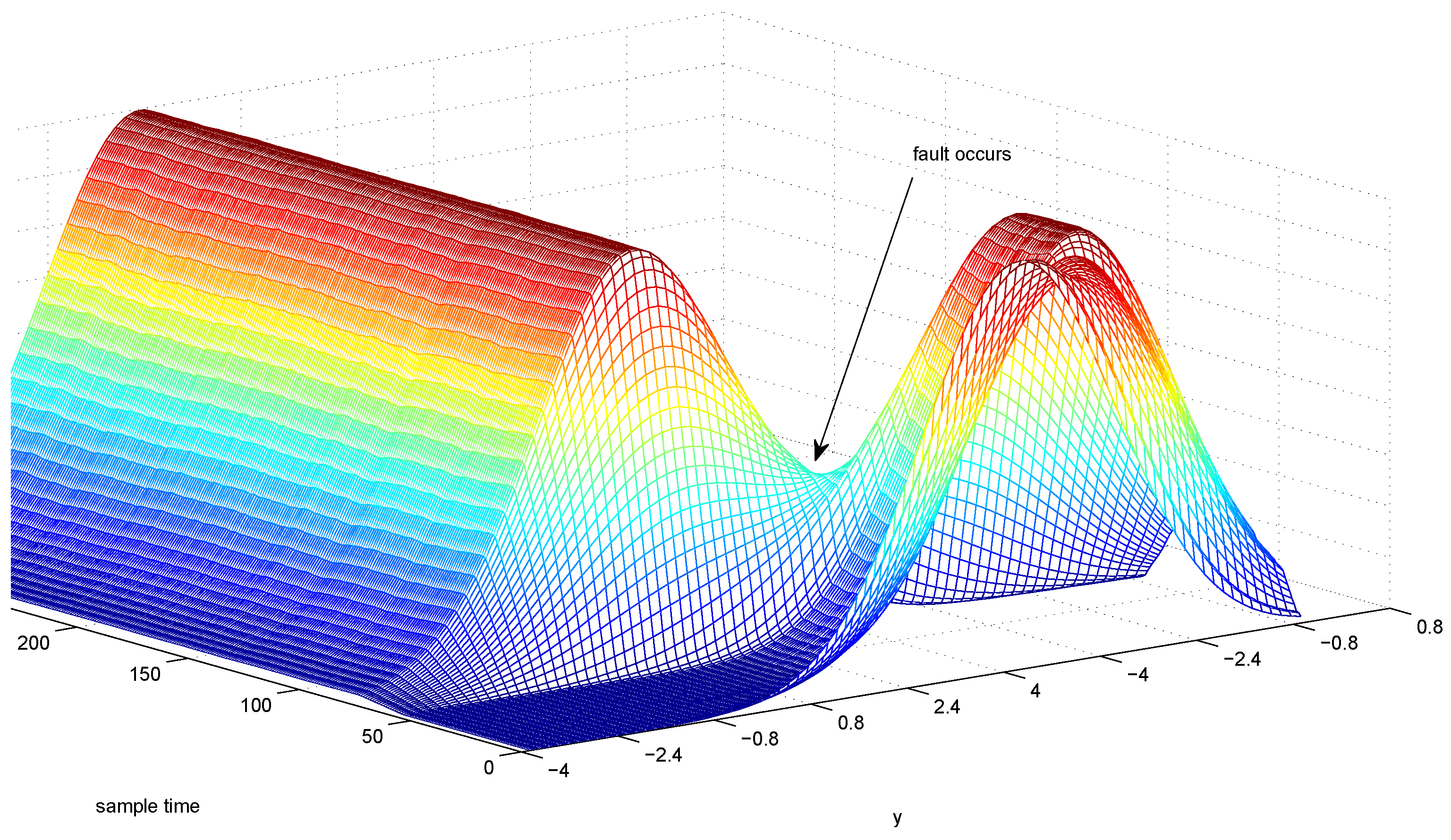
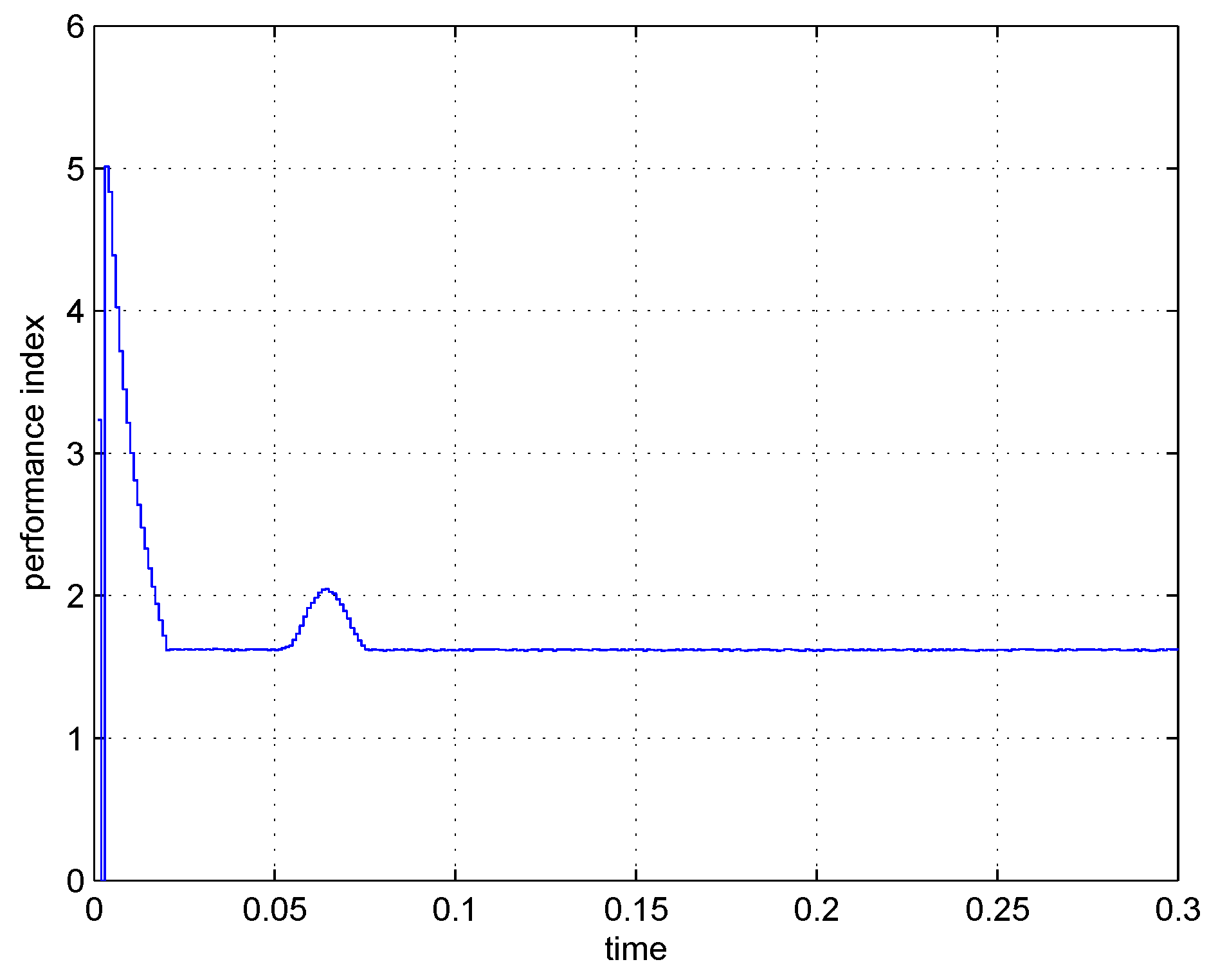
In the simulations, $x_0$ is set to be under uniform distribution on the interval ${[0,1]}^2$ and thus ${\widehat{x}}_0=\epsilon \left(x_0\right)={[0.5,0.5]}^T,u_0$ is set to be ${[0,0]}^T,$ the weights are set to be $R_1=1$ and $R_2=0.1.$ Figure 3, Figure 4 and Figure 5 show the signals for the fault and disturbances, while Figure 6, Figure 7 and Figure 8 show the corresponding pdfs of the signal. Figure 9 and Figure 10 are provided to demonstrate the residual signals ${\widehat{e}}_k$ in the absence and in the presence of fault emerging respectively. When the random fault occurs, it is shown that the detection error increases significantly. Figure 11 is the 3-D mesh of the system output y, which shows a remarkable change of the pdf ${\gamma }_y$ when the fault occurs at sample time 50. Figure 12 is the optimization performance index along time t. The result shows that a satisfactory FD performance can be obtained through the error dynamics by optimizing the entropies of the detection errors.

Figure 3. The response of the fault δ.

Figure 3. The response of the fault δ.

Figure 4. The response of the input disturbance ${\omega }_k$.

Figure 4. The response of the input disturbance ${\omega }_k$.

Figure 5. The response of the output disturbance $v_k$.

Figure 5. The response of the output disturbance $v_k$.

Figure 6. The PDF of the fault signal δ.

Figure 6. The PDF of the fault signal δ.

Figure 7. The PDF of the input disturbance ${\omega }_k$.

Figure 7. The PDF of the input disturbance ${\omega }_k$.

Figure 8. The PDF of the output disturbance $v_k$.

Figure 8. The PDF of the output disturbance $v_k$.

Figure 9. The residual value when fault occurs.

Figure 9. The residual value when fault occurs.

Figure 10. The residual value when no fault occurs.

Figure 10. The residual value when no fault occurs.

Figure 11. 3-D mesh of the system output y.

Figure 11. 3-D mesh of the system output y.

Figure 12. The optimization performance index J.

Figure 12. The optimization performance index J.

5. Conclusions

Since the classical FD approach using the Kalman-filter theory is insufficient to apply to the stochastic systems with non-Gaussian variables, a new FD framework is proposed in this paper for dynamic multivariate nonlinear stochastic systems. The entropy optimization principle is established for the concerned nonlinear detection error system, as represented by a non-Gaussian stochastic system. The main design principle is to maximize the entropies of the residual errors when the faults occur and to minimize the entropies of the residual errors resulting from other stochastic noises. For this purpose, new relationships are provided to calculate the JPDFs of the detection error in terms of the JPDFs of both the disturbances and the faults. As such, recursive approaches can be constructed to formulate the entropies of the detection errors. Combining the formulations with the novel performance indexes based on the entropy optimization principles, the recursive algorithms are provided to calculate the gain of the optimal FD filters. The advantages derived from the proposed fault detection approach are summarized as following

• The detected fault and system noises do not have to be Gaussian.
• The entropy optimization principle for FD problems is in parallel to the main results to [2], where linear Gaussian systems were studied and the minimax technology was applied to the variance of errors. It has therefore generalized variance optimization for Gaussian signal.
• The fault detection algorithm only uses the JPDF of the residual signal to calculate the filter gain matrix. There is no need to measure the system output pdf. This constitutes a major advantage compared with [37,38,39], which require the output pdf to be measurable.
• This fault detection approach is applicable to multivariate and uncertain systems. It is a generalization of the method in [8] where only single-input-signal-output system is concerned.

However, several issues still need to be studied in the future, i.e., how to determine the threshold and how to perform fault diagnosis. Moreover, as a branch of stochastic distribution control (SDC), fault detection using entropy optimization principle still remains in the theoretic research stage [8,37,40]. Its real world application requires more research efforts.

References

1. Basseville, M. On-board component fault detection and isolation using the statistic local approach. Automatic 1998, 34, 1391–1415. [Google Scholar] [CrossRef]
2. Chen, R.H.; Mingori, D.L.; Speyer, J.L. Optimal stochastic fault detection filter. Automatica 2003, 39, 377–390. [Google Scholar] [CrossRef]
3. Chen, R.H.; Speyer, J.L. A generalized least-squares fault detection filter. Int. J. Adapt. Contr. Signal Process. 2000, 14, 747–757. [Google Scholar] [CrossRef]
4. De Persis, C.; Isidori, A. A geometric approach to nonlinear fault detection and isolation. IEEE Trans. Automat. Contr. 2001, 46, 853–856. [Google Scholar] [CrossRef]
5. Frank, P.M. Fault diagnosis in dynamic systems using analytical and knowledge-based redundancy a survey and some new results. Automatica 1990, 26, 459–474. [Google Scholar] [CrossRef]
6. Guo, L.; Wang, H. Minimum entropy filtering for multivariate stochastic systems with non-Gaussian noises. IEEE Trans. Automat. Contr. 2006, 51, 695–700. [Google Scholar] [CrossRef]
7. Shields, D.N.; Ashton, S.A.; Daley, S. Robust fault detection observers for nonlinear polynomial systems. Int. J. Syst. Sci. 2001, 32, 723–737. [Google Scholar] [CrossRef]
8. Guo, L.; Wang, H.; Chai, T. Fault detection for non-linear non-Gaussian stochastic systems using entropy optimization principle. Trans. Inst. Meas. Contr. 2006, 28, 145–161. [Google Scholar] [CrossRef]
9. Mao, Z.H.; Jiang, B.; Shi, P. H-infinity fault detection filter design for networked control systems modelled by discrete Markovian jump systems. IET Proc. Contr. Theor. Appl. 2007, 1, 1336–1343. [Google Scholar] [CrossRef]
10. Jiang, B.; Staroswiecki, M.; Cocquempot, V. Fault accommodation for a class of nonlinear systems. IEEE Trans. Automat. Contr. 2006, 51, 1578–1583. [Google Scholar] [CrossRef]
11. Basseville, M.; Nikiforv, I. Fault isolation and diagnosis: Nuisance rejection and multiple hypothesis testing. Annu. Rev. Contr. 2002, 26, 189–202. [Google Scholar] [CrossRef]
12. Bar-Shalom, Y.; Li, X.R. Estimation and Tracking: Princples, Techniques, and Software; Artech House: Norwood, MA, USA, 1996. [Google Scholar]
13. Zhang, J.; Cai, L.; Wang, H. Minimum entropy filtering for networked control systems via information theoretic learning approach. In Proceedings of the 2010 International Conference on Modelling, Identification and Control, Okayama, Japan, 17–19 July 2010; pp. 774–778.
14. Orchardand, M.; Vachtsevanos, G. A particle filtering approach for on-line fault diagnosis and failure prognosis. Trans. Inst. Meas. Contr. 2009, 31, 221–246. [Google Scholar] [CrossRef]
15. Chen, C.; Zhang, B.; Vachtsevanos, G.; Orchard, M. Machine condition prediction based on adaptive neuro-fuzzy and high-order particle filtering. IEEE Trans. Ind. Electron. 2011, 58, 4353–4364. [Google Scholar] [CrossRef]
16. Wang, H.; Afshar, P. ILC-based fixed-structure controller design for output PDF shaping in stochastic systems using LMI techniques. IEEE Trans. Automat. Contr. 2009, 54, 760–773. [Google Scholar] [CrossRef]
17. Zhou, J.; Zhou, D.; Wang, H.; Guo, L.; Chai, T. Distribution function tracking filter design using hybrid characteristic functions. Automatica 2010, 46, 101–109. [Google Scholar] [CrossRef]
18. Chen, C.; Brown, D.; Sconyers, C.; Zhang, B.; Vachtsevanos, G.; Orchard, M. An integrated architecture for fault diagnosis and failure prognosis of complex engineering systems. Expert Syst. Appl. 2012, 39, 9031–9040. [Google Scholar] [CrossRef]
19. Yin, L.; Guo, L. Fault isolation for dynamic multivariate nonlinear non-gaussian stochastic systems using generalized entropy optimization principle. Automatica 2009, 45, 2612–2619. [Google Scholar] [CrossRef]
20. Yin, L.; Guo, L. Fault detection for NARMAX stochastic systems using entropy optimization principle. In Proceedings of the 2009 Chinese Control and Decision Conference, Guilin, China, June 2009; pp. 870–875.
21. Guo, L.; Chen, W. Disturbance attenuation and rejection for systems with nonlinearity via DOBC approach. Int. J. Robust Nonlinear Contr. 2005, 15, 109–125. [Google Scholar] [CrossRef]
22. Yang, F.; Wang, Z.; Hung, S. Robust kalman filtering for discrete time-varying uncertain systems with multiplicative noise. IEEE Trans. Automat. Contr. 2002, 47, 1179–1183. [Google Scholar] [CrossRef]
23. Guo, L.; Wang, H.; Wang, A.P. Optimal probability density fuction control for NARMAX stochastic systems. Automatica 2008, 44, 1904–1911. [Google Scholar] [CrossRef]
24. Yin, L.; Guo, L. Joint stochastic distribution tracking control for multivariate descriptor systems with non-gaussian variables. Int. J. Syst. Sci. 2012, 43, 192–200. [Google Scholar] [CrossRef]
25. Guo, L.; Yin, L.; Wang, H. Robust PDF control with guaranteed stability for nonlinear stochastic systems under modeling errors. IET Contr. Theor. Appl. 2009, 3, 575–582. [Google Scholar] [CrossRef]
26. Yin, L.; Guo, L.; Wang, H. Robust minimum entropy tracking control with guaranteed stability for nonlinear stochastic systems under modeling errors. In Proceedings of the 10th International Conference on Control, Automation, Robotics and Vision, Hanoi, Vietnam, 17–20 December 2008; pp. 1469–1474.
27. Papoulis, A. Probablity, Random Variables and Stochastic Processes, 3rd ed.; McGraw-Hill: New York, NY, USA, 1991. [Google Scholar]
28. Patton, R.J.; Frank, P.; Clark, R. Fault Diagnosis in Dynamic Systems: Theory and Application; Prentice Hall: Englewood Cliff, NJ, USA, 1989. [Google Scholar]
29. Feng, X.B.; Loparo, K.A. Active probing for information in control system with quantized state measurements: A minimum entropy approach. IEEE Trans. Automat. Contr. 1997, 42, 216–238. [Google Scholar] [CrossRef]
30. Wang, H. Minimum entropy control of non-Gaussian dynamic stochastic systems. IEEE Trans. Automat. Contr. 2002, 47, 398–403. [Google Scholar] [CrossRef]
31. Saridis, G.N. Entropy formulation of optimal and adaptive control. IEEE Trans. Automat. Contr. 1988, 33, 713–720. [Google Scholar] [CrossRef]
32. Wang, H. Bounded Dynamic Stochastc Systems: Modelling and Control; Springer-Verlag: London, UK, 2000. [Google Scholar]
33. Zhang, J.; Du, L.; Ren, M.; Hou, G. Minimum error entropy filter for fault detection of networked control systems. Entropy 2012, 14, 505–516. [Google Scholar] [CrossRef]
34. Silverman, B.W. Density Estimation for Statistics and Data Analysis; Chapman and Hall: London, UK, 1986. [Google Scholar]
35. Wang, H.; Lin, W. Applying observer based FDI techniques to detect faults in dynamic and bounded stochastc distributions. Int. J. Contr. 2000, 73, 1424–1436. [Google Scholar] [CrossRef]
36. Yue, H.; Wang, H. Minimum entropy control of closed-loop tracking errors for dynamic stochastic systems. IEEE Trans. Automat. Contr. 2003, 48, 118–121. [Google Scholar]
37. Guo, L.; Zhang, Y.M.; Wang, H.; Fang, J.C. Observer-based optimal fault detection and diagnosis using conditional probability distributions. IEEE Trans. Signal Process. 2006, 54, 3712–3719. [Google Scholar] [CrossRef]
38. Zhang, Y.M.; Guo, L.; Wang, H. Filter-based fault detection and diagnosis using output PDFs for stochastic systems with time delays. Int. J. Adapt. Contr. Signal Process. 2006, 20, 175–194. [Google Scholar] [CrossRef]
39. Li, T.; Guo, L.; Wu, L.Y. Observer-based optimal fault detection using PDFs for time-delay stochastic systems. Nonlinear Anal. R. World Appl. 2008, 9, 2337–2349. [Google Scholar] [CrossRef]
40. Guo, L.; Yin, L.; Wang, H.; Chai, T.Y. Entropy optimization filtering for fault isolation of nonlinear non-gaussian stochastic systems. IEEE Trans. Automat. Contr. 2009, 54, 804–810. [Google Scholar]