Ordered Regions within a Nonlinear Time Series Solution of a Lorenz Form of the Townsend Equations for a Boundary-Layer Flow

Abstract
:1. Introduction
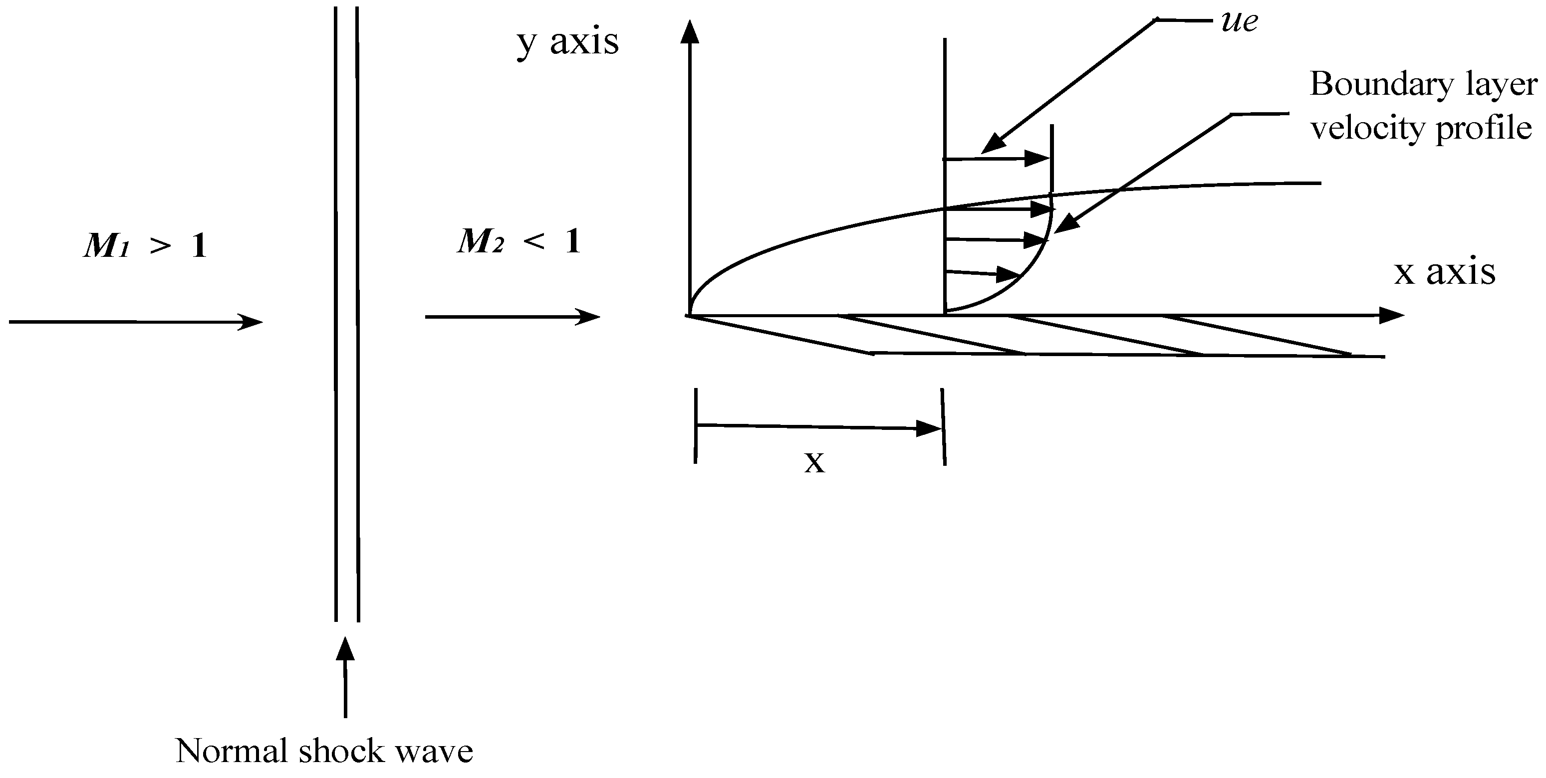
2. Supersonic Flow Environment
3. Thermo-Physical Properties
4. Computational Model for the Boundary-Layer Flow

5. Mathematical Model of the Flow Instability
5.1. Transformation of the Townsend Equations


5.2. Extracting Ordered Signals from Nonlinear Instability Time Series


5.3. The Prediction of Spectral Entropy Rates from the Deterministic Results


6. Discussion
7. Conclusions
Nomenclature:
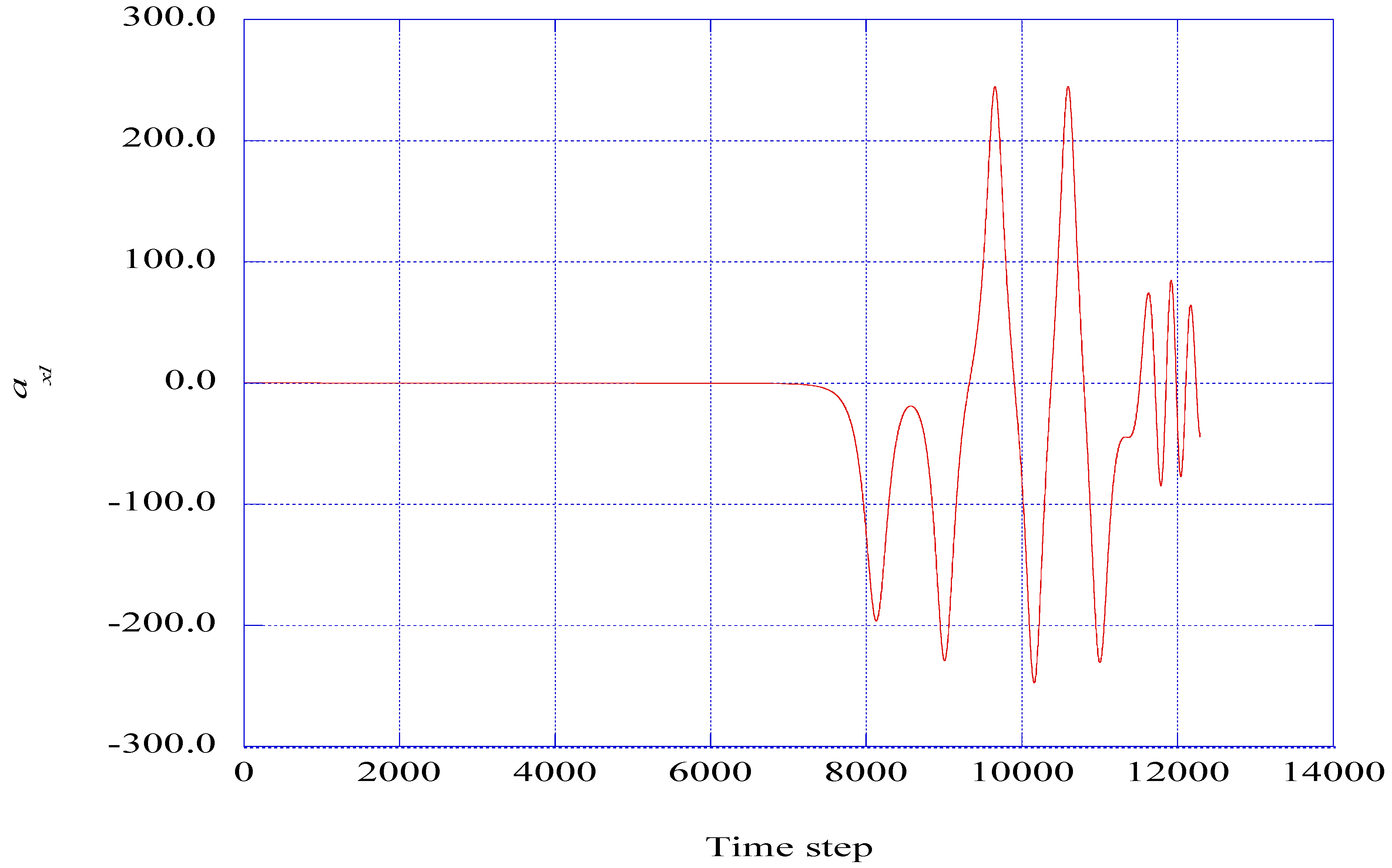
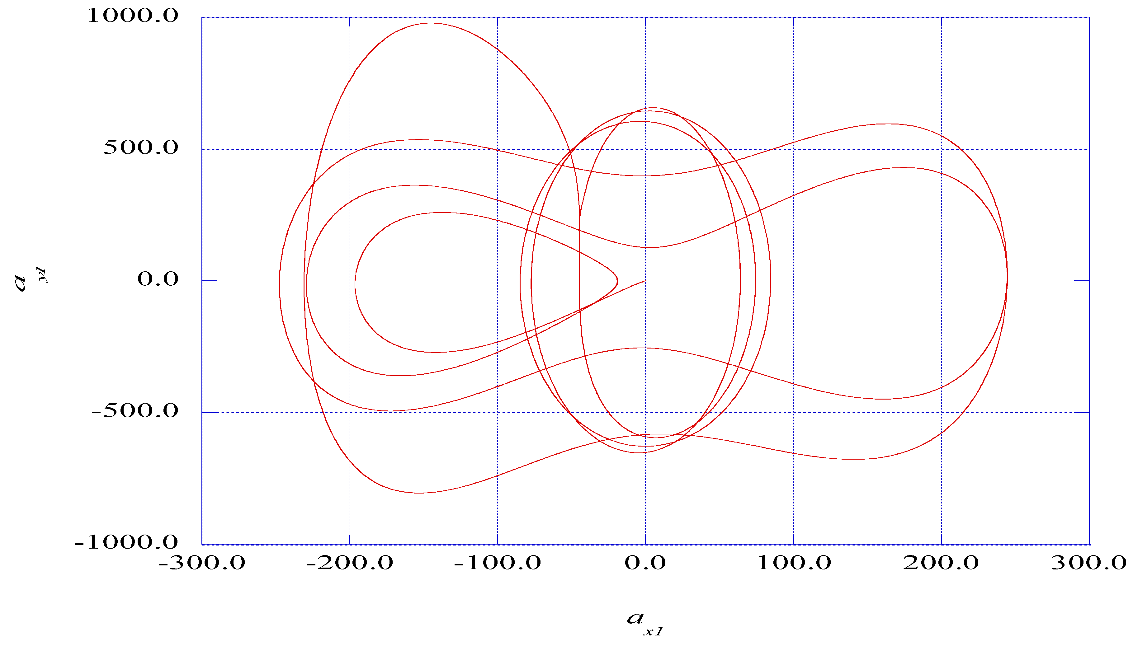
| ai | Fluctuating i-th component of velocity wave vector |
| b1 | Coefficient in modified Townsend equations defined by Equation (32) |
| fr | Power spectral density of the fluctuating axial velocity wave vector |
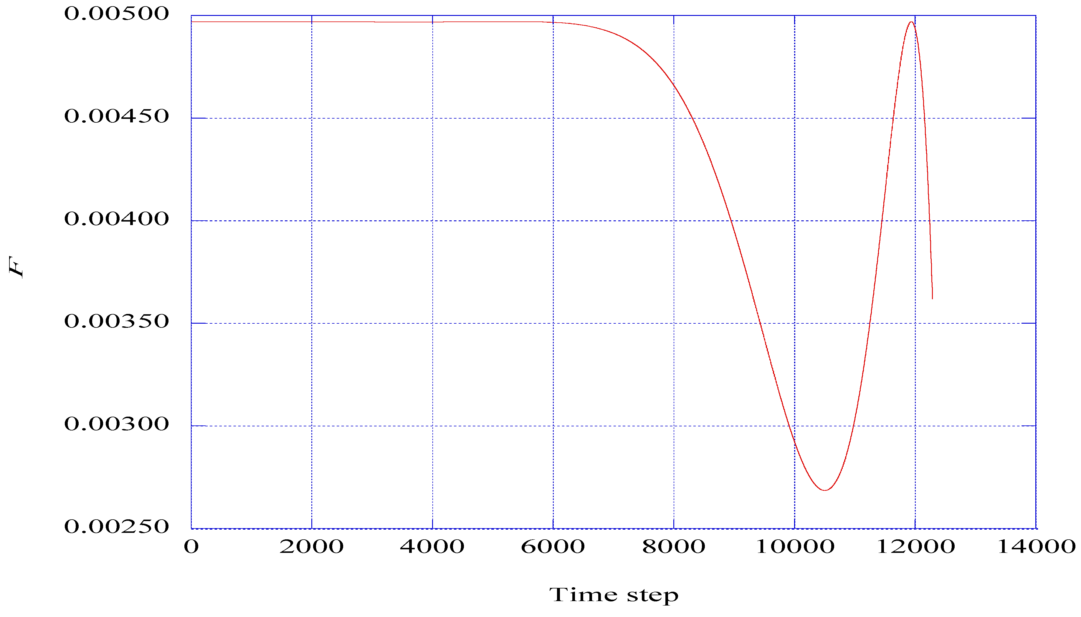
| F | Time-dependent perturbation factor |
| j | Vertical station number in the boundary-layer computations |
| j | Time series data segment |
| k | Time-dependent wave number magnitude |
| ki | Fluctuating i-th wave number of Fourier expansion |
| K | Adjustable weighting factor |
| M1 | Flight Mach number |
| M2 | Mach number downstream of a normal shock wave |
| nx | Axial station number in the boundary-layer computations |
| p | Hydrostatic pressure |
| p1 | Static pressure ahead of the normal shock wave |
| p2 | Static pressure behind the normal shock wave |
| Pr | Probability of the power spectral density of the r-th spectral segment |
| r1 | Coefficient in modified Townsend equations defined by Equation (30) |
| s1 | Coefficient in modified Townsend equations defined by Equation (31) |
| sj_ | spent Spectral entropy rate over the j-th spectral segment |
| t | Time |
| t1 | Static temperature ahead of the normal shock wave |
| t2 | Static temperature behind the normal shock wave |
| Taw | Adiabatic wall temperature |
| u | Axial boundary-layer velocity |
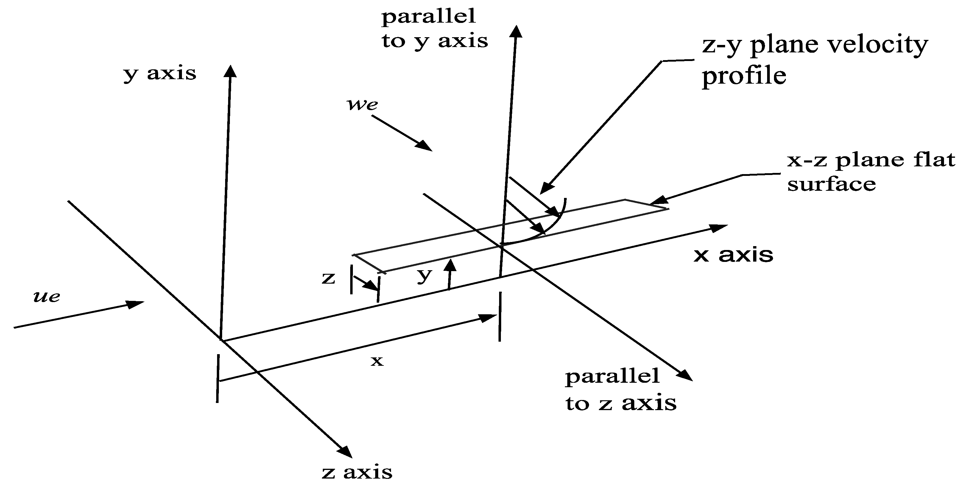
| ue | Axial velocity at the outer edge of the x-y plane boundary layer |
| ui | Fluctuating i-component of velocity instability |
| Ui | Mean velocity in the i-direction |
| v | Vertical boundary-layer velocity |
| Vy | Mean vertical velocity in the x-y plane |
| Vz | Mean vertical velocity in the z-y plane |
| w | Span wise boundary-layer velocity |
| we | Span wise velocity at the outer edge of the z-y plane boundary layer |
| W | Mean velocity in the span wise direction |
| x | Axial distance |
| xi | i-th direction |
| xj | j-th direction |
| y | Vertical distance |
| yxz | Vertical distance to the x-z surface |
| z | Span wise distance |
Greek Letters
| δlm | Kronecker delta |
| η | Transformed vertical parameter |
| ν | Kinematic viscosity of the gas mixture |
| σy1 | Coefficient in modified Townsend equations defined by Equation (28) |
| σx1 | Coefficient in modified Townsend equations defined by Equation (29) |
Subscripts
| i, j, l, m | Tensor indices |
| r | The r-th index in the j-th time series data segment |
| x | Component in the x-direction |
| y | Component in the y-direction |
| z | Component in the z-direction |
References
- Berlin, S.; Henningson, D.S. A nonlinear mechanism for receptivity of free-stream disturbances. Phys. Fluids 1999, 11, 3749–3760. [Google Scholar] [CrossRef]
- Hoepffner, J.; Brandt, L. Stochastic approach to the receptivity problem applied to bypass transition in boundary layers. Phys. Fluids 2008, 20, 024108:1–024108:4. [Google Scholar] [CrossRef]
- Waleffe, F. Homotopy of exact coherent structures in plane shear flows. Phys. Fluids 2003, 15, 1517–1534. [Google Scholar] [CrossRef]
- Cherubini, S.; De Palma, P.; Robinet, J.-C.; Bottaro, A. Edge states in a boundary layer. Phys. Fluids 2011, 23, 051750:1–051750:4. [Google Scholar] [CrossRef] [Green Version]
- Duguet, Y.; Schlatter, P.; Henningson, D.S. Localized edge states in plane Couette flow. Phys. Fluids 2009, 21, 111701:1–111701:5. [Google Scholar] [CrossRef]
- Cebeci, T.; Bradshaw, P. Momentum Transfer in Boundary Layers; Hemisphere: Washington, DC, USA, 1977. [Google Scholar]
- Hansen, A.G. Similarity Analyses of Boundary Value Problems in Engineering; Prentice-Hall, Inc.: Englewood Cliffs, NJ, USA, 1964; pp. 86–92. [Google Scholar]
- Townsend, A.A. The Structure of Turbulent Shear Flow, 2nd ed.; Cambridge University Press: Cambridge, UK, 1976; pp. 45–49. [Google Scholar]
- Isaacson, L.K. Spectral Entropy in a Boundary-Layer Flow. Entropy 2011, 13, 402–421. [Google Scholar] [CrossRef]
- Isaacson, L.K. Control Parameters for Boundary-Layer Instabilities in Unsteady Shock Interactions. Entropy 2012, 14, 131–160. [Google Scholar] [CrossRef]
- Chen, C.H. Digital Waveform Processing and Recognition; CRC Press, Inc.: Boca Raton, FL, USA, 1982; pp. 131–158. [Google Scholar]
- Press, W.; Teukolsky, S.A.; Vetterling, W.T.; Flannery, B.P. Numerical Recipes in C: The Art of Scientific Computing, 2nd ed.; Cambridge University Press: Cambridge, UK, 1992; pp. 572–575. [Google Scholar]
- Powell, G.E.; Percival, I.C. A spectral entropy method for distinguishing regular and irregular motions for Hamiltonian systems. J. Phys. Math. Gen. 1979, 12, 2053–2071. [Google Scholar] [CrossRef]
- Pecora, L.M.; Carroll, T.L. Synchronization in chaotic systems. In Controlling Chaos: Theoretical and Practical Methods in Non-linear Dynamics; Kapitaniak, T., Ed.; Academic Press Inc.: San Diego, CA, USA, 1996; pp. 142–145. [Google Scholar]
- Pérez, G.; Cerdeiral, H.A. Extracting messages masked by chaos. In Controlling Chaos: Theoretical and Practical Methods in Non-linear Dynamics; Kapitaniak, T., Ed.; Academic Press Inc.: San Diego, CA, USA, 1996; pp. 157–160. [Google Scholar]
- Cuomo, K.M.; Oppenheim, A.V. Circuit implementation of synchronized chaos with applications to communications. In Controlling Chaos: Theoretical and Practical Methods in Non-linear Dynamics; Kapitaniak, T., Ed.; Academic Press Inc.: San Diego, CA, USA, 1996; pp. 153–156. [Google Scholar]
- Feng, J.C.; Tse, C.K. Reconstruction of Chaotic Signals with Applications to Chaos-Based Communications; World Scientific Publishing Co. Pte. Ltd.: Hackensack, NJ, USA, 2008; pp. 165–213. [Google Scholar]
- Zucrow, M.J.; Hoffman, J.D. Gas Dynamics: Vol. I; John Wiley & Sons, Inc.: New York, NY, USA, 1976; pp. 335–349. [Google Scholar]
- Sonntag, R.E.; Van Wylen, G.J. Fundamentals of Statistical Thermodynamics; Robert Krieger Publishing Company, Inc.: Malabar, FL, USA, 1985. [Google Scholar]
- McBride, B.J.; Gordon, S.; Reno, M.A. Coefficients for Calculating Thermodynamic and Transport Properties of Individual Species; NASA TM 4513; National Aeronautics and Space Administration: Washington, DC, USA, October 1993. [Google Scholar]
- Dorrance, W.H. Viscous Hypersonic Flow; McGraw-Hill Book Company, Inc.: New York, NY, USA, 1962; pp. 276–315. [Google Scholar]
- Zucrow, M.J.; Hoffman, J.D. Gas Dynamics: Vol. I; John Wiley & Sons, Inc.: New York, NY, USA, 1976; pp. 708–709. [Google Scholar]
- Anderson, J.D., Jr. Hypersonic and High-Temperature Gas Dynamic, 2nd ed.; American Institute of Aeronautics and Astronautics, Inc.: Reston, VA, USA, 2006; p. 616. [Google Scholar]
- Sagaut, P.; Cambon, C. Homogeneous Turbulence Dynamics; Cambridge University Press: New York, NY, USA, 2008. [Google Scholar]
- Mathieu, J.; Scott, J. An Introduction to Turbulent Flow, Cambridge University Press: New York, NY 10011-4211, USA, 2000; 251–261.
- Landau, L.D.; Lifshitz, E.M. Quantum Mechanics: Non-Relativistic Theory; Addison-Wesley Publishing Company, Inc.: Reading MA, USA, 1958; pp. 143–144. [Google Scholar]
- Pyragas, K. Continuous control of chaos by self-controlling feedback. In Controlling Chaos: Theoretical and Practical Methods in Non-linear Dynamics; Kapitaniak, T., Ed.; Academic Press Inc.: San Diego, CA, USA, 1996; pp. 118–123. [Google Scholar]
- Hellberg, C.S.; Orszag, S.A. Chaotic behavior of interacting elliptical instability modes. Phys. Fluids 1988, 31, 6–8. [Google Scholar] [CrossRef]
- Isaacson, L. K. Deterministic Prediction of the Entropy Increase in a Sudden Expansion. Entropy 2011, 13, 402–421. [Google Scholar] [CrossRef]
- Press, W.; Teukolsky, S.A.; Vetterling, W.T.; Flannery, B.P. Numerical Recipes in C: The Art of Scientific Computing, 2nd ed.; Cambridge University Press: Cambridge, UK, 1992; pp. 710–714. [Google Scholar]
- Cover, T.M.; Thomas, J.A. Elements of Information Theory, 2nd ed.; John Wiley & Sons, Inc.: Hoboken, NJ, USA, 2006; pp. 415–421. [Google Scholar]
- Rissanen, J. Complexity and Information in Data. In Entropy; Greven, A., Keller, G., Warnecke, G., Eds.; Princeton University Press: Princeton, NJ, USA, 2003; pp. 299–327. [Google Scholar]
- Rissanen, J. Information and Complexity in Statistical Modeling; Springer Science+Business Media, LLC: New York, NY, USA, 2007. [Google Scholar]
- Li, M.; Vitányi, P. An Introduction to Kolmogorov Complexity and Its Applications; Springer Science+Business Media, LLC: New York, NY, USA, 2008. [Google Scholar]
- Press, W.; Teukolsky, S.A.; Vetterling, W.T.; Flannery, B.P. Numerical Recipes in C: The Art of Scientific Computing, 2nd ed.; Cambridge University Press: Cambridge, UK, 1992; pp. 572–575. [Google Scholar]
- Grassberger, P.; Procaccia, I. Estimation of the Kolmogorov entropy from a chaotic signal. Phys. Rev. A 1983, 28, 2591–2593. [Google Scholar] [CrossRef]
© 2013 by the authors; licensee MDPI, Basel, Switzerland. This article is an open access article distributed under the terms and conditions of the Creative Commons Attribution license (http://creativecommons.org/licenses/by/3.0/).
Share and Cite
Isaacson, L.K. Ordered Regions within a Nonlinear Time Series Solution of a Lorenz Form of the Townsend Equations for a Boundary-Layer Flow. Entropy 2013, 15, 53-79. https://doi.org/10.3390/e15010053
Isaacson LK. Ordered Regions within a Nonlinear Time Series Solution of a Lorenz Form of the Townsend Equations for a Boundary-Layer Flow. Entropy. 2013; 15(1):53-79. https://doi.org/10.3390/e15010053
Chicago/Turabian StyleIsaacson, LaVar King. 2013. "Ordered Regions within a Nonlinear Time Series Solution of a Lorenz Form of the Townsend Equations for a Boundary-Layer Flow" Entropy 15, no. 1: 53-79. https://doi.org/10.3390/e15010053