Estimation Bias in Maximum Entropy Models

Abstract

Maximum entropy models have become popular statistical models in neuroscience and other areas in biology and can be useful tools for obtaining estimates of mutual information in biological systems. However, maximum entropy models fit to small data sets can be subject to sampling bias; i.e., the true entropy of the data can be severely underestimated. Here, we study the sampling properties of estimates of the entropy obtained from maximum entropy models. We focus on pairwise binary models, which are used extensively to model neural population activity. We show that if the data is well described by a pairwise model, the bias is equal to the number of parameters divided by twice the number of observations. If, however, the higher order correlations in the data deviate from those predicted by the model, the bias can be larger. Using a phenomenological model of neural population recordings, we find that this additional bias is highest for small firing probabilities, strong correlations and large population sizes—for the parameters we tested, a factor of about four higher. We derive guidelines for how long a neurophysiological experiment needs to be in order to ensure that the bias is less than a specified criterion. Finally, we show how a modified plug-in estimate of the entropy can be used for bias correction.

1. Introduction

Understanding how neural populations encode information about external stimuli is one of the central problems in computational neuroscience [1,2]. Information theory [3,4] has played a major role in our effort to address this problem, but its usefulness is limited by the fact that the information-theoretic quantity of interest, mutual information (usually between stimuli and neuronal responses), is hard to compute from data [5]. That is because the key ingredient of mutual information is the entropy, and estimation of entropy from finite data suffers from a severe downward bias when the data is undersampled [6,7]. While a number of improved estimators have been developed (see [5,8] for an overview), the amount of data one needs is, ultimately, exponential in the number of neurons, so even modest populations (tens of neurons) are out of reach—this is the so-called curse of dimensionality. Consequently, although information theory has led to a relatively deep understanding of neural coding in single neurons [2], it has told us far less about populations [9,10]. In essence, the brute force approach to measuring mutual information that has worked so well on single spike trains simply does not work on populations.

One way around this problem is to use parametric models in which the number of parameters grows (relatively) slowly with the number of neurons [11,12]; and, indeed, parametric models have been used to bound entropy [13]. For such models, estimating entropy requires far less data than for brute force methods. However, the amount of data required is still nontrivial, leading to bias in naive estimators of entropy. Even small biases can result in large inaccuracies when estimating entropy differences, as is necessary for computing mutual information or comparing maximum entropy models of different orders (e.g., independent versus pairwise). Additionally, when one is interested only in the total entropy (a quantity that is useful, because it provides an upper bound on the coding capacity [1]), bias can be an issue. That’s because, as we will see below, the bias typically scales at least quadratically with the number of neurons. Since entropy generally scales linearly, the quadratic contribution associated with the bias eventually swamps the linear contribution, yielding results that tell one far more about the amount of data than the entropy.

Here, we estimate the bias for a popular class of parametric models, maximum entropy models. We show that if the true distribution of the data lies in the model class (that is, it comes from the maximum entropy model that is used to fit the data), then the bias can be found analytically, at least in the limit of a large number of samples. In this case, the bias is equal to the number of parameters divided by twice the number of observations. When the true distribution is outside the model class, the bias can be larger.

To illustrate these points, we consider the Ising model [14], which is the second-order (or pairwise) maximum entropy distribution on binary data. This model has been used extensively in a wide range of applications, including recordings in the retina [15,16,17], cortical slices [18] and anesthetized animals [19,20]. In addition, several recent studies [13,21,22] have used numerical simulations of large Ising models to understand the scaling of the entropy of the model with population size. Ising models have also been used in other fields of biology; for example, to model gene regulation networks [23,24] and protein folding [25].

We show that if the data is within the model class (i.e., the data is well described by an Ising model), the bias grows quadratically with the number of neurons. To study bias out of model class, we use a phenomenological model of neural population activity, the Dichotomized Gaussian [26,27,28]. This model has higher-order correlations which deviate from those of an Ising model, and the structure of those deviations has been shown to be in good agreement with those found in cortical recordings [27,29]. These higher order correlations do affect bias—they can increase it by as much as a factor of four. We provide worst-case estimates of the bias, as well as an effective numerical technique for reducing it.

Non-parametric estimation of entropy is a well studied subject, and a number of very sophisticated estimators have been proposed [5,30,31]. In addition, several studies have looked at bias in the estimation of entropy for parametric models. However, those studies focused on Gaussian distributions and considered only the within model class case (that is, they assumed that the data really did come from a Gaussian distribution) [32,33,34,35]. To our knowledge, the entropy bias of maximum entropy models when the data is out of model class has not be studied.

2. Results

2.1. Bias in Maximum Entropy Models

Our starting point is a fairly standard one in statistical modeling: having drawn K samples of some variable, here denoted, $\mathbf{x}$, from an unknown distribution, we would like to construct an estimate of the distribution that is somehow consistent with those samples. To do that, we use the so-called maximum entropy approach: we compute, based on the samples, empirical averages over a set of functions and construct a distribution that exactly matches those averages, but otherwise has maximum entropy.

Let us use $g_i\left(\mathbf{x}\right),i=1,\dots ,m$ to denote the set of functions and ${\widehat{\mu }}_i$ to denote their empirical averages. Assuming we draw K samples, these averages are given by:

$$\begin{array}{c}\hfill \frac{1}{K}\sum _{k=1}^K{g}_i\left({\mathbf{x}}^{\left(k\right)}\right)={\widehat{\mu }}_i\end{array}$$

(1)

where ${\mathbf{x}}^{\left(k\right)}$ is the $k^{\text{th}}$ sample. Given the ${\widehat{\mu }}_i$, we would like to construct a distribution that is constrained to have the same averages as in Equation (1) and also has maximum entropy. Using $q\left(\mathbf{x}\right|\widehat{\mathit{\mu }})$ to denote this distribution (with $\widehat{\mathit{\mu }}\equiv ({\widehat{\mu }}_1,{\widehat{\mu }}_2,...,{\widehat{\mu }}_m)$), the former condition implies that:

$$\begin{array}{cc}\hfill \sum _{\mathbf{x}}q\left(\mathbf{x}\right|\widehat{\mathit{\mu }})g_i\left(\mathbf{x}\right)& ={\widehat{\mu }}_i\hfill \end{array}$$

(2)

The entropy of this distribution, denoted $S_q\left(\widehat{\mathit{\mu }}\right)$, is given by the usual expression:

$$\begin{array}{cc}\hfill S_q\left(\widehat{\mathit{\mu }}\right)& =-\sum _{\mathbf{x}}q\left(\mathbf{x}\right|\widehat{\mathit{\mu }})logq\left(\mathbf{x}\right|\widehat{\mathit{\mu }})\hfill \end{array}$$

(3)

where log denotes the natural logarithm. Maximizing the entropy with respect to $q\left(\mathbf{x}\right|\widehat{\mathit{\mu }})$ subject to the constraints given in Equation (2) yields (see, e.g., [4]):

$$\begin{array}{cc}\hfill q\left(\mathbf{x}\right|\widehat{\mathit{\mu }})& =\frac{exp\left[{\sum }_{i=1}^m{\lambda }_i\left(\widehat{\mathit{\mu }}\right)g_i\left(\mathbf{x}\right)\right]}{Z\left(\widehat{\mathit{\mu }}\right)}\hfill \end{array}$$

(4)

The ${\lambda }_i$ (the Lagrange multipliers of the optimization problem) are chosen, such that the constraints in Equation (2) are satisfied, and $Z\left(\widehat{\mathit{\mu }}\right)$, the partition function, ensures that the probabilities normalize to one:

$$\begin{array}{cc}\hfill Z\left(\widehat{\mathit{\mu }}\right)& =\sum _{\mathbf{x}}exp\left[\sum _{i=1}^m{\lambda }_i\left(\widehat{\mathit{\mu }}\right)g_i\left(\mathbf{x}\right)\right]\hfill \end{array}$$

(5)

Given the ${\lambda }_i\left(\widehat{\mathit{\mu }}\right)$, the expression for the entropy of $q\left(\mathbf{x}\right|\widehat{\mathit{\mu }})$ is found by inserting Equation (4) into Equation (3). The resulting expression:

$$\begin{array}{cc}\hfill S_q\left(\widehat{\mathit{\mu }}\right)& =logZ\left(\widehat{\mathit{\mu }}\right)-\sum _{i=1}^m{\lambda }_i\left(\widehat{\mathit{\mu }}\right){\widehat{\mu }}_i\hfill \end{array}$$

(6)

depends only on $\widehat{\mathit{\mu }}$, either directly or via the functions, ${\lambda }_i\left(\widehat{\mathit{\mu }}\right)$.

Because of sampling error, the ${\widehat{\mu }}_i$ are not equal to their true values, and $S_q\left(\widehat{\mathit{\mu }}\right)$ is not equal to the true maximum entropy. Consequently, different sets of ${\mathbf{x}}^{\left(k\right)}$ lead to different entropies and, because the entropy is concave, to bias (see Figure 1). Our focus here is on the bias. To determine it, we need to compute the true parameters. Those parameters, which we denote ${\mu }_i$, are given by the $K\to \infty$ limit of Equation (1); alternatively, we can think of them as coming from the true distribution, denoted $p\left(\mathbf{x}\right)$:

$$\begin{array}{c}\hfill \sum _{\mathbf{x}}p\left(\mathbf{x}\right)g_i\left(\mathbf{x}\right)={\mu }_i\end{array}$$

(7)

Associated with the true parameters is the true maximum entropy, $S_q\left(\mathit{\mu }\right)$. The bias is the difference between the average value of $S_q\left(\widehat{\mathit{\mu }}\right)$ and $S_q\left(\mathit{\mu }\right)$; that is, the bias is equal to $\langle S_q\left(\widehat{\mathit{\mu }}\right)\rangle -S_q\left(\mathit{\mu }\right)$, where the angle brackets indicate an ensemble average—an average over an infinite number of data sets (with, of course, each data set containing K samples). Assuming that $\widehat{\mathit{\mu }}$ is close to μ, we can Taylor expand the bias around the true parameters, leading to:

$$\begin{array}{cc}\hfill \langle S_q\left(\widehat{\mathit{\mu }}\right)\rangle -S_q\left(\mathit{\mu }\right)& =\sum _{i=1}^m\frac{\partial S_q\left(\mathit{\mu }\right)}{\partial {\mu }_i}\langle \delta {\mu }_i\rangle +\frac{1}{2}\sum _{i,j=1}^m\frac{{\partial }^2{S}_q\left(\mathit{\mu }\right)}{\partial {\mu }_i\partial {\mu }_j}\langle \delta {\mu }_i\delta {\mu }_j\rangle +...\hfill \end{array}$$

(8)

where:

$$\begin{array}{cc}\hfill \delta {\mu }_i\equiv {\widehat{\mu }}_i-{\mu }_i& =\frac{1}{K}\sum _{k=1}^K{g}_i\left({\mathbf{x}}^{\left(k\right)}\right)-{\mu }_i\hfill \end{array}$$

(9)

Because $\delta {\mu }_i$ is zero on average [see Equation (7) and Equation (9)], the first term on the right-hand side of Equation (8) is zero. The second term is, therefore, the lowest order contribution to the bias, and it is what we work with here. For convenience, we multiply the second term by $-2K$, which gives us the normalized bias:

$$\begin{array}{c}\hfill b\equiv -K\sum _{i,j=1}^m\frac{{\partial }^2{S}_q\left(\mathit{\mu }\right)}{\partial {\mu }_i\partial {\mu }_j}\langle \delta {\mu }_i\delta {\mu }_j\rangle \approx -2K\times \text{Bias}\end{array}$$

(10)

In the Methods, we explicitly compute b, and we find that:

$$\begin{array}{c}\hfill b=\sum _{ij}{C}_{ij}^{q^{-1}}{C}_{ji}^p\end{array}$$

(11)

where:

$$\begin{array}{cc}\hfill C_{ij}^q& \equiv {\langle \delta g_i\left(\mathbf{x}\right)\delta g_j\left(\mathbf{x}\right)\rangle }_{q\left(\mathbf{x}\right|\mathit{\mu })}\hfill \end{array}$$

(12a)

$$\begin{array}{cc}\hfill C_{ij}^p& \equiv {\langle \delta g_i\left(\mathbf{x}\right)\delta g_j\left(\mathbf{x}\right)\rangle }_{p\left(\mathbf{x}\right)}\hfill \end{array}$$

(12b)

and:

$$\begin{array}{c}\hfill \delta g_i\left(\mathbf{x}\right)\equiv g_i\left(\mathbf{x}\right)-{\mu }_i\end{array}$$

(13)

Here, $C_{ij}^{q^{-1}}$ denotes the ${ij}^{\text{th}}$ entry of ${\mathbf{C}}^{q^{-1}}$. Because ${\mathbf{C}}^p$ and ${\mathbf{C}}^q$ are both covariance matrices, it follows that b is positive.

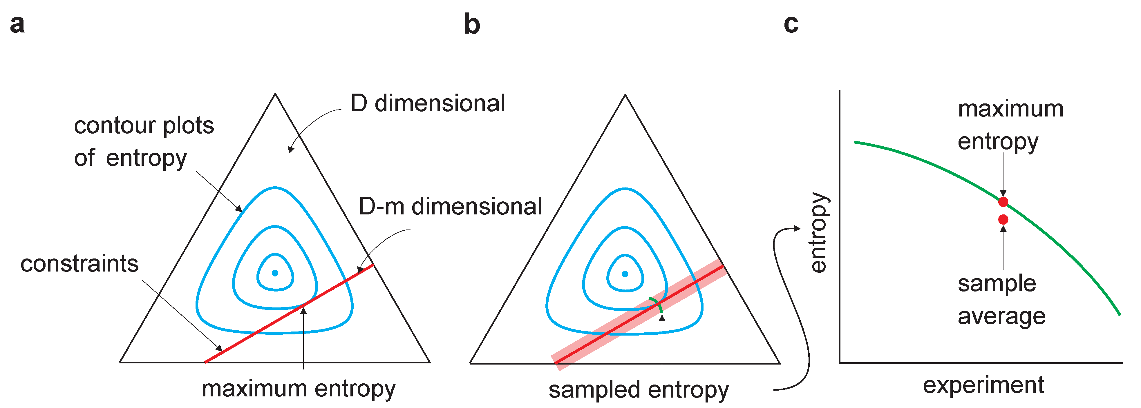
Figure 1. Sampling bias in maximum entropy models. The equilateral triangle represents a D-dimensional probability space (for the binary model considered here, $D=2^n-1$, where n is the dimensionality of $\mathbf{x}$). The cyan lines are contour plots of entropy; the red lines represent the m linear constraints and, thus, lie in a $D-m$ dimensional linear manifold. (a) Maximum entropy occurs at the tangential intersection of the constraints with the entropy contours. (b) The light red region indicates the range of constraints arising from multiple experiments in which a finite number of samples is drawn in each. Maximum entropy estimates from multiple experiments would lie along the green line. (c) As the entropy is concave, averaging the maximum entropy over experiments leads to an estimate that is lower than the true maximum entropy—estimating maximum entropy is subject to downward bias.

Figure 1. Sampling bias in maximum entropy models. The equilateral triangle represents a D-dimensional probability space (for the binary model considered here, $D=2^n-1$, where n is the dimensionality of $\mathbf{x}$). The cyan lines are contour plots of entropy; the red lines represent the m linear constraints and, thus, lie in a $D-m$ dimensional linear manifold. (a) Maximum entropy occurs at the tangential intersection of the constraints with the entropy contours. (b) The light red region indicates the range of constraints arising from multiple experiments in which a finite number of samples is drawn in each. Maximum entropy estimates from multiple experiments would lie along the green line. (c) As the entropy is concave, averaging the maximum entropy over experiments leads to an estimate that is lower than the true maximum entropy—estimating maximum entropy is subject to downward bias.

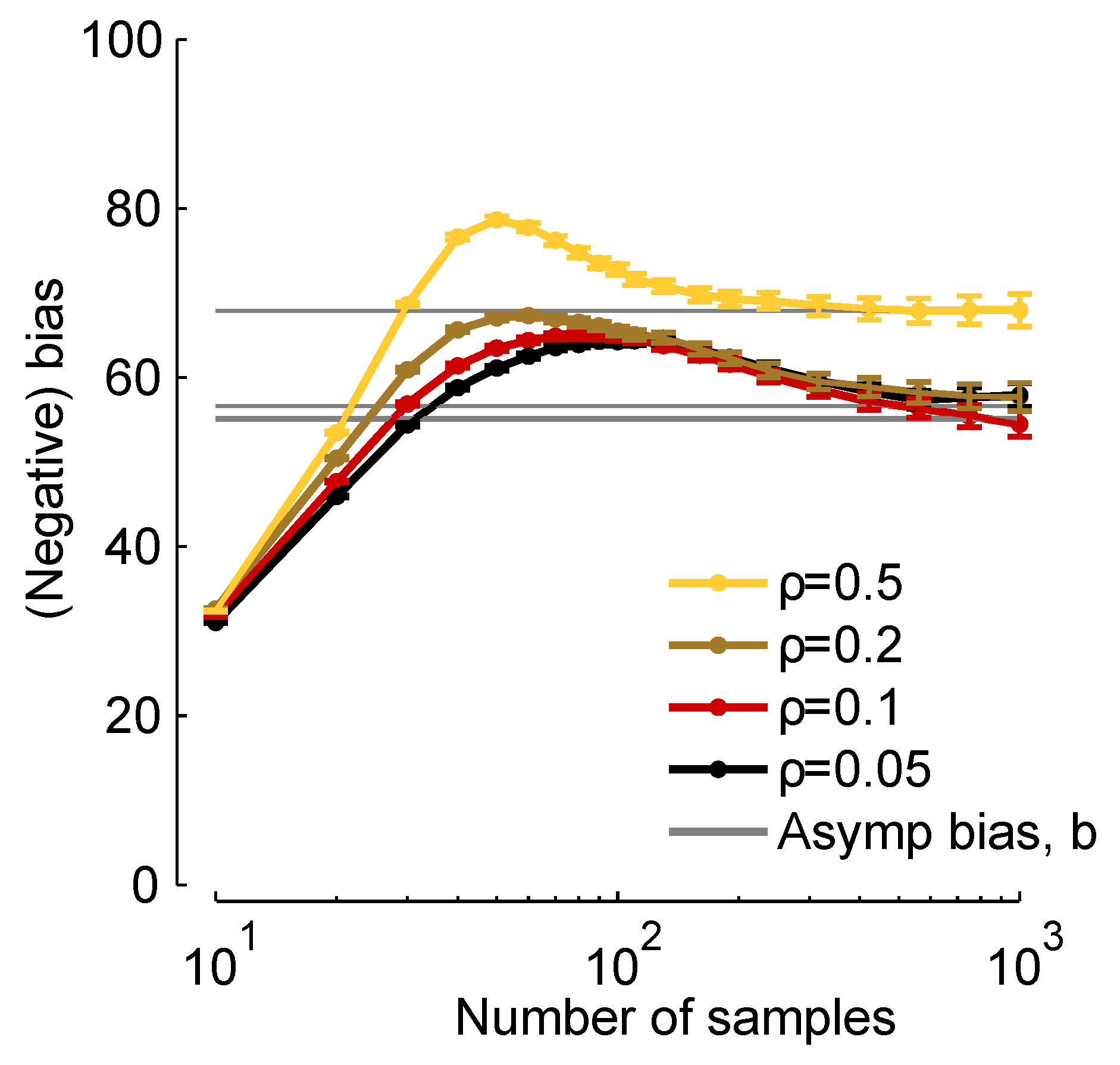
In Figure 2, we plot $-2K$ times the true bias ($-2K$ times the left-hand side of Equation (8), which we compute from finite samples), and b [via Equation (11)] versus the number of samples, K. When K is about 30, the two are close, and when $K>500$, they are virtually indistinguishable. Thus, although Equation (11) represents an approximation to the bias, it is a very good approximation for realistic data sets.

Figure 2. Normalized bias, b, versus number of samples, $\mathit{K}$. Grey lines: $\mathit{b}$, computed from Equation (11). Colored curves: $-\mathbf{2}\mathit{K}$ times the bias, computed numerically using the expression on the left-hand side of Equation (8). We used a homogeneous Dichotomized Gaussian distribution with $\mathit{n}=\mathbf{10}$ and a mean of 0.1. Different curves correspond to different correlation coefficients [see Equation (19) below], as indicated in the legend.

Figure 2. Normalized bias, b, versus number of samples, $\mathit{K}$. Grey lines: $\mathit{b}$, computed from Equation (11). Colored curves: $-\mathbf{2}\mathit{K}$ times the bias, computed numerically using the expression on the left-hand side of Equation (8). We used a homogeneous Dichotomized Gaussian distribution with $\mathit{n}=\mathbf{10}$ and a mean of 0.1. Different curves correspond to different correlation coefficients [see Equation (19) below], as indicated in the legend.

Evaluating the bias is, typically, hard. However, when the true distribution lies in the model class, so that $p\left(\mathbf{x}\right)=q\left(\mathbf{x}\right|\mathit{\mu })$, we can write down an explicit expression for it. That is because, in this case, ${\mathbf{C}}^q={\mathbf{C}}^p$, so the normalized bias [Equation (11)] is just the trace of the identity matrix, and we have $b=m$ (recall that m is the number of constraints); alternatively, the actual bias is $-m/2K$. An important within model-class case arises when the parametrized model is a histogram of the data. If $\mathbf{x}$ can take on M values, then there are $M-1$ parameters (the “$-1$” comes from the fact that $p\left(\mathbf{x}\right)$ must sum to one) and the bias is $-(M-1)/2K$. We thus recover a general version of the Miller-Madow [6] or Panzeri-Treves bias correction [7], which were derived for a multinomial distribution.

2.2. Is Bias Correction Important?

The fact that the bias falls off as $1/K$ means that we can correct for it simply by drawing a large number of samples. However, how large is “large”? For definitiveness, suppose we want to draw enough samples that the absolute value of the bias is less than ϵ times the true entropy, denoted $S_p$. Quantitatively, this means we want to choose K, so that $\left|\text{Bias}\right|<ϵS_p$. Using Equation (10) to relate the true bias to b, assuming that K is large enough that $-b/2K$ provides a good approximation to the true bias, and making use of the fact that b is positive, the condition $\left|\text{Bias}\right|<ϵS_p$ implies that K must be greater than $K_{min}$, where $K_{min}$ is given by:

$$\begin{array}{c}\hfill K_{min}=\frac{b}{2ϵS_p}\end{array}$$

(14)

Let us take $\mathbf{x}$ to be a vector with n components: $\mathbf{x}\equiv (x_1,x_2,...,x_n$). The average entropy of the components, denoted ${\overline{S}}_1$, is given by ${\overline{S}}_1=(1/n){\sum }_i{S}_p\left(x_i\right)$, where $S_p\left(x_i\right)$ is the true entropy of $x_i$. Since $n{\overline{S}}_1$, the “independent” entropy of $\mathbf{x}$, is greater than or equal to the true entropy, $S_p$, it follows that $K_{min}$ obeys the inequality:

$$\begin{array}{c}\hfill K_{min}\ge \frac{m}{2nϵ{\overline{S}}_1}\frac{b}{m}\end{array}$$

(15)

Not surprisingly, the minimum number of samples scales with the number of constraints, m (assuming $b/m$ does not have a strong m-dependence; something we show below). Often, m is at least quadratic in n; in that case, the minimum number of samples increases with the dimensionality of $\mathbf{x}$.

To obtain an explicit expression for m in terms of n, we consider a common class of maximum entropy models: second order models on binary variables. For these models, the functions $g_i\left(\mathbf{x}\right)$ constrain the mean and covariance of the $x_i$, so there are $m=n(n+1)/2$ parameters: n parameters for the mean and $n(n-1)/2$ for the covariance (because the $x_i$ are binary, the variances are functions of the means, which is why there are $n(n-1)/2$ parameters for the covariances rather than $n(n+1)/2$). Consequently, $m/n=(n+1)/2$ and, dropping the “$+1$” (which makes the inequality stronger), we have:

$$\begin{array}{c}\hfill K_{min}\ge \frac{n}{4ϵ{\overline{S}}_1}\frac{b}{m}\end{array}$$

(16)

How big is $K_{min}$ in practice? To answer that, we need estimates of ${\overline{S}}_1$ and $b/m$. Let us focus first on ${\overline{S}}_1$. For definiteness, here (and throughout the paper), we consider maximum entropy models that describe neural spike trains [15,16]. In that case, $x_i$ is one if there are one or more spikes in a time bin of size $\delta t$ and zero, otherwise. Assuming a population average firing rate of $\overline{\nu }$, and using the fact that entropy is concave, we have ${\overline{S}}_1\le h\left(\overline{\nu }\delta t\right)$, where $h\left(p\right)$ is the entropy of a Bernoulli variable with probability p: $h\left(p\right)=-plogp-(1-p)log(1-p)$. Using also the fact that $h\left(p\right)\le plog(e/p)$, we see that ${\overline{S}}_1\le \overline{\nu }\delta tlog(e/\left(\overline{\nu }\delta t\right))$, and so:

$$\begin{array}{c}\hfill K_{min}\ge \frac{n}{4ϵ\overline{\nu }\delta t}\frac{b/m}{log(e/\left(\overline{\nu }\delta t\right))}\end{array}$$

(17)

Exactly how to interpret $K_{min}$ depends on whether we are interested in the total entropy or the conditional entropy. For the total entropy, every data point is a sample, so the number of samples in an experiment that runs for time T is $T/\delta t$. The minimum time to run an experiment, denoted $T_{min}$, is, then, given by:

$$\begin{array}{c}\hfill T_{min}\ge \frac{n}{4ϵ\overline{\nu }}\frac{b/m}{log(e/\left(\overline{\nu }\delta t\right))}\end{array}$$

(18)

Ignoring for the moment the factor $b/m$ and the logarithmic term, the minimum experimental time scales as $n/4ϵ\overline{\nu }$. If one is willing to tolerate a bias of 10% of the true maximum entropy ($ϵ=0.1$) and the mean firing rate is not so low (say 10 Hz), then $T_{min}\sim n/4$ s. Unless n is in the hundreds of thousands, running experiments long enough to ensure an acceptably small bias is relatively easy. However, if the tolerance and firing rates drop, say to $ϵ=0.01$ and $\overline{\nu }=1$ Hz, respectively, then $T_{min}\sim 25n$ s, and experimental times are reasonable until n gets into the thousands. Such population sizes are not feasible with current technology, but they are likely to be in the not so distant future.

The situation is less favorable if one is interested in the mutual information. That is because to compute the mutual information, it is necessary to repeat the stimulus multiple times. Consequently, $K_{min}$ [Equation (17)] is the number of repeats, with the repeats typically lasting 1–10 s. Again, ignoring the factor $b/m$ and the logarithmic term, assuming, as above, that $ϵ=0.1$ and the mean firing rate is 10 Hz and taking the bin size to be (a rather typical) 10 ms, then $K_{min}\sim 25n$. For $n=10$, $K_{min}=250$, a number that is within experimental reach. When $n=100$; however, $K_{min}=2500$. For a one second stimulus, this is about 40 min, still easily within experimental reach. However, for a ten second stimulus, recording times approach seven hours, and experiments become much more demanding. Moreover, if the firing rate is 1 Hz and a tighter tolerance, say $ϵ=0.01$, is required, then $K_{min}=2500n$. Here, even if the stimulus lasts only one second, one must record for about 40 min per neuron—or almost seven hours for a population of 10 neurons. This would place severe constraints on experiments.

So far, we have ignored the factor $(b/m)/log(e/\left(\overline{\nu }\delta t\right))$ that appears in Equation (17) and Equation (18). Is this reasonable in practice, when the data is not necessarily well described by a maximum entropy model? We address this question in two ways: we compute it for a particular distribution, and we compute its maximum and minimum. The distribution we use is the Dichotomized Gaussian model [26,36], chosen because it is a good model of the higher-order correlations found in cortical recordings [27,29].

To access the large n regime, we consider a homogeneous model—one in which all neurons have the same firing rate, denoted ν, and all pairs have the same correlation coefficient, denoted ρ. In general, the correlation coefficient between neuron i and j is given by:

$$\begin{array}{c}\hfill {\rho }_{ij}\equiv \frac{\text{Covar}[x_i,x_j]}{{\left(\text{Var}\left[x_i\right]\text{Var}\left[x_j\right]\right)}^{1/2}}\end{array}$$

(19)

In the homogeneous model, all the ${\rho }_{ij}$ are the same and equal to ρ.

Assuming, as above, a bin size of $\delta t$, the two relevant parameters are the probability of firing in a bin, $\nu \delta t$, and the correlation coefficient, ρ. In Figure 3a,b, we plot $b/m$ (left axis) and $(b/m)/log(e/(\nu \delta t\left)\right)$ (right axis) versus n for a range of values for $\nu \delta t$ and ρ. There are two salient features to these plots. First, $b/m$ increases as $\nu \delta t$ decreases and as ρ increases, suggesting that bias correction is more difficult at low firing rates and high correlations. Second, the factor $(b/m)/log(e/(\nu \delta t\left)\right)$ that affects the minimum experimental time, $T_{min}$, has, for large n, a small range: a low of about 0.3 and a high of about one. Consequently, this factor has only a modest effect on the minimum number of trials one needs to avoid bias.

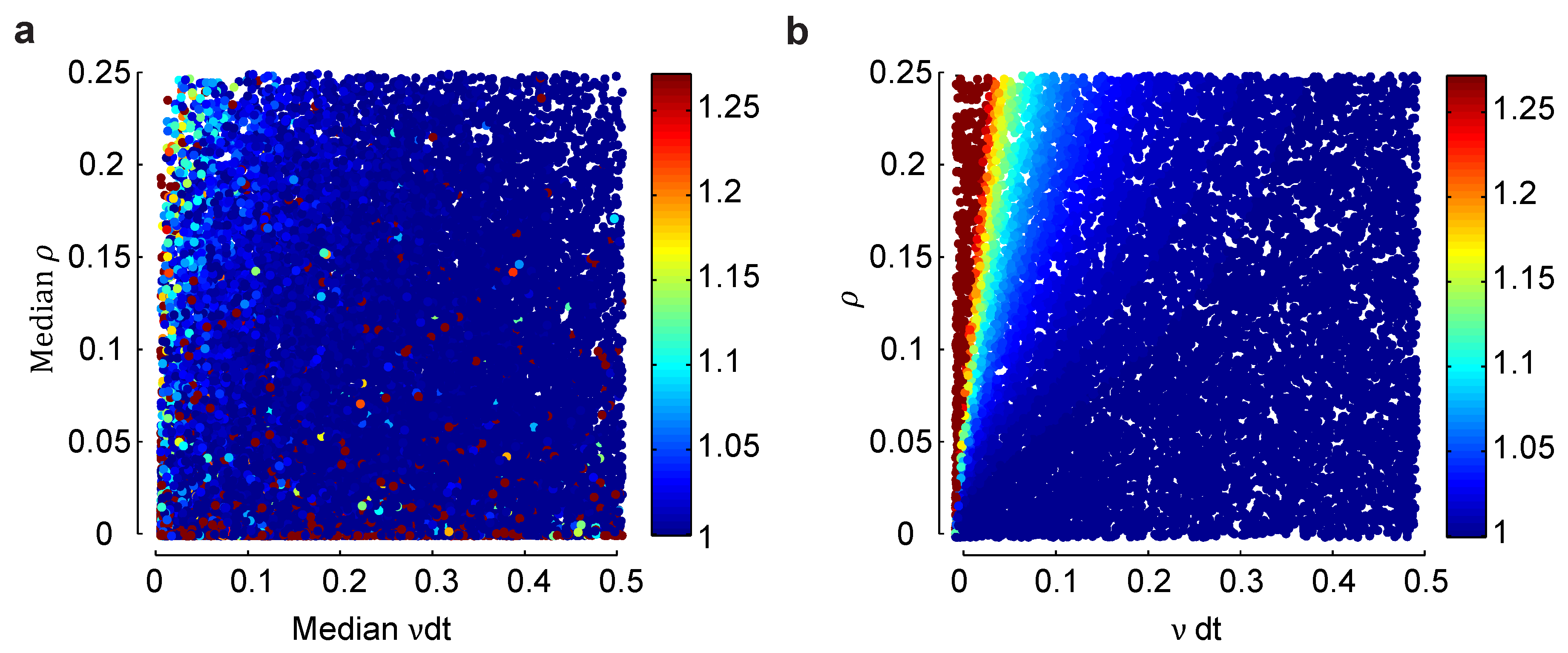
Figure 3 gives us $b/m$ for the homogeneous Dichotomized Gaussian model. Does the general picture—that $b/m$ is largest at low firing rates and high correlations, but never more than about four—hold for an inhomogeneous population, one in which different neurons have different firing rates and different pairs of neurons have different correlation coefficients? To address this question, in Figure 4, we compare a heterogeneous Dichotomized Gaussian model with $n=5$ neurons to a homogeneous model: in Figure 4a, we plot $b/m$ for a range of median firing rates and correlations coefficients in an inhomogeneous model, and in Figure 4b, we do the same for a homogeneous model. At very low firing rates, the homogeneous model is slightly more biased than the heterogeneous one, while at very low correlations, it is the other way around. Overall, though, the two models have very similar biases. Although not proof that the lack of difference will remain at large n, the results are at least not discouraging.

Figure 3. Scaling of the bias with population size for a homogeneous Dichotomized Gaussian model. (a) Bias, b, for $\nu \delta t=0.1$ and a range of correlation coefficients, ρ. The bias is biggest for strong correlations and large population sizes; (b) $\nu \delta t=0.02$ and a range of (smaller) correlation coefficients. In both panels, the left axis is $b/m$, and the right axis is $(b/m)/log(e/(\nu \delta t\left)\right)$. The latter quantity is important for determining the minimum number of trials [Equation (17)] or the minimum runtime [Equation (18)] needed to reduce bias to an acceptable level.

Figure 3. Scaling of the bias with population size for a homogeneous Dichotomized Gaussian model. (a) Bias, b, for $\nu \delta t=0.1$ and a range of correlation coefficients, ρ. The bias is biggest for strong correlations and large population sizes; (b) $\nu \delta t=0.02$ and a range of (smaller) correlation coefficients. In both panels, the left axis is $b/m$, and the right axis is $(b/m)/log(e/(\nu \delta t\left)\right)$. The latter quantity is important for determining the minimum number of trials [Equation (17)] or the minimum runtime [Equation (18)] needed to reduce bias to an acceptable level.

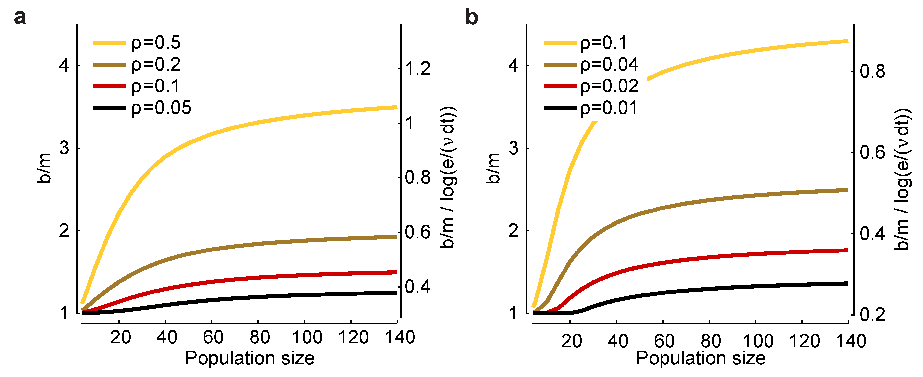
Figure 4. Effect of heterogeneity on the normalized bias in a small population. (a) Normalized bias relative to the within model class case, $b/m$, of a heterogeneous Dichotomized Gaussian model with $n=5$ as a function of the median mean, $\nu dt$, and correlation coefficient, ρ. As with the homogeneous model, bias is largest for small means and strong correlations. (b) The same plot, but for a homogeneous Dichotomized Gaussian. The difference in bias between the heterogeneous and homogeneous models is largest for small means and small correlations, but overall, the two plots are very similar.

Figure 4. Effect of heterogeneity on the normalized bias in a small population. (a) Normalized bias relative to the within model class case, $b/m$, of a heterogeneous Dichotomized Gaussian model with $n=5$ as a function of the median mean, $\nu dt$, and correlation coefficient, ρ. As with the homogeneous model, bias is largest for small means and strong correlations. (b) The same plot, but for a homogeneous Dichotomized Gaussian. The difference in bias between the heterogeneous and homogeneous models is largest for small means and small correlations, but overall, the two plots are very similar.

2.3. Maximum and Minimum Bias When the True Model is Not in the Model Class

Above, we saw that the factor $(b/m)/log(e/\left(\overline{\nu }\delta t\right))$ was about one for the Dichotomized Gaussian model. That is encouraging, but not definitive. In particular, we are left with the question: Is it possible for the bias to be much smaller or much larger than what we saw in Figure 3 and Figure 4? To answer that, we write the true distribution, $p\left(\mathbf{x}\right)$, in the form:

$$\begin{array}{c}\hfill p\left(\mathbf{x}\right)=q\left(\mathbf{x}\right|\mathit{\mu })+\delta p(\mathbf{x})\end{array}$$

(20)

and ask how the bias depends on $\delta p\left(\mathbf{x}\right)$; that is, how the bias changes as $p\left(\mathbf{x}\right)$ moves out of model class. To ensure that $\delta p\left(\mathbf{x}\right)$ represents only a move out of model class, and not a shift in the constraints (the ${\mu }_i$), we choose it, so that $p\left(\mathbf{x}\right)$ satisfies the same constraints as $q\left(\mathbf{x}\right|\mathit{\mu })$:

$$\begin{array}{c}\hfill \sum _{\mathbf{x}}p\left(\mathbf{x}\right)g_i\left(\mathbf{x}\right)=\sum _{\mathbf{x}}q\left(\mathbf{x}\right|\mathit{\mu })g_i\left(\mathbf{x}\right)={\mu }_i\end{array}$$

(21)

We cannot say anything definitive about the normalized bias in general, but what we can do is compute its maximum and minimum as a function of the distance between $p\left(\mathbf{x}\right)$ and $q\left(\mathbf{x}\right|\mathit{\mu })$. For “distance”, we use the Kullback–Leibler divergence, denoted $\Delta S$, which is given by:

$$\begin{array}{cc}\hfill \Delta S& =\sum _{\mathbf{x}}p\left(\mathbf{x}\right)log\frac{p\left(\mathbf{x}\right)}{q\left(\mathbf{x}\right|\mathit{\mu })}=S_q\left(\mathit{\mu }\right)-S_p\hfill \end{array}$$

(22)

where $S_p$ is the entropy of $p\left(\mathbf{x}\right)$. The second equality follows from the definition of $q\left(\mathbf{x}\right|\mathit{\mu })$, Equation (4) and the fact that ${\langle g_i\left(\mathbf{x}\right)\rangle }_{p\left(\mathbf{x}\right)}={\langle g_i\left(\mathbf{x}\right)\rangle }_{q\left(\mathbf{x}\right|\mu \mathit{)}}$, which comes from Equation (21).

Rather than maximizing the normalized bias at fixed $\Delta S$, we take a complementary approach and minimize $\Delta S$ at fixed bias. Since $S_q\left(\mathit{\mu }\right)$ is independent of $p\left(\mathbf{x}\right)$, minimizing $\Delta S$ is equivalent to maximizing $S_p$ (see Equation (22)). Thus, again, we have a maximum entropy problem. Now, though, we have an additional constraint on the normalized bias. To determine exactly what that constraint is, we use Equation (11) and (12) to write:

$$\begin{array}{c}\hfill b={\langle B\left(\mathbf{x}\right)\rangle }_{p\left(\mathbf{x}\right)}\end{array}$$

(23)

where:

$$\begin{array}{c}\hfill B\left(\mathbf{x}\right)\equiv \sum _{ij}\delta g_i\left(\mathbf{x}\right)C_{ij}^{q^{-1}}\delta g_j\left(\mathbf{x}\right)\end{array}$$

(24)

and, importantly, $C_{ij}^q$ depends on $q(\mathbf{x},\mathit{\mu })$, but not on $\delta p\left(\mathbf{x}\right)$ [see Equation (12a)]. Fixed normalized bias, b, thus corresponds to fixed ${\langle B\left(\mathbf{x}\right)\rangle }_{p\left(\mathbf{x}\right)}$. This additional constraint introduces an additional Lagrange multiplier besides the ${\lambda }_i$, which we denote β. Taking into account the additional constraint, and using the same analysis that led to Equation (4), we find that the distribution with the smallest difference in entropy, $\Delta S$, at fixed b, which we denote $q\left(\mathbf{x}\right|\mathit{\mu },\beta )$, is given by:

$$\begin{array}{c}\hfill q\left(\mathbf{x}\right|\mathit{\mu },\beta )=\frac{exp\left[\beta B\left(\mathbf{x}\right)+{\sum }_i{\lambda }_i(\mathit{\mu },\beta )g_i\left(\mathbf{x}\right)\right]}{Z(\mathit{\mu },\beta )}\end{array}$$

(25)

where $Z(\mathit{\mu },\beta )$ is the partition function, the ${\lambda }_i(\mathit{\mu },\beta )$ are chosen to satisfy Equation (7), but with $p\left(\mathbf{x}\right)$ replaced by $q\left(\mathbf{x}\right|\mathit{\mu },\beta )$, and β is chosen to satisfy Equation (23), but with, again, $p\left(\mathbf{x}\right)$ replaced by $q\left(\mathbf{x}\right|\mathit{\mu },\beta )$. Note that we have slightly abused notation; whereas, in the previous sections, ${\lambda }_i$ and Z depended only on μ, now they depend on both μ and β. However, the previous variables are closely related to the new ones: when $\beta =0$, the constraint associated with b disappears, and we recover $q\left(\mathbf{x}\right|\mu )$; that is, $q\left(\mathbf{x}\right|\mathit{\mu },0)=q(\mathbf{x}\left|\mathit{\mu }\right)$. Consequently, ${\lambda }_i(\mathit{\mu },0)={\lambda }_i\left(\mathit{\mu }\right)$, and $Z(\mathit{\mu },0)=Z\left(\mathit{\mu }\right)$.

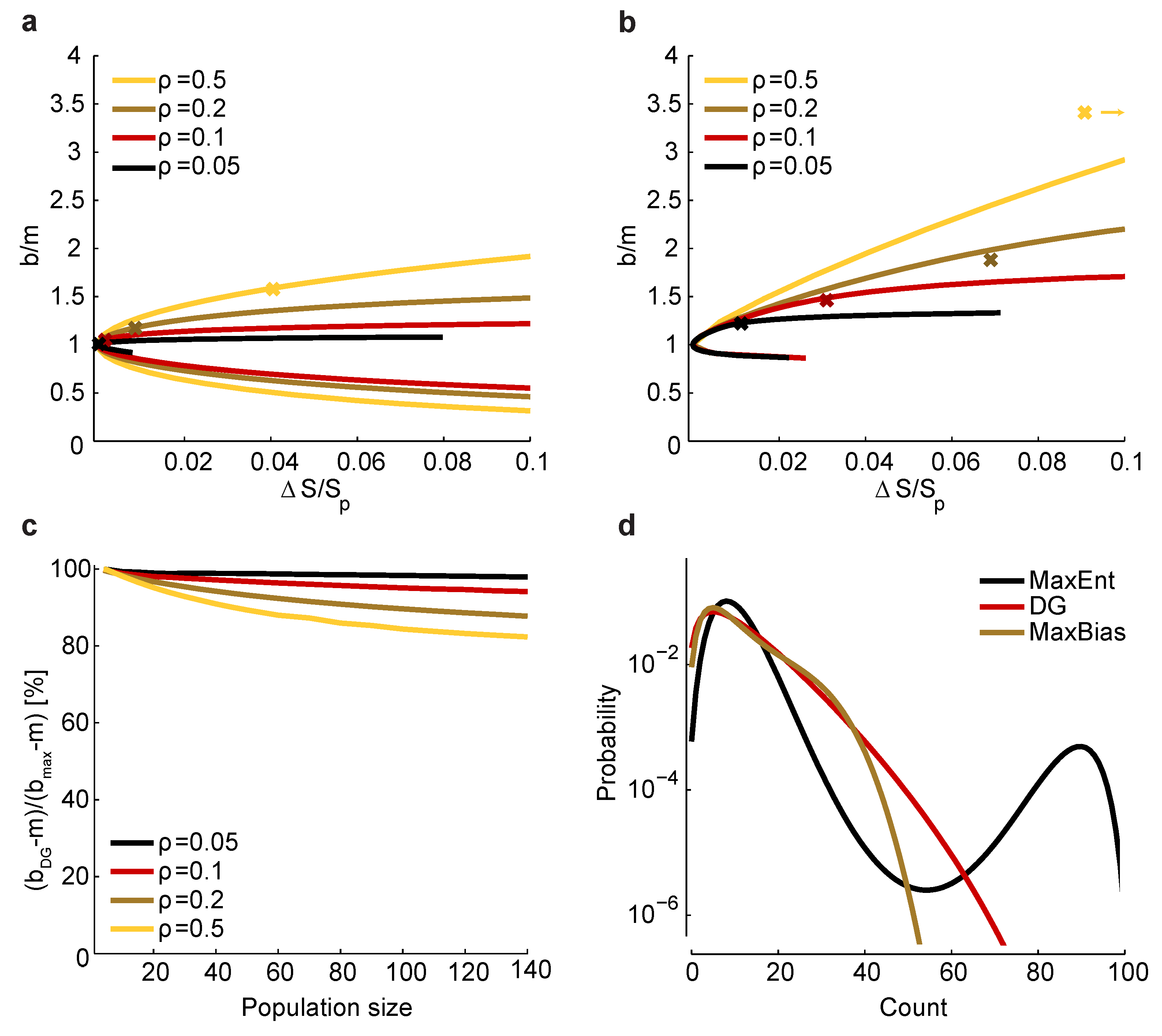
Figure 5. Relationship between $\Delta S$ and bias. (a) Maximum and minimum normalized bias relative to m versus $\Delta S/S_p$ (recall that $S_p$ is the entropy of $p\left(\mathbf{x}\right)$) in a homogeneous population with size $n=5$, $\nu \delta t=0.1$, and correlation coefficients indicated by color. The crosses correspond to a set of homogeneous Dichotomized Gaussian models with $\nu \delta t=0.1$. (b) Same as a, but for $n=100$. For $\rho =0.5$, the bias of the Dichotomized Gaussian model is off the right-hand side of the plot, at $(0.17,3.4)$; for comparison, the maximum bias at $\rho =0.5$ and $\Delta S/S_p=0.17$ is 3.8. (c) Comparison between the normalized bias of the Dichotomized Gaussian model and the maximum normalized bias. As in panels a and b, we used $\nu \delta t=0.1$. Because the ratio of the biases is trivially near one when b is near m, we plot $(b_{DG}-m)/(b_{max}-m)$, where $b_{DG}$ and $b_{max}$ are the normalized bias of the Dichotomized Gaussian and the maximum bias, respectively; this is the ratio of the “additional” bias. (d) Distribution of total spike count ($={\sum }_i{x}_i$) for the Dichotomized Gaussian, maximum entropy (MaxEnt) and maximally biased (MaxBias) models with $n=100$, $\nu \delta t=0.1$ and $\rho =0.05$. The similarity between the distributions of the Dichotomized Gaussian and maximally biased models is consistent with the similarity in normalized biases shown in panel c.

Figure 5. Relationship between $\Delta S$ and bias. (a) Maximum and minimum normalized bias relative to m versus $\Delta S/S_p$ (recall that $S_p$ is the entropy of $p\left(\mathbf{x}\right)$) in a homogeneous population with size $n=5$, $\nu \delta t=0.1$, and correlation coefficients indicated by color. The crosses correspond to a set of homogeneous Dichotomized Gaussian models with $\nu \delta t=0.1$. (b) Same as a, but for $n=100$. For $\rho =0.5$, the bias of the Dichotomized Gaussian model is off the right-hand side of the plot, at $(0.17,3.4)$; for comparison, the maximum bias at $\rho =0.5$ and $\Delta S/S_p=0.17$ is 3.8. (c) Comparison between the normalized bias of the Dichotomized Gaussian model and the maximum normalized bias. As in panels a and b, we used $\nu \delta t=0.1$. Because the ratio of the biases is trivially near one when b is near m, we plot $(b_{DG}-m)/(b_{max}-m)$, where $b_{DG}$ and $b_{max}$ are the normalized bias of the Dichotomized Gaussian and the maximum bias, respectively; this is the ratio of the “additional” bias. (d) Distribution of total spike count ($={\sum }_i{x}_i$) for the Dichotomized Gaussian, maximum entropy (MaxEnt) and maximally biased (MaxBias) models with $n=100$, $\nu \delta t=0.1$ and $\rho =0.05$. The similarity between the distributions of the Dichotomized Gaussian and maximally biased models is consistent with the similarity in normalized biases shown in panel c.

The procedure for determining the relationship between $\Delta S$ and the normalized bias, b, involves two steps: first, for a particular bias, b, choose the ${\lambda }_i$ and β in Equation (25) to satisfy the constraints given in Equation (2) and the condition ${\langle B\left(x\right)\rangle }_{q\left(\mathbf{x}\right|\mu ,\mathit{\beta })}=b$; second, compute $\Delta S$ from Equation (22). Repeating those steps for a large number of biases will produce curves like the ones shown in Figure 5a,b.

Since the true entropy, $S_p$, is maximized (subject to constraints) when $\beta =0$, it follows that $\Delta S$ is zero when $\beta =0$ and nonzero, otherwise. In fact, in the Methods, we show that $\Delta S$ has a single global minimum at $\beta =0$; we also show that the normalized bias, b, is a monotonic increasing function of β. Consequently, there are two normalized biases that have the same $\Delta S$, one larger than m and the other smaller. This is shown in Figure 5a,b, where we plot $b/m$ versus $\Delta S/S_p$ for the homogeneous Dichotomized Gaussian model. It turns out that this model has near maximum normalized bias, as shown in Figure 5c. Consistent with that, the Dichotomized Gaussian model has about the same distribution of spike counts as the maximally biased models, but a very different distribution from the maximum entropy model (Figure 5d).

The fact that the Dichotomized Gaussian model has near maximum normalized bias is important, because it tells us that the bias we found in Figure 3 and Figure 4 is about as large as one could expect. In those figures, we found that $b/m$ had a relatively small range—from about one to four. Although too large to be used for bias correction, this range is small enough that one could use it to get a conservative estimate of the minimum number of trials [Equation (17)] or minimum run time [Equation (18)] it would take to reduce bias to an acceptable level.

2.4. Using a Plug-in Estimator to Reduce Bias

Given that we have an expression for the asymptotic normalized bias, b [Equation (11)], it is, in principle, possible to correct for it (assuming that K is large enough for the asymptotic bias to be valid). If the effect of model-misspecification is negligible (which is typically the case if the neurons are sufficiently weakly correlated), then the normalized bias is just m, the number of constraints, and bias correction is easy: simply subtract $m/2K$ from our estimate of the entropy. If, however, there is substantial model-misspecification, we need to estimate covariance matrices under the true and maximum entropy models. Of course, these estimates are subject to their own bias, but we can ignore that and use a “plug-in” estimator; an estimator computed from the covariance matrices in Equation (11), ${\mathbf{C}}^p$ and ${\mathbf{C}}^q$, which, in turn, are computed from data. Specifically, we estimate ${\mathbf{C}}^p$ and ${\mathbf{C}}^q$ using:

$$\begin{array}{cc}\hfill {\widehat{C}}_{ij}^q& =\sum _{\mathbf{x}}q\left(\mathbf{x}\right|\widehat{\mathit{\mu }})\delta g_i\left(\mathbf{x}\right)\delta g_j\left(\mathbf{x}\right)\hfill \end{array}$$

(26a)

$$\begin{array}{cc}\hfill {\widehat{C}}_{ij}^p& =\frac{1}{K}\sum _{k=1}^K\delta g_i\left({\mathbf{x}}^{\left(k\right)}\right)\delta g_j\left({\mathbf{x}}^{\left(k\right)}\right)\hfill \end{array}$$

(26b)

Such an estimator is plotted in Figure 6a for a homogeneous Dichotomized Gaussian with $n=10$ and $\nu \delta t=0.1$. Although the plug-in estimator converges to the correct value for sample sizes above about 500, it underestimates b by a large amount, even when $K\sim 100$. To reduce this effect, we considered a thresholded estimator, denoted $b_{\text{thresh}}$, which is given by:

$$\begin{array}{c}\hfill b_{\text{thresh}}\equiv max(b_{\text{plugin}},m)\end{array}$$

(27)

where $b_{\text{plugin}}$ comes from Equation (11). This estimator is motivated by the fact that we found, empirically, that the additional bias due to model misspecification was almost always greater than m.

Figure 6. Bias correction. (a) Plug-in, $b_{\text{plugin}}$, and thresholded, $b_{\text{thresh}}$, estimators versus sample size for a homogeneous Dichotomized Gaussian model with $n=10$ and $\nu \delta t=0.1$. Correlations are color coded as in Figure 5. Gray lines indicate the true normalized bias as a function of sample size, computed numerically as for Figure 2. (b) Relative error without bias correction, $(S_q\left(\widehat{\mathit{\mu }}\right)-S_q\left(\mathit{\mu }\right))/S_q\left(\mathit{\mu }\right)$, with the plug-in correction, $(S_q\left(\widehat{\mathit{\mu }}\right)+2K{b}_{\text{plugin}}-S_q\left(\mathit{\mu }\right))/S_q\left(\mathit{\mu }\right)$, and with the thresholded estimator, $(S_q\left(\widehat{\mathit{\mu }}\right)+2K{b}_{\text{thresh}}-S_q\left(\mathit{\mu }\right))/S_q\left(\mathit{\mu }\right)$.

Figure 6. Bias correction. (a) Plug-in, $b_{\text{plugin}}$, and thresholded, $b_{\text{thresh}}$, estimators versus sample size for a homogeneous Dichotomized Gaussian model with $n=10$ and $\nu \delta t=0.1$. Correlations are color coded as in Figure 5. Gray lines indicate the true normalized bias as a function of sample size, computed numerically as for Figure 2. (b) Relative error without bias correction, $(S_q\left(\widehat{\mathit{\mu }}\right)-S_q\left(\mathit{\mu }\right))/S_q\left(\mathit{\mu }\right)$, with the plug-in correction, $(S_q\left(\widehat{\mathit{\mu }}\right)+2K{b}_{\text{plugin}}-S_q\left(\mathit{\mu }\right))/S_q\left(\mathit{\mu }\right)$, and with the thresholded estimator, $(S_q\left(\widehat{\mathit{\mu }}\right)+2K{b}_{\text{thresh}}-S_q\left(\mathit{\mu }\right))/S_q\left(\mathit{\mu }\right)$.

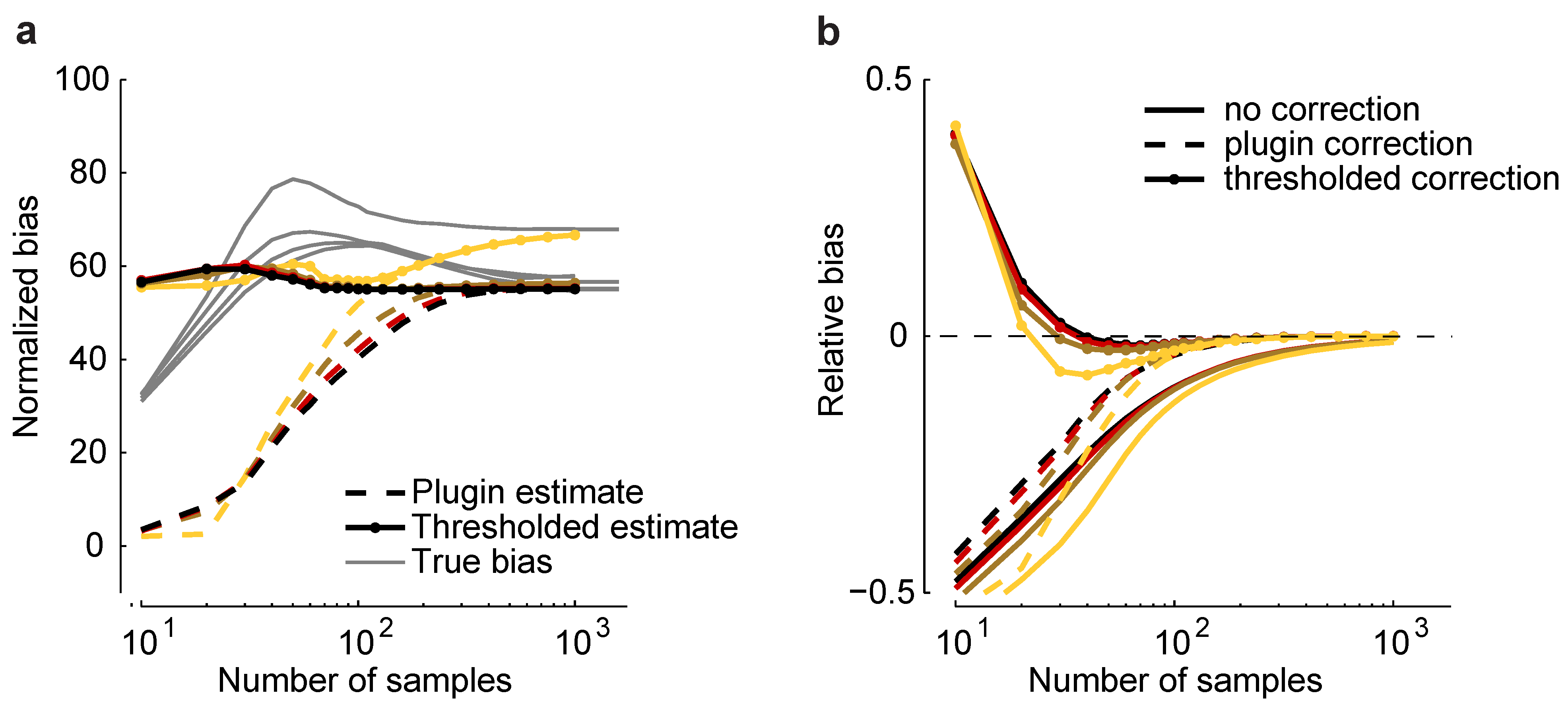
As shown in Figure 6a, $b_{\text{thresh}}$ is closer to the true normalized bias than $b_{\text{plugin}}$. In Figure 6b, we plot the relative error of the uncorrected estimate of the maximum entropy, $\left(S_q\left(\widehat{\mathit{\mu }}\right)-S_q\left(\mathit{\mu }\right)\right)/S_q\left(\mathit{\mu }\right)$, and the same quantity, but with two corrections: the plug-in correction, $\left(S_q\left(\widehat{\mathit{\mu }}\right)+2K{b}_{\text{plugin}}-S_q\left(\mathit{\mu }\right)\right)/S_q\left(\mathit{\mu }\right)$, and the thresholded correction, $\left(S_q\left(\widehat{\mathit{\mu }}\right)+2K{b}_{\text{thresh}}-S_q\left(\mathit{\mu }\right)\right)/S_q\left(\mathit{\mu }\right)$. Using the plug-in estimator, accurate estimates of the maximum entropy can be achieved with about 100 samples; using the threshold estimators, as few as 30 samples are needed. This suggests that our formalism can be used to perform bias correction for maximum entropy models, even in the presence of model-misspecification.

3. Discussion

In recent years, there has been a resurgence of interest in maximum entropy models, both in neuroscience [13,15,16,18,19,20,21,22] and in related fields [23,24,25]. In neuroscience, these models have been used to estimate entropy. Although maximum entropy based estimators do much better than brute-force estimators, especially when multiple neurons are involved, they are still subject to bias. In this paper, we studied, both analytically and through simulations, just how big the bias is. We focused on the commonly used “naive” estimator, i.e., an estimator of the entropy, which is calculated directly from the empirical estimates of the probabilities of the model.

Our main result is that we found a simple expression for the bias in terms of covariance matrices under the true and maximum entropy distributions. Based on this, we showed that if the true model is in the model class, the (downward) bias in the estimate of the maximum entropy is proportional to the ratio of the number of parameters to the number of observations, a relationship that is identical to that of naive histogram estimators [6,7]. This bias grows quadratically with population size for second-order binary maximum entropy models (also known as Ising models).

What happens when the model is misspecified; that is, when the true data does not come from a maximum entropy distribution? We investigated this question for, again, second-order binary maximum entropy models. We found that model misspecification generally increases bias, but the increase is modest—for a population of 100 neurons and strong correlations ($\rho =0.1$), model misspecification increased bias by a factor of at most four (see Figure 3b). Experimentally, correlation coefficients are usually substantially below 0.1 [15,16,18,20], so a conservative estimate of the minimum number of samples one needs in an experiment can be obtained from Equation (17) with $b/m=4$. However, this estimate assumes that our results for homogeneous populations apply to heterogeneous populations, something we showed only for relatively small populations (five neurons).

Has bias been a problem in experiments so far? The answer is largely no. Many of the experimental studies focused on the total entropy, using either no more than 10 neurons [15,16,18,20] or using populations as large as 100, but with a heavily regularized model [17]. In both cases, recordings were sufficiently long that bias was not an issue. There have been several studies that computed mutual information, which generally takes more data than entropy [19,37,38,39]. Two were very well sampled: Ohiorhenuan et al. [19] used about 30,000 trials per stimulus, and Granot-Atedgi et al. [39] used effectively 720,000 trials per stimulus (primarily because they used the whole data set to compute the pairwise interactions). Two other studies, which used a data set with an average of about 700 samples per trial [40], were slightly less well sampled. The first used a homogeneous model (the firing rates and all higher order correlations were assumed to be neuron-independent) [37]. This reduced the number of constraints, m, to at most five. Since there were about 700 trials per stimulus, the approximate downward bias, $m/2K$ with $K=700$, was 0.004 bits. This was a factor of 125 smaller than the information in the population, which was on the order of 0.5 bits, so the maximum error due to bias would have been less than 1%. The other study, based on the same data, considered a third order maximum entropy model and up to eight units [38]. For such a model, the number of constraints, m, is $n(n^2+5)/6$ (=$n+n(n-1)/2+n(n-1)(n-2)/6$). Consequently, the approximate downward bias was $n(n^2+5)/12K$. With $n=8$ and $K=700$, the bias is 0.07 bits. This is more than 10% of information, which was about 0.6 bits. However, the authors applied a sophisticated bias correction to the mutual information [38] and checked to see that splitting the data in half did not change the information, so their estimates are likely to be correct. Nevertheless, this illustrates that bias in maximum entropy models can be important, even with current data sets. Furthermore, given the exponential rate at which recorded population sizes are growing [41], bias is likely to become an increasingly major concern.

Because we could estimate bias, via Equation (10) and Equation (11), we could use that estimate to correct for it. Of course, any correction comes with further estimation problems: in the case of model misspecification, the bias has to be estimated from data, so it too may be biased; even if not, it could introduce additional variance. This is, potentially, especially problematic for our bias correction, as it depends on two covariance matrices, one of which has to be inverted. Nevertheless, in the interests of simplicity, we used a plug-in estimator of the bias (with a minor correction associated with matrix singularities). In spite of the potential drawbacks of our simple estimator (including the fact that it assumes Equation (11) is valid even for very small sample sizes, K), it worked well: for the models we studied, it reduced the required number of samples by a factor of about three—from 100 to about 30. While this is a modest reduction, it could be important in electrophysiological experiments, where it is often difficult to achieve long recording times. Furthermore, it is likely that it could be improved: more sophisticated estimation techniques, such as modified entropy estimates [5], techniques for bias-reduction for mutual information [8,42] or Bayesian priors [30,31,43], could provide additional or more effective bias reduction.

4. Methods

4.1. Numerical Methods

For all of our analysis, we use the Dichotomized Gaussian distribution [26,27,36], a distribution over binary variables, $\mathbf{x}=(x_1,x_2,...,x_n)$, where $x_i$ can take on the values, 0 or 1. The distribution can be defined by a sampling procedure: first, sample a vector, $\mathbf{z}$, from a Gaussian distribution with mean γ and covariance Λ:

$$\begin{array}{c}\hfill \mathbf{z}\sim \mathcal{N}(\gamma ,\Lambda )\end{array}$$

(28)

then, set $x_i$ to $+1$ if $z_i>0$ and 0, otherwise. Alternatively, we may write:

$$\begin{array}{c}\hfill p(x_1,x_2,...,x_n)=p((2x_1-1)z_1>0,(2x_2-1)z_2>0,...,(2x_n-1)z_n>0)\end{array}$$

(29)

where $p\left(\mathbf{z}\right)$ is given by Equation (28).

Given this distribution, our first step is to sample from it and, then, using those samples, fit a pairwise maximum entropy model. More concretely, for any mean and covariance, γ and Λ, we generate samples (${\mathbf{x}}^{\left(k\right)}$, $k=1,...,K$); from those, we compute the ${\widehat{\mu }}_i$ [Equation (1)]; and from the ${\widehat{\mu }}_i$, we compute the parameters of the maximum entropy model, ${\lambda }_i$ [Equation (4)]. Once we have those parameters, we can compute the normalized bias via Equation (11).

While this is straightforward in principle, it quickly becomes unwieldy as the number of neurons increases (scaling is exponential in n). Therefore, to access the large n regime, we use the homogeneous Dichotomized Gaussian distribution, for which all the means, variances and covariances are the same: ${\gamma }_i=\gamma$ and ${\Lambda }_{ij}={\sigma }^2{\delta }_{ij}+{\sigma }^2\rho (1-{\delta }_{ij})$. The symmetries of this model make it possible to compute all quantities of interest (entropy of the Dichotomized Gaussian distribution model, entropy of the maximum entropy model, normalized bias via Equation (11) and minimum and maximum normalized bias given distance from the model class) without the need for numerical approximations [27].

4.1.1. Parameters of the Heterogeneous Dichotomized Gaussian Distribution

For the heterogeneous Dichotomized Gaussian distribution, we need to specify γ and Λ. Both were sampled from random distributions. The mean, ${\gamma }_i$, came from a zero mean, unit variance Gaussian distribution, but truncated at zero, so that only negative ${\gamma }_i$s were generated. We used negative ${\gamma }_i$s, because for neural data, the probability of not observing a spike (i.e. $x_i=0$) is generally larger than that of observing a spike (i.e. $x_i=1$). Generation of the covariance matrix, Λ, was more complicated and proceeded in several steps. The first was to construct a covariance matrix corresponding to a homogeneous population model; that is, a covariance matrix with 1 along the diagonal and ρ an all the off-diagonal elements. The next step was to take the Cholesky decomposition of the homogeneous matrix; this resulted in a matrix, $\mathbf{G}$, with zeros in the upper triangular entries. We then added Gaussian noise to the lower-triangular entries of $\mathbf{G}$ (the non-zero entries). Finally, the last step was to set Λ to $(\mathbf{G}+\mathbf{N})·{(\mathbf{G}+\mathbf{N})}^{\top }$, where $\mathbf{N}$ is the noise added to the lower-triangular entries and ⊤ denotes the transpose. Because we wanted covariance matrices with a range of median correlation coefficients, the value of ρ was sampled uniformly from the range, $[0.0,0.8]$. Similarly, to get models that ranged from weakly to strongly heterogeneous, the standard deviation of the noise we added to the Cholesky-decomposition was sampled uniformly from {0.1, 0.25, 0.5, 1, 2}.

4.1.2. Fitting Maximum Entropy Models

To find the parameters of the maximum entropy models (the ${\lambda }_i$), we numerically maximized the log-likelihood using a quasi-Newton implementation [44]. The log likelihood, denoted $\mathcal{L}$, is given by:

$$\begin{array}{c}\hfill \mathcal{L}=\frac{1}{K}\sum _{k=1}^{K}logq\left({\mathbf{x}}^{\left(k\right)}\right|\widehat{\mathit{\mu }})=\frac{1}{K}\sum _{k=1}^K\sum _{i=1}^m{\lambda }_i\left(\widehat{\mathit{\mu }}\right)g_i\left({\mathbf{x}}^{\left(k\right)}\right)-logZ\left(\widehat{\mathit{\mu }}\right)\end{array}$$

(30)

with the second equality following from Equation (4). Optimization was stopped when successive iterations increased the log-likelihood by less than ${10}^{-20}$. This generally led to a model for which all moments were within ${10}^{-8}$ of the desired empirical moments.

4.1.3. Bias Correction

To compute the normalized bias, b [Equation (11)], we first estimate the covariance matrices under the true and maximum entropy distributions via Equation (26); these are denoted ${\widehat{\mathbf{C}}}^p$ and ${\widehat{\mathbf{C}}}^q$, respectively. We then have to invert ${\widehat{\mathbf{C}}}^q$. However, given finite data, there is no guarantee that ${\widehat{\mathbf{C}}}^q$ will be full rank. For example, if two neurons have low firing rates, synchronous spikes occur very infrequently, and the empirical estimate of $\langle x_i{x}_j\rangle$ can be zero for some i and j; say $i_0$ and $j_0$. In this case, the corresponding λ will be infinity [see Equation (4)]; and so, ${\widehat{C}}_{i^{\prime }{j}^{\prime },i_0{j}_0}^q$ will be zero for all $(i^{\prime },j^{\prime })$ pairs, and ${\widehat{C}}_{i^{\prime },i_0{j}_0}^q$ will be zero for all $i^{\prime }$. In other words, ${\widehat{\mathbf{C}}}^q$ will have a row and column of zeros (and if the estimate of $\langle x_i{x}_j\rangle$ is zero for several $(i,j)$ pairs, there will be several rows and columns of zeros). The corresponding rows and columns of ${\widehat{\mathbf{C}}}^p$ will also be zero, making $b_{\text{plugin}}(=\text{tr}[{{\mathbf{C}}^q}^{-1}·{\mathbf{C}}^p])$ well behaved in principle. In practice, however, this quantity is not well behaved, and $b_{\text{plugin}}$ will, in most cases, be close to $m-m_0$, where $m_0$ is the number of all-zero rows and columns. In some cases, however, $b_{\text{plugin}}$ took on very large values (or was not defined). We attribute these cases to numerical problems arising from the inversion of the covariance matrix. We therefore rejected any data sets for which $b_{\text{plugin}}>10m$. It is likely that this problem could be fixed with a more sophisticated (e.g., Bayesian) estimator of empirical averages, or by simply dropping the rows and columns that are zero, computing $b_{\text{plugin}}$, and then adding back in the number of dropped rows.

4.1.4. Sample Size

When estimating entropy for a particular model (a particular value of γ and Λ), for each K we averaged over $10,000$ data sets. Error bars denote the standard error of the mean across data sets.

4.2. The Normalized Bias Depends Only on the Covariance Matrices

The normalized bias, b, given in Equation (10), depends on two quantities: ${\partial }^2{S}_q\left(\mathit{\mu }\right)/\partial {\mu }_i\partial {\mu }_j$ and $\langle \delta {\mu }_i\delta {\mu }_j\rangle$. Here, we derive explicit expressions for both. The second is the easier of the two: noting that $\delta {\mu }_i$ is the mean of K uncorrelated, zero mean random variables [see Equation (9)], we see that:

$$\begin{array}{c}\hfill \langle \delta {\mu }_i\delta {\mu }_j\rangle =\frac{1}{K}\left[{\langle g_i\left(\mathbf{x}\right)g_j\left(\mathbf{x}\right)\rangle }_{p\left(\mathbf{x}\right)}-{\langle g_i\left(\mathbf{x}\right)\rangle }_{p\left(\mathbf{x}\right)}{\langle g_j\left(\mathbf{x}\right)\rangle }_{p\left(\mathbf{x}\right)}\right]=\frac{C_{ij}^p}{K}\end{array}$$

(31)

where the last equality follows from the definition given in Equation (12a).

For the first, we have:

$$\begin{array}{c}\hfill \frac{\partial {}^2{S}_q\left(\mathit{\mu }\right)}{\partial {\mu }_i\partial {\mu }_j}=\frac{\partial }{\partial {\mu }_i}\left[\frac{\partial logZ\left(\mathit{\mu }\right)}{\partial {\mu }_j}-{\lambda }_j-\sum _l{\mu }_l\frac{\partial {\lambda }_l}{\partial {\mu }_j}\right]\end{array}$$

(32)

where we used Equation (6) for the entropy. From the definition of $Z\left(\mathit{\mu }\right)$, Equation (5), it is straightforward to show that

$$\begin{array}{c}\hfill \frac{\partial logZ\left(\mathit{\mu }\right)}{\partial {\mu }_j}=\sum _l{\mu }_l\frac{\partial {\lambda }_l}{\partial {\mu }_j}\end{array}$$

(33)

Inserting Equation (33) into Equation (32), the first and third terms cancel, and we are left with:

$$\begin{array}{c}\hfill \frac{\partial {}^2{S}_q\left(\mathit{\mu }\right)}{\partial {\mu }_i\partial {\mu }_j}=-\frac{\partial {\lambda }_j}{\partial {\mu }_i}\end{array}$$

(34)

This quantity is hard to compute directly, so instead, we compute its inverse, $\partial {\mu }_i/\partial {\lambda }_j$. Using the definition of ${\mu }_i$:

$$\begin{array}{c}\hfill {\mu }_i=\sum _{\mathbf{x}}{g}_i\left(\mathbf{x}\right)\frac{exp\left[{\sum }_j{\lambda }_j{g}_j\left(\mathbf{x}\right)\right]}{Z\left(\mathit{\mu }\right)}\end{array}$$

(35)

differentiating both sides with respect to ${\lambda }_j$ and applying Equation (33), we find that:

$$\begin{array}{c}\hfill \frac{\partial {\mu }_i}{\partial {\lambda }_j}={\langle g_j\left(\mathbf{x}\right)g_i\left(\mathbf{x}\right)\rangle }_{q\left(\mathbf{x}\right|\mathit{\mu })}-{\langle g_j\left(\mathbf{x}\right)\rangle }_{q\left(\mathbf{x}\right|\mathit{\mu })}{\langle g_i\left(\mathbf{x}\right)\rangle }_{q\left(\mathbf{x}\right|\mathit{\mu })}=C_{ji}^q\end{array}$$

(36)

The right-hand side is the covariance matrix within the model class.

Combining Equation (34) with Equation (36) and noting that:

$$\begin{array}{c}\hfill \frac{\partial {\lambda }_j}{\partial {\lambda }_{j^{\prime }}}=\sum _i\frac{\partial {\lambda }_j}{\partial {\mu }_i}\frac{\partial {\mu }_i}{\partial {\lambda }_{j^{\prime }}}={\delta }_{j{j}^{\prime }}\Rightarrow \frac{\partial {\lambda }_j}{\partial {\mu }_i}=C_{ji}^{q^{-1}}\end{array}$$

(37)

we have:

$$\begin{array}{c}\hfill \frac{{\partial }^2{S}_q\left(\mathit{\mu }\right)}{\partial {\mu }_i\partial {\mu }_j}=-C_{ji}^{q^{-1}}\end{array}$$

(38)

Inserting Equation (31) and Equation (38) into Equation (10), we arrive at Equation (11).

4.3. Dependence of $\Delta S$ and the Normalized Bias, b, on β

Here, we show that $\Delta S\left(\beta \right)$ has a minimum at $\beta =0$ and that $b^{\prime }\left(\beta \right)$ is non-negative, where prime denotes a derivative with respect to β. We start by showing that $\Delta S^{\prime }\left(\beta \right)=\beta b^{\prime }\left(\beta \right)$, so showing that $b^{\prime }\left(\beta \right)\ge 0$ automatically implies that $\Delta S\left(\beta \right)$ has a minimum at $\beta =0$.

Using Equation (22) for the definition of $\Delta S\left(\beta \right)$ and Equation (25) for $q\left(\mathbf{x}\right|\mathit{\mu },\beta )$ and noting that $S_q\left(\mathit{\mu }\right)$ is independent of β, it is straightforward to show that:

$$\begin{array}{c}\hfill \Delta S^{\prime }\left(\beta \right)=\beta \frac{\partial {\langle B\left(x\right)\rangle }_{q\left(\mathbf{x}\right|\mathit{\mu },\beta )}}{\partial \beta }\end{array}$$

(39)

Given that $b={\langle B\left(x\right)\rangle }_{q\left(\mathbf{x}\right|\mathit{\mu },\beta )}$ [see Equation (23)], it follows that $\Delta S^{\prime }\left(\beta \right)=\beta b^{\prime }\left(\beta \right)$. Thus, we need only establish that $b^{\prime }\left(\beta \right)\ge 0$. To do that, we first note, using Equation (25) for $q\left(\mathbf{x}\right|\mathit{\mu },\beta )$, that:

$$\begin{array}{c}\hfill b^{\prime }\left(\beta \right)={〈\delta B\left(\mathbf{x}\right)\left(\delta B\left(\mathbf{x}\right)+\sum _i{\lambda }_i^{\prime }(\mathit{\mu },\beta )\delta g_i\left(\mathbf{x}\right)\right)〉}_{q\left(\mathbf{x}\right|\mathit{\mu },\beta )}\end{array}$$

(40)

where $\delta B\left(\mathbf{x}\right)\equiv B\left(\mathbf{x}\right)-b$. Then, using the fact that $\partial {\langle g_i\left(\mathbf{x}\right)\rangle }_{q\left(\mathbf{x}\right|\mathit{\mu },\beta )}/\partial \beta =0$, we see that:

$$\begin{array}{c}\hfill {\lambda }_i^{\prime }(\mathit{\mu },\beta )=\sum _j{〈\delta g_i\left(\mathbf{x}\right)\delta g_j\left(\mathbf{x}\right)〉}_{q\left(\mathbf{x}\right|\mathit{\mu },\beta )}^{-1}{〈\delta g_j\left(\mathbf{x}\right)\delta B\left(\mathbf{x}\right)〉}_{q\left(\mathbf{x}\right|\mathit{\mu },\beta )}\end{array}$$

(41)

Combining these two expressions, we find, after a small amount of algebra, that:

$$\begin{array}{c}\hfill b^{\prime }\left(\beta \right)={〈{\left(\delta B\left(\mathbf{x}\right)-{\langle \delta B\left(\mathbf{x}\right)\delta \mathbf{g}\left(\mathbf{x}\right)\rangle }_{q\left(\mathbf{x}\right|\mathit{\mu },\beta )}·{\langle \delta \mathbf{g}\left(\mathbf{x}\right)\delta \mathbf{g}\left(\mathbf{x}\right)\rangle }^{-1}·\delta \mathbf{g}\left(\mathbf{x}\right)\right)}^2〉}_{q\left(\mathbf{x}\right|\mathit{\mu },\beta )}\end{array}$$

(42)

The right-hand side is non-negative, so we have $b^{\prime }\left(\beta \right)\ge 0$.

References

- Rieke, F.; Warland, D.; de Ruyter van Steveninck, R.; Bialek, W. Spikes: Exploring the Neural Code; The MIT Press: Cambridge, MA, USA, 1999. [Google Scholar]
- Borst, A.; Theunissen, F.E. Information theory and neural coding. Nat. Neurosci. 1999, 2, 947–957. [Google Scholar] [CrossRef] [PubMed]
- Shannon, C.; Weaver, W. The Mathematical Theory of Communication; University of Illinois Press: Chicago, IL, USA, 1949. [Google Scholar]
- Cover, T.; Thomas, J. Elements of Information Theory; Wiley: New York, NY, USA, 1991. [Google Scholar]
- Paninski, L. Estimation of entropy and mutual information. Neural Comput. 2003, 15, 1191–1253. [Google Scholar] [CrossRef]
- Miller, G. Note on the Bias of Information Estimates. In Information Theory in Psychology II-B; Free Press: Glencole, IL, USA, 1955; pp. 95–100. [Google Scholar]
- Treves, A.; Panzeri, S. The upward bias in measures of information derived from limited data samples. Neural Comput. 1995, 7, 399–407. [Google Scholar] [CrossRef]
- Panzeri, S.; Senatore, R.; Montemurro, M.A.; Petersen, R.S. Correcting for the sampling bias problem in spike train information measures. J. Neurophysiol. 2007, 98, 1064–1072. [Google Scholar] [CrossRef] [PubMed]
- Averbeck, B.B.; Latham, P.E.; Pouget, A. Neural correlations, population coding and computation. Nat. Rev. Neurosci. 2006, 7, 358–366. [Google Scholar] [CrossRef] [PubMed]
- Quian Quiroga, R.; Panzeri, S. Extracting information from neuronal populations: Information theory and decoding approaches. Nat. Rev. Neurosci. 2009, 10, 173–185. [Google Scholar] [CrossRef] [PubMed]
- Ince, R.A.; Mazzoni, A.; Petersen, R.S.; Panzeri, S. Open source tools for the information theoretic analysis of neural data. Front Neurosci. 2010, 4, 60–70. [Google Scholar] [CrossRef] [PubMed] [Green Version]
- Pillow, J.W.; Ahmadian, Y.; Paninski, L. Model-based decoding, information estimation, and change-point detection techniques for multineuron spike trains. Neural Comput. 2011, 23, 1–45. [Google Scholar] [CrossRef] [PubMed]
- Tkačik, G.; Schneidman, E.; Berry, M.J., II; Bialek, W. Spin glass models for a network of real neurons. 2009; arXiv:q-bio/0611072v2. [Google Scholar]
- Ising, E. Beitrag zur Theorie des Ferromagnetismus. Zeitschrift für Physik 1925, 31, 253–258. [Google Scholar] [CrossRef]
- Schneidman, E.; Berry, M.J.; Segev, R.; Bialek, W. Weak pairwise correlations imply strongly correlated network states in a neural population. Nature 2006, 440, 1007–1012. [Google Scholar] [CrossRef] [PubMed]
- Shlens, J.; Field, G.D.; Gauthier, J.L.; Grivich, M.I.; Petrusca, D.; Sher, A.; Litke, A.M.; Chichilnisky, E.J. The structure of multi-neuron firing patterns in primate retina. J. Neurosci. 2006, 26, 8254–8266. [Google Scholar] [CrossRef] [PubMed]
- Shlens, J.; Field, G.D.; Gauthier, J.L.; Greschner, M.; Sher, A.; Litke, A.M.; Chichilnisky, E.J. The structure of large-scale synchronized firing in primate retina. J. Neurosci. 2009, 29, 5022–5031. [Google Scholar] [CrossRef] [PubMed]
- Tang, A.; Jackson, D.; Hobbs, J.; Chen, W.; Smith, J.L.; Patel, H.; Prieto, A.; Petrusca, D.; Grivich, M.I.; Sher, A.; et al. A maximum entropy model applied to spatial and temporal correlations from cortical networks in vitro. J. Neurosci. 2008, 28, 505–518. [Google Scholar] [CrossRef] [PubMed]
- Ohiorhenuan, I.E.; Mechler, F.; Purpura, K.P.; Schmid, A.M.; Hu, Q.; Victor, J.D. Sparse coding and high-order correlations in fine-scale cortical networks. Nature 2010, 466, 617–621. [Google Scholar] [CrossRef] [PubMed]
- Yu, S.; Huang, D.; Singer, W.; Nikolic, D. A small world of neuronal synchrony. Cereb Cortex 2008, 18, 2891–2901. [Google Scholar] [CrossRef] [PubMed]
- Roudi, Y.; Tyrcha, J.; Hertz, J. Ising model for neural data: model quality and approximate methods for extracting functional connectivity. Phys. Rev. E Stat. Nonlin. Soft. Matter Phys. 2009, 79, 051915. [Google Scholar] [CrossRef] [PubMed]
- Roudi, Y.; Aurell, E.; Hertz, J. Statistical physics of pairwise probability models. Front. Comput. Neurosci. 2009, 3. [Google Scholar] [CrossRef] [PubMed]
- Mora, T.; Walczak, A.M.; Bialek, W.; Callan, C.G.J. Maximum entropy models for antibody diversity. Proc. Natl. Acad. Sci. USA 2010, 107, 5405–5410. [Google Scholar] [CrossRef] [PubMed]
- Dhadialla, P.S.; Ohiorhenuan, I.E.; Cohen, A.; Strickland, S. Maximum-entropy network analysis reveals a role for tumor necrosis factor in peripheral nerve development and function. Proc. Natl. Acad. Sci. USA 2009, 106, 12494–12499. [Google Scholar] [CrossRef] [PubMed]
- Socolich, M.; Lockless, S.W.; Russ, W.P.; Lee, H.; Gardner, K.H.; Ranganathan, R. Evolutionary information for specifying a protein fold. Nature 2005, 437, 512–518. [Google Scholar] [CrossRef] [PubMed]
- Macke, J.; Berens, P.; Ecker, A.; Tolias, A.; Bethge, M. Generating spike trains with specified correlation coefficients. Neural Comput. 2009, 21, 397–423. [Google Scholar] [CrossRef] [PubMed]
- Macke, J.; Opper, M.; Bethge, M. Common input explains higher-order correlations and entropy in a simple model of neural population activity. Phys. Rev. Lett. 2011, 106, 208102. [Google Scholar] [CrossRef] [PubMed]
- Amari, S.I.; Nakahara, H.; Wu, S.; Sakai, Y. Synchronous firing and higher-order interactions in neuron pool. Neural Comput. 2003, 15, 127–142. [Google Scholar] [CrossRef] [PubMed]
- Yu, S.; Yang, H.; Nakahara, H.; Santos, G.S.; Nikolic, D.; Plenz, D. Higher-order interactions characterized in cortical activity. J. Neurosci. 2011, 31, 17514–17526. [Google Scholar] [CrossRef] [PubMed]
- Nemenman, I.; Bialek, W.; van Steveninck, R. Entropy and information in neural spike trains: Progress on the sampling problem. Phys. Rev. E 2004, 69, 056111. [Google Scholar] [CrossRef]
- Archer, E.; Park, I.M.; Pillow, J. Bayesian estimation of discrete entropy with mixtures of stick-breaking priors. Adv. Neural Inf. Process. Syst. 2012, 25, 2024–2032. [Google Scholar]
- Ahmed, N.; Gokhale, D.V. Entropy expressions and their estimators for multivariate distributions. IEEE Trans. Inf. Theory 1989, 35, 688–692. [Google Scholar] [CrossRef]
- Oyman, O.; Nabar, R.U.; Bolcskei, H.; Paulraj, A.J. Characterizing the Statistical Properties of Mutual Information in MIMO Channels: Insights into Diversity-multiplexing Tradeoff. In Proceedings of the IEEE Conference Record of the Thirty-Sixth Asilomar Conference on Signals, Systems and Computers, Monterey, CA, USA, 3–6 November 2002; Volume 1, pp. 521–525.
- Misra, N.; Singh, H.; Demchuk, E. Estimation of the entropy of a multivariate normal distribution. J. Multivar. Anal. 2005, 92, 324–342. [Google Scholar] [CrossRef]
- Marrelec, G.; Benali, H. Large-sample asymptotic approximations for the sampling and posterior distributions of differential entropy for multivariate normal distributions. Entropy 2011, 13, 805–819. [Google Scholar] [CrossRef]
- Cox, D.R.; Wermuth, N. On some models for multivariate binary variables parallel in complexity with the multivariate Gaussian distribution. Biometrika 2002, 89, 462–469. [Google Scholar] [CrossRef]
- Montani, F.; Ince, R.A.; Senatore, R.; Arabzadeh, E.; Diamond, M.E.; Panzeri, S. The impact of high-order interactions on the rate of synchronous discharge and information transmission in somatosensory cortex. Philos. Trans. R. Soc. A Math. Phys. Eng. Sci. 2009, 367, 3297–3310. [Google Scholar] [CrossRef] [PubMed]
- Ince, R.A.; Senatore, R.; Arabzadeh, E.; Montani, F.; Diamond, M.E.; Panzeri, S. Information-theoretic methods for studying population codes. Neural Netw. 2010, 23, 713–727. [Google Scholar] [CrossRef] [PubMed]
- Granot-Atedgi, E.; Tkačik, G.; Segev, R.; Schneidman, E. Stimulus-dependent maximum entropy models of neural population codes. PLoS Comput. Biol. 2013, 9, e1002922. [Google Scholar] [CrossRef] [PubMed]
- Arabzadeh, E.; Petersen, R.S.; Diamond, M.E. Encoding of whisker vibration by rat barrel cortex neurons: Implications for texture discrimination. J. Neurosci. 2003, 23, 9146–9154. [Google Scholar] [PubMed]
- Stevenson, I.; Kording, K. How advances in neural recording affect data analysis. Nat. Neurosci. 2011, 14, 139–142. [Google Scholar] [CrossRef] [PubMed]
- Montemurro, M.A.; Senatore, R.; Panzeri, S. Tight data-robust bounds to mutual information combining shuffling and model selection techniques. Neural Comput. 2007, 19, 2913–2957. [Google Scholar] [CrossRef] [PubMed]
- Dudïk, M.; Phillips, S.J.; Schapire, R.E. Performance Guarantees for Regularized Maximum Entropy Density Estimation. In Learning Theory; Shawe-Taylor, J., Singer, Y., Eds.; Springer: Berlin/Heidelberg, Germany, 2004; Volume 3120, Lecture Notes in Computer Science; pp. 472–486. [Google Scholar]
- Schmidt M. minFunc. http://www.di.ens.fr/∼mschmidt/Software/minFunc.html (accessed on 30 July 2013).
© 2013 by the authors; licensee MDPI, Basel, Switzerland. This article is an open access article distributed under the terms and conditions of the Creative Commons Attribution license (http://creativecommons.org/licenses/by/3.0/).
Share and Cite
MDPI and ACS Style
Macke, J.H.; Murray, I.; Latham, P.E. Estimation Bias in Maximum Entropy Models. Entropy 2013, 15, 3109-3129. https://doi.org/10.3390/e15083109
AMA Style
Macke JH, Murray I, Latham PE. Estimation Bias in Maximum Entropy Models. Entropy. 2013; 15(8):3109-3129. https://doi.org/10.3390/e15083109
Chicago/Turabian StyleMacke, Jakob H., Iain Murray, and Peter E. Latham. 2013. "Estimation Bias in Maximum Entropy Models" Entropy 15, no. 8: 3109-3129. https://doi.org/10.3390/e15083109