Communicating through Probabilities: Does Quantum Theory Optimize the Transfer of Information?

Abstract

A quantum measurement can be regarded as a communication channel, in which the parameters of the state are expressed only in the probabilities of the outcomes of the measurement. We begin this paper by considering, in a non-quantum-mechanical setting, the problem of communicating through probabilities. For example, a sender, Alice, wants to convey to a receiver, Bob, the value of a continuous variable, θ, but her only means of conveying this value is by sending Bob a coin in which the value of θ is encoded in the probability of heads. We ask what the optimal encoding is when Bob will be allowed to flip the coin only a finite number of times. As the number of tosses goes to infinity, we find that the optimal encoding is the same as what nature would do if we lived in a world governed by real-vector-space quantum theory. We then ask whether the problem might be modified, so that the optimal communication strategy would be consistent with standard, complex-vector-space quantum theory.

1. Introduction: How Nature Conveys Information

Let us imagine a quantum measurement as a kind of communication channel: the measurement conveys, through its outcome, information about the state of the system prior to the measurement. This communication channel is quite limited, since the number of possible outcomes is much smaller than the number of possible states. Consider, for example, a single photon that has just emerged from a linearly polarizing filter. The linear polarization state is characterized by a continuous variable, θ, the angle of polarization measured from the vertical. However, if an experimenter now performs a complete orthogonal polarization measurement on the photon, there will be only two possible outcomes, e.g., vertical and horizontal. Thus, the measurement can provide, at most, a single bit of information, much less than the infinite amount of information contained in the continuous parameter θ. To some extent, nature gets around this limitation by making the outcome probabilistic: a continuous variable cannot be expressed in a single event chosen from two possibilities, but it can be expressed in the probability of such an event, and an observer can estimate this probability from many runs of the experiment. In the case of linear polarization, the probability of the outcome “vertical” is ${cos}^2\theta$.

However, if we include as possible states not just the linear polarizations, but also the elliptical and circular polarizations, then even in terms of probabilities, the photon’s preparation cannot be fully expressed in a single orthogonal measurement, such as vertical vs. horizontal, because the probabilities are insensitive to the relative phase between the components of the state corresponding to the two outcomes. For example, any elliptical polarization for which the ellipse’s major axis makes an angle of ${45}^{\circ }$ with the vertical will yield the probabilities $1/2$ and $1/2$ for the outcomes “vertical” and “horizontal.” The eccentricity of the ellipse, in this case, does not register at all. Thus, if we think of the measurement as nature’s way of communicating the parameters of the state in the outcome of the measurement, then nature is communicating through a rather noisy channel.

This paper begins by studying, in a non-quantum-mechanical setting, a mode of communication patterned loosely on what nature seems to be doing in a quantum measurement. In analogy with the relation between the initial state and the measurement outcomes, we imagine a scenario in which a sender, Alice, tries to convey information to a receiver, Bob, by controlling only the probabilities of the outcomes of an experiment Bob can perform. In the simplest case, Alice sends Bob a coin to toss, and her message is encoded in the probability of heads. We focus particularly on the following question: How can Alice convey the most possible information when Bob is allowed only a fixed, finite number of trials? As we will see, the optimal strategy bears some resemblance to what nature actually does—this is why the problem is interesting for physics. However, the agreement is by no means perfect. It turns out that the optimal strategy, in the limit of an infinite number of trials, agrees with the real-amplitude variant of quantum theory, but it does not agree with standard quantum theory, with its complex amplitudes. In the case of photon polarization, for example, quantum theory would exhibit optimal information transfer if the only states available were states of linear polarization, which can be represented by real state vectors, but not when we consider the full set of pure polarization states. Many authors have sought a deeper understanding of the origin of complex, as opposed to real, probability amplitudes, and many ideas have been put forward to explain this feature of quantum theory [1,2,3,4,5,6,7,8,9,10,11,12,13]. The present work makes the question more perplexing, since the particular issue on which we focus—the optimal transfer of information—seems to favor the real-vector-space theory. Toward the end of this paper, in Section 4, we ask whether a modified version of the problem could lead naturally to complex probability amplitudes.

The essence of this story has been told before [14,15], but here, I approach the problem from a different angle, beginning by restricting Bob to a small number of trials of his experiment. For that case, I discuss in some detail the form of the optimal encoding function. Then, we will let the number of trials go to infinity, using a simple heuristic argument to arrive at a result that has been obtained previously by other methods.

We start in Section 2 by studying the case in which Bob’s experiment has just two outcomes. The case of d outcomes will be considered in Section 3.

2. Encoding a Continuous Variable in a Probability

Suppose Alice wants to convey to Bob the value of a continuous variable, θ, that lies in the interval $0\le \theta \le \pi /2$. (This interval is intended to make θ analogous to an angle, such as the polarization angle of a linearly polarized photon.) The value of θ is initially distributed uniformly over this interval. To provide Bob with information about θ, Alice constructs a coin in which the value of θ is encoded in the probability of heads, and she sends the coin to Bob. (One need not think of the probability of heads as an objective property of the coin. Alice can assign the probability partly on the basis of her understanding of Bob’s tossing protocol. However, we do assume a shared understanding between Alice and Bob, such that at least for the two of them, the probability can be treated objectively.) Bob can then toss the coin to learn about the probability of heads, from which he also learns something about the value of θ. To make the problem well defined, we limit the number of times Bob can toss the coin—let N be the number of tosses. Alice and Bob agree in advance on a function, $p\left(\theta \right)$, that gives the encoding of the number θ in the probability p of heads, and we assume that in choosing this function, they know how many tosses Bob will be allowed. We ask what function $p\left(\theta \right)$ they should choose in order to maximize the Shannon mutual information, $I(\theta :n)$, between the value of θ and the number of heads, n, that Bob sees in N tosses. This mutual information can be interpreted as the average amount of information Bob gains about the value of θ upon observing the value of n.

One expression for the mutual information is:

$$I(\theta :n)=h\left(\theta \right)-h\left(\theta \right|n)$$

(1)

where $h\left(\theta \right)$ is Bob’s differential entropy of θ before he tosses the coin and $h\left(\theta \right|n)$ is his average differential entropy, once he observes the outcome of the tosses. The right-hand side of Equation (1) leads to the interpretation of $I(\theta :n)$ given above and, thus, accords with the scenario we are imagining, in which Bob is trying to learn about θ. However, it turns out to be mathematically more convenient to write the mutual information in a different way:

$$I(\theta :n)=I(n:\theta )=H\left(n\right)-H\left(n\right|\theta )$$

(2)

Here, $H\left(n\right)$ is the entropy of the number of heads:

$$H\left(n\right)=-\sum _{n=0}^{N}P\left(n\right)lnP\left(n\right)$$

(3)

and $H\left(n\right|\theta )$ is the conditional entropy:

$$H\left(n\right|\theta )=〈-\sum _{n=0}^{N}P\left(n\right|p\left(\theta \right))lnP\left(n\right|p\left(\theta \right))〉$$

(4)

where the angular brackets indicate an average over θ. In these last two equations, $P\left(n\right|p)$ is the probability of getting exactly n heads when the probability of heads for each toss is p, and $P\left(n\right)$ is the average of $P\left(n\right|p\left(\theta \right))$ over all values of θ. Equation (2) suggests an alternative interpretation of $I(\theta :n)$, namely, that it is the average amount of information one would gain about the value of n upon learning the value of θ. Though Equation (1) and Equation (2) suggest different interpretations of $I(\theta :n)$, the two expressions are equivalent, and we will continue to think of $I(\theta :n)$ as the average amount of information Bob gains about θ.

Writing out Equation (2) more explicitly, we have:

$$I(\theta :n)=-\sum _{n=0}^{N}P\left(n\right)lnP\left(n\right)+\frac{2}{\pi }{\int }_0^{\pi /2}\left(\sum _{n=0}^{N}P\left(n\right|p\left(\theta \right))lnP\left(n\right|p\left(\theta \right))\right)d\theta$$

(5)

The probability $P\left(n\right|p)$ is given by a binomial distribution:

$$P\left(n\right|p)=\frac{N!}{n!(N-n)!}{p}^n{(1-p)}^{N-n}$$

(6)

and the average probability of getting n heads is:

$$P\left(n\right)=\frac{2}{\pi }{\int }_0^{\pi /2}P\left(n\right|p\left(\theta \right))d\theta$$

(7)

Thus, $I(\theta :n)$ is determined once the function $p\left(\theta \right)$ is chosen, and we want to know what function or functions make the mutual information largest. Note that we are using the natural logarithm in our definition of $I(\theta :n)$; so information will be measured in nats.

2.1. Optimizing When the Number of Trials is Small

We begin with the simplest case, $N=1$. That is, Bob is allowed only a single toss. In this case, it is not hard to see that the optimal strategy is for Alice to send a deterministic coin, with each of the two possible outcomes associated with half of the range of θ. For example, Alice could adopt the following strategy: for $0\le \theta \le \pi /4$, she sends Bob a coin that only lands heads, and for $\pi /4<\theta \le \pi /2$, she sends a coin that only lands tails. 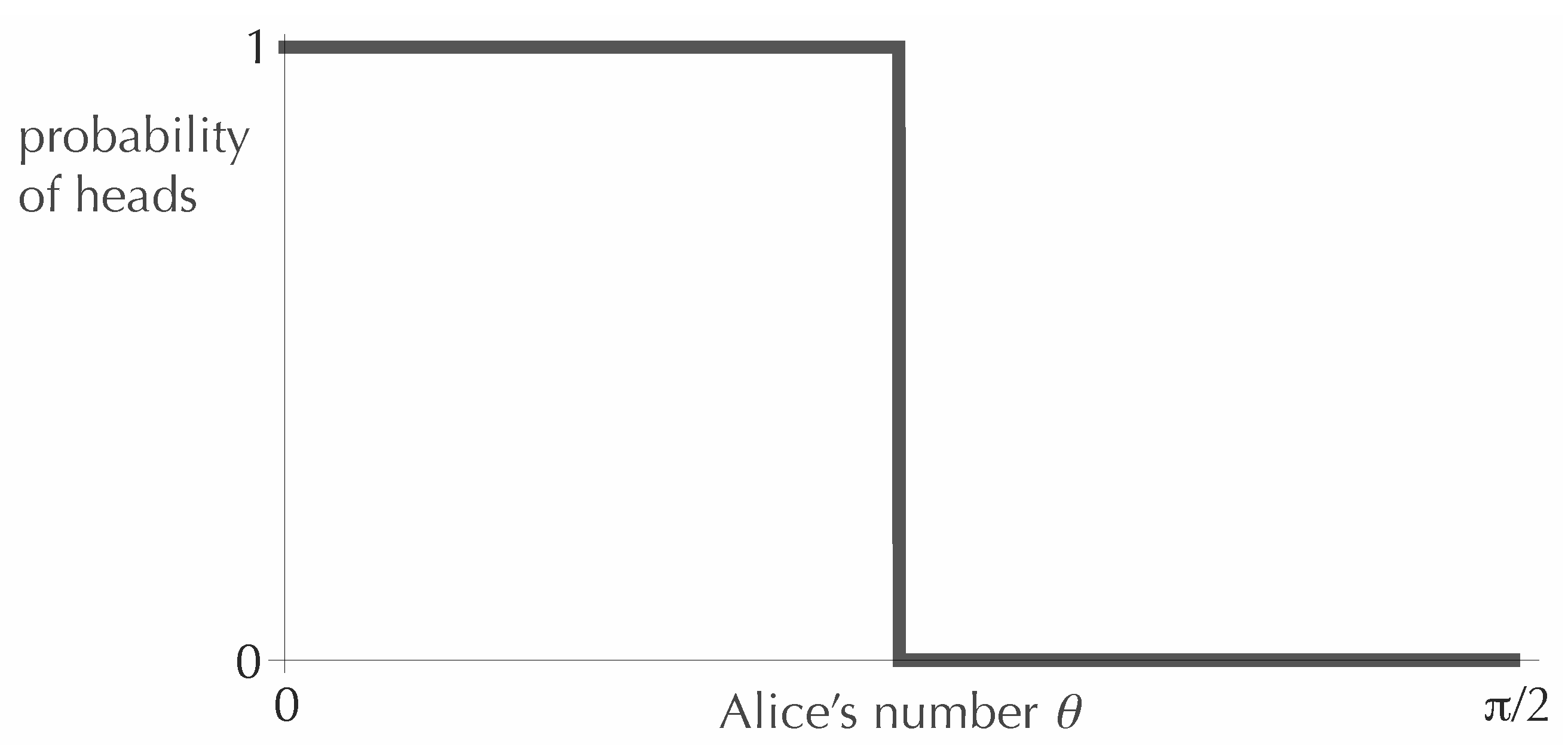Then, from his single toss, Bob gains exactly one bit of information about the value of θ (that is, 0.693 nats), which is the most one could hope for in a binary experiment. The optimal function defining this strategy is shown in Figure 1.

Figure 1. An optimal function for encoding the value of θ in the value of the probability of heads, when the coin will be tossed exactly once.

Figure 1. An optimal function for encoding the value of θ in the value of the probability of heads, when the coin will be tossed exactly once.

Note that one can obtain other optimal functions by cutting the graph in Figure 1 into any number of vertical strips and reordering the strips. All that matters is the weight (that is, the fraction of the interval $0\le \theta \le \pi /2$) assigned to each value of p. For larger values of N, there will similarly be many optimal graphs related to each other by a reordering of strips. In what follows, for definiteness, we will typically pick out the unique non-increasing optimal function.

As we increase the number of tosses, the optimal curve will continue to be a step function, with the number of steps tending to increase as N increases. We show below that the number of distinct probabilities represented in the optimal function $p\left(\theta \right)$ will not be larger than $\lfloor N/2\rfloor +2$, but this bound is likely to be rather weak as N gets large. One might guess that the number of steps instead grows as the square root of N, since the size of the statistical fluctuations in the frequency of occurrence of heads diminishes as $1/\sqrt{N}$. That is, it is plausible that one could distinguish approximately $\sqrt{N}$ distinct probability values reasonably well in N tosses. However, it is also quite conceivable that the problem is more subtle than this. Fortunately, for our purposes, we do not need to know precisely how the number of steps depends on N.

It is helpful, though, to re-express the mutual information in terms of a discrete set of probabilities $p_k$, with $k=1,\dots ,L$, rather than in terms of the function $p\left(\theta \right)$. Let $w_k$ be the weight assigned to the probability $p_k$. For the optimal function presented in Figure 1, for example, the values $p_k$ are zero and one, and the weight of each is 1/2, since each probability value occupies half of the interval $0\le \theta \le \pi /2$. In terms of $p_k$ and $w_k$, the mutual information is:

$$I(\theta :n)=-\sum _{n=0}^{N}P\left(n\right)lnP\left(n\right)+\sum _{k=1}^L{w}_k\sum _{n=0}^{N}P\left(n\right|p_k)lnP\left(n\right|p_k)$$

(8)

Here, again, $P\left(n\right|p_k)$ is the binomial distribution given in Equation (6)—the probability of getting exactly n heads in N tosses when the probability of heads in a single toss is $p_k$—and $P\left(n\right)={\sum }_k{w}_{k}P\left(n\right|p_k)$ is the overall probability of getting n heads. Our problem is to maximize $I(\theta :n)$ over all values of the parameters L, $p_k$ and $w_k$, where each $p_k$ and $w_k$ lies in the interval $[0,1]$ and the $w_k$s sum to unity.

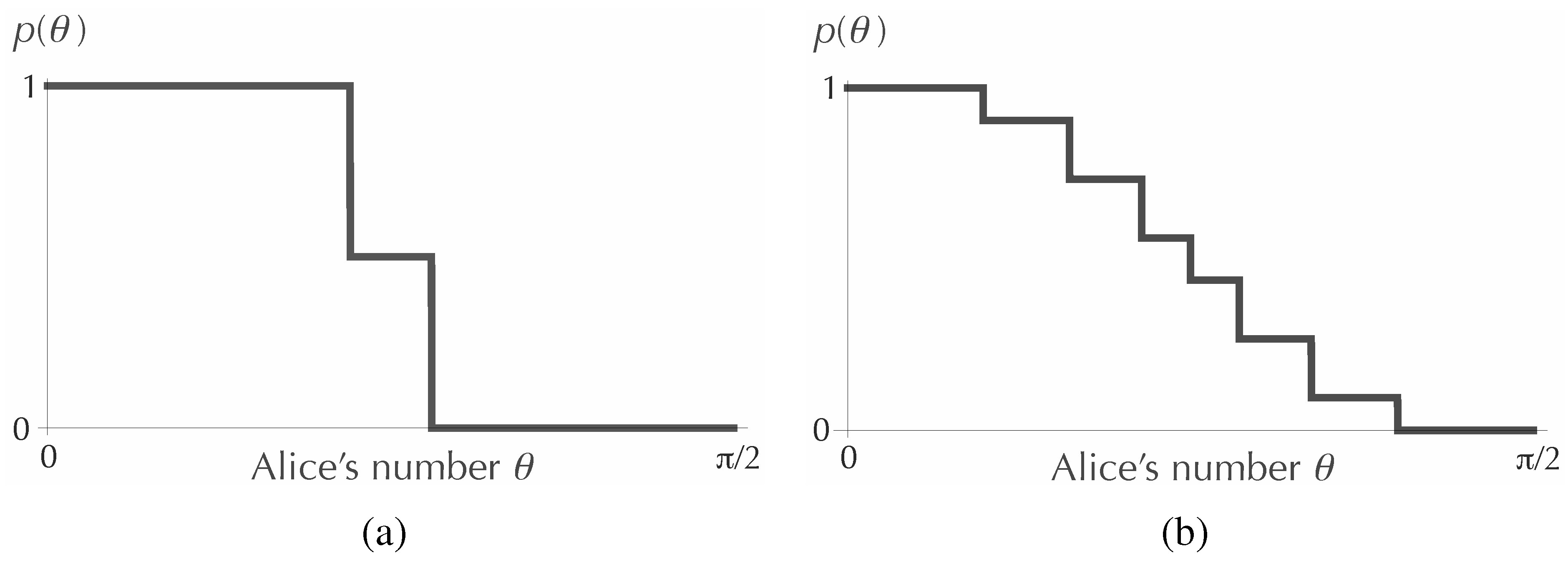
For two tosses of the coin (that is, for $N=2$), it is possible to solve the maximization problem analytically. One finds for this case that it is best for Alice to use exactly three probability values, namely, zero, 1/2 and one, with weights 15/34, 4/34 and 15/34, respectively. The first graph in Figure 2 shows the non-decreasing function $p\left(\theta \right)$ obtained from these values. For larger N, one can try to find the optimal values of the parameters numerically. The second graph in Figure 2 shows the function $p\left(\theta \right)$ resulting from a numerical optimization for $N=25$. Here, the number of distinct probability values, L, is also determined numerically. For example, starting from the $N=25$ graph in Figure 2, if we offer the computer program an additional probability value, it will simply set the new probability to be equal to one of the values already being used, so that the graph will not change. 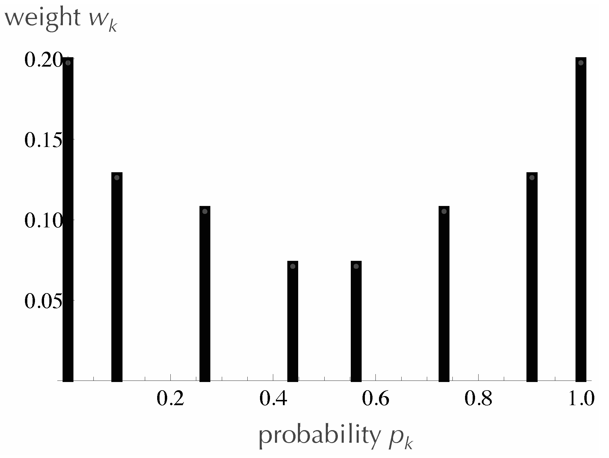Figure 3 shows explicitly the optimal choices for the $p_k$s for $N=25$, along with the weight, $w_k$, assigned to each.

Figure 2. Optimal functions for encoding the value of θ in the value of the probability of heads, when the coin will be tossed exactly twice (a) and 25 times (b). The corresponding maximum values of the mutual information are $I=0.754$ for $N=2$ and $I=1.570$ for $N=25$.

Figure 2. Optimal functions for encoding the value of θ in the value of the probability of heads, when the coin will be tossed exactly twice (a) and 25 times (b). The corresponding maximum values of the mutual information are $I=0.754$ for $N=2$ and $I=1.570$ for $N=25$.

Figure 3. A bar graph showing the specific probabilities that optimize $I(\theta :n)$ for the case of 25 tosses, along with the weight assigned to each probability.

Figure 3. A bar graph showing the specific probabilities that optimize $I(\theta :n)$ for the case of 25 tosses, along with the weight assigned to each probability.

2.2. An Upper Bound on the Number of Distinct Probability Values

We now show, as promised, that for any value of N, the number of distinct probability values used in an optimal strategy will not exceed $\lfloor N/2\rfloor +2$. For this purpose, it is helpful to write the mutual information in yet another form. Rather than characterizing Bob’s experimental result only by the number of heads, we can think of his result as a specific sequence, s, of heads and tails. Of course, any details of the sequence beyond the overall number of heads will not help Bob estimate θ, but including those details helps us with the mathematics. We have:

$$I(\theta :n)=I(\theta :s)=-\sum _{s}P\left(s\right)lnP\left(s\right)+\sum _{k=1}^L{w}_k\sum _{s}P\left(s\right|p_k)lnP\left(s\right|p_k)$$

(9)

where $P\left(s\right|p)$ is simply $p^n{(1-p)}^{N-n}$ for a sequence with n heads and $P\left(s\right)$ is the average ${\sum }_k{w}_{k}P\left(s\right|p_k)$. Because each toss is independent, the N-toss entropy, $-{\sum }_{s}P\left(s\right|p_k)lnP\left(s\right|p_k)$, is equal to N times the one-toss entropy, and we can write:

$$I(\theta :n)=-\sum _{s}P\left(s\right)lnP\left(s\right)-N\sum _{k=1}^L{w}_k{h}_2\left(p_k\right)$$

(10)

where $h_2$ is the binary entropy function, $h_2\left(x\right)=-[xlnx+(1-x)ln(1-x)]$. It is always optimal to include among the $p_k$s the special probabilities, zero and one, so let us fix the values $p_1=0$ and $p_L=1$. To look for the other $p_k$s, as well as for the $w_k$s, we introduce a Lagrange multiplier, λ, and define:

$$\tilde{I}=-\sum _{s}P\left(s\right)lnP\left(s\right)-N\sum _{k=1}^L{w}_k{h}_2\left(p_k\right)-\lambda \sum _{k=1}^L{w}_k$$

(11)

We now set $d\tilde{I}/d{w}_k$ equal to zero for each $k=1,\dots ,L$, and we set $d\tilde{I}/d{p}_k$ equal to zero for each $k=2,\dots ,L-1$. The former condition gives us:

$$0=-\frac{1}{N}\sum _s{p}_k^{n_s}{(1-p_k)}^{N-n_s}lnP\left(s\right)-\left(\frac{\lambda +1}{N}\right)-h_2\left(p_k\right)$$

(12)

where $n_s$ is the number of heads in the sequence s, while the latter condition yields:

$$0=-\sum _s\left[\left(\frac{n_s}{N}-p_k\right)p_k^{n_s-1}{(1-p_k)}^{N-n_s-1}lnP\left(s\right)\right]+ln{p}_k-ln(1-p_k)$$

(13)

Suppose now that we have found a solution, $\left\{(p_k,w_k)\right\}$, to Equation (12) and Equation (13). From $\left\{(p_k,w_k)\right\}$, we compute the numbers $P\left(s\right)$. With the values of $P\left(s\right)$ fixed, consider the function:

$$r\left(x\right)=-\frac{1}{N}\sum _s{x}^{n_s}{(1-x)}^{N-n_s}lnP\left(s\right)-\left(\frac{\lambda +1}{N}\right)-h_2\left(x\right)$$

(14)

which is defined on the interval $0\le x\le 1$. (The values $r\left(0\right)$ and $r\left(1\right)$ are defined by taking the limits $x\to 0$ and $x\to 1$.) Notice that Equation (12) and Equation (13) imply the following facts about the $p_k$s:

$$r\left(p_k\right)=0,\text{for}k=1,\dots ,L,\text{and}{r}^{\prime }\left(p_k\right)=0,\text{for}k=2,\dots ,L-1$$

(15)

Thus, it must be the case that each $p_k$, including $p_1=0$ and $p_L=1$, is a root of the function $r\left(x\right)$, and except at the two endpoints, these roots must occur where the function has zero slope. Therefore, we can get a bound on the number of distinct probability values by finding a bound on the number of values of x in the interval $(0,1)$ for which $r\left(x\right)$ is tangent to the x-axis. (If the maximum of I occurs at the boundary of the allowed region of the $w_k$s, that is, at the boundary of the probability simplex, then the maximum need not satisfy Equation (12) and Equation (13). What this means, though, is that we have set L to be larger than it needs to be. We can reduce the size of L, until the maximum occurs in the interior of the simplex. Similarly, if a maximum occurs when one of the probabilities $p_2,\dots ,p_{L-1}$ is zero or one, we can achieve the same maximum with a smaller value of L and with the extreme values taken only by $p_1$ and $p_L$.)

Note that $r\left(x\right)$ is of the form $r\left(x\right)=t\left(x\right)-h_2\left(x\right)$, where $t\left(x\right)$ is a polynomial of degree N. We can write the second derivative of $r\left(x\right)$ as:

$$r^{\prime \prime }\left(x\right)=\frac{t^{\prime \prime }\left(x\right)x(1-x)+1}{x(1-x)}$$

(16)

in which the numerator is also a polynomial of degree N. Therefore, $r^{\prime \prime }\left(x\right)$ can be zero for at most N distinct values of x in the interval $(0,1)$. Since $r\left(x\right)$ is equal to zero at both endpoints, each point $x_k$ in the interval $(0,1)$ for which $r\left(x_k\right)=0$ and $r^{\prime }\left(x_k\right)=0$ must be flanked by two points, $x_k^{(-)}$ and $x_k^{(+)}$, at which the second derivative is zero, and the pairs $\{x_k^{(-)},x_k^{(+)}\}$ and $\{x_j^{(-)},x_j^{(+)}\}$ will not have a point in common if $j\ne k$. Thus, the number of such points $x_k$ can be at most $\lfloor N/2\rfloor$. When we add in the roots $x=0$ and $x=1$, we find that the total number L of distinct probability values must satisfy $L\le \lfloor N/2\rfloor +2$, which is what we wanted to show.

Looking again at Figure 1 and Figure 2, we see that this bound is saturated for $N=1$ and $N=2$, for which $L=2$ and $L=3$, respectively. However, for $N=25$, we have $L=8$, which is significantly less than $\lfloor N/2\rfloor +2=14$.

2.3. Letting the Number of Trials Go to Infinity

We now want to consider the limit of a large number of tosses. To do this, we find that it is more convenient to return to the form of $I(\theta :n)$ given in Equation (8), in which the result of Bob’s experiment is characterized simply by the number of heads. Starting from that expression, introducing the Lagrange multiplier, λ, as before, and setting $d\tilde{I}/d{w}_k$ equal to zero, we get the condition:

$$-\sum _{n=0}^{N}P\left(n\right|p_k)lnP\left(n\right)=\lambda +1-\sum _{n=0}^{N}P\left(n\right|p_k)lnP\left(n\right|p_k)$$

(17)

(We do not need the condition $d\tilde{I}/d{p}_k=0$ for the asymptotic calculation.) As the number of trials increases, Bob will be able to discriminate among values of $p_k$ that are more and more closely spaced. We therefore expect the optimal discrete distributions analogous to the one shown in Figure 3 to approach (in measure) a continuous distribution, $w\left(p\right)$, where $w\left(p\right)dp$ is the weight assigned to an infinitesimal interval of width $dp$ around the value p. We now aim to find this continuous distribution. We proceed by means of a simple heuristic argument. It will turn out that the function $w\left(p\right)$ that we find by this method agrees with what has been obtained more rigorously in [14] and [15]. (I confess, though, that there is still a mathematical gap—the work in [14] and [15] considers from the outset only continuous distributions, whereas we are now thinking of an infinite sequence of discrete distributions.)

First, as N increases, the binomial distribution, $P\left(n\right|p_k)$, given in Equation (6), becomes highly peaked around the value $N{p}_k$. That is, the value of n will be largely determined by the value $p_k$. When we average $P\left(n\right|p_k)$ over all the values of k, we should, therefore, find that the distribution $P\left(n\right)$ is very close to $(1/N)w(n/N)$. That is, the a priori distribution of n should closely mirror the distribution of probability values that Alice will use. (The factor $1/N$ accounts for the fact that $P\left(n\right)$ is normalized by a sum over the values $n=0,\dots ,N$, whereas $w\left(p\right)$ is normalized by an integral over the interval $0\le p\le 1$.) Let us assume that for the purpose of finding the limiting distribution, we may take $P\left(n\right)$ to be equal to $(1/N)w(n/N)$. Consider, then, the left-hand side of Equation (17), which we now write as:

$$-\sum _{n=0}^{N}P\left(n\right|p_k)ln\left[\frac{w(n/N)}{N}\right]$$

(18)

Again, when N is large, the function $P\left(n\right|p_k)$ is sharply peaked around the value $n=N{p}_k$, so in the factor $ln\left[w\right(n/N)/N]$, we replace $n/N$ with $p_k$. Thus, Equation (17) can be approximated as:

$$-ln\left[\frac{w\left(p_k\right)}{N}\right]=\lambda +1-\sum _{n=0}^{N}P\left(n\right|p_k)lnP\left(n\right|p_k)$$

(19)

The sum on the right-hand side (including the negative sign) is the entropy of the binomial distribution for N trials with probabilities $p_k$ and $(1-p_k)$. For large N, this entropy can be approximated as [16]:

$$-\sum _{n=0}^{N}P\left(n\right|p_k)lnP\left(n\right|p_k)\approx \frac{1}{2}\left(lnN+1+ln\left[2\pi p_k(1-p_k)\right]\right)$$

(20)

with an error that diminishes as $1/N$. Making this substitution in Equation (19), we get that for each value of k:

$$w\left(p_k\right)=\frac{C}{\sqrt{p_k(1-p_k)}},$$

(21)

where C is independent of k. (Note that $w\left(p_k\right)$ is very different from $w_k$, in that $w\left(p\right)$ takes into account not just the weights of the values $p_k$, but also their spacing, which may vary over the interval $[0,1]$.) Since the values $p_k$ will become very closely spaced, we conclude that the optimal weighting function, in the limit $N\to \infty$, is of the form $w\left(p\right)=C/\sqrt{p(1-p)}$. The constant, C, is determined by the requirement that the integral of $w\left(p\right)$ over the interval $0\le p\le 1$ is unity, and we arrive at:

$$w\left(p\right)=\frac{1}{\pi \sqrt{p(1-p)}}$$

(22)

We now work out the unique non-increasing function, $p\left(\theta \right)$, corresponding to the weighting function, $w\left(p\right)$, of Equation (22). First, we find the inverse of $p\left(\theta \right)$, which we call $\theta \left(p\right)$. 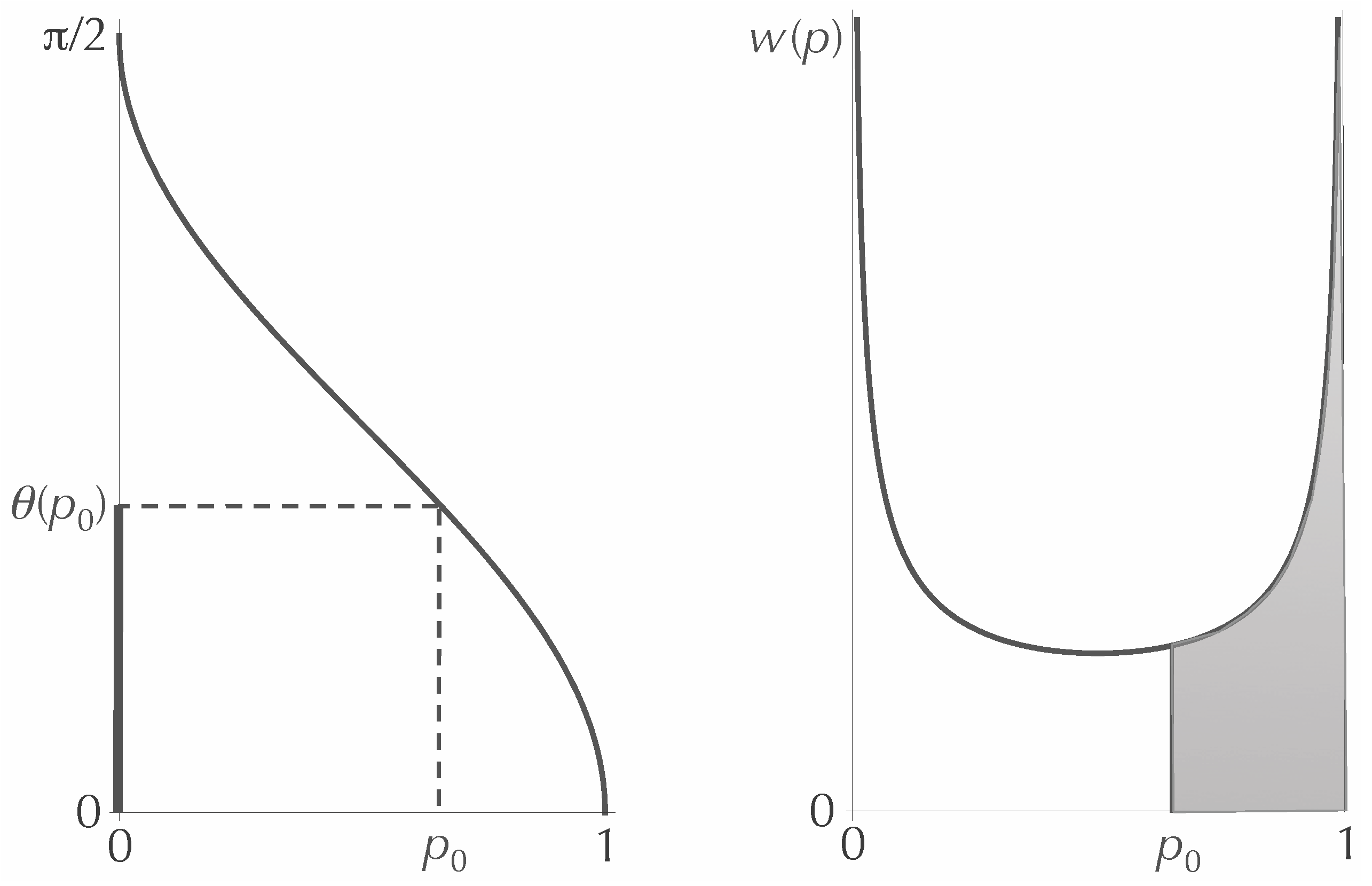For any $p_0$ between zero and one, the weight assigned to the interval $[p_0,1]$ is the same as the fraction of the interval $[0,\pi /2]$ that lies between zero and $\theta \left(p_0\right)$ (see Figure 4). That is:

$$\theta \left(p_0\right)=\frac{\pi }{2}{\int }_{p_0}^{1}w\left(p\right)dp=\frac{1}{2}{\int }_{p_0}^1\frac{1}{\sqrt{p(1-p)}}dp$$

(23)

The integral can be evaluated by making the substitution $p={sin}^2\varphi$, and one finds that:

$$\theta \left(p_0\right)=\frac{\pi }{2}-{sin}^{-1}\sqrt{p_0}$$

(24)

Inverting the function, we get:

$$p\left(\theta \right)={cos}^2\theta$$

(25)

That is, if Alice must convey the value of θ by sending Bob a coin with probability $p\left(\theta \right)$ of heads, in the limit of a large number of tosses, she can convey the most information by choosing the encoding function $p\left(\theta \right)={cos}^2\theta$.

Figure 4. The functions $\theta \left(p\right)$ and $w\left(p\right)$. The ratio of $\theta \left(p_0\right)$ to $\pi /2$ should be equal to the shaded area under the curve $w\left(p\right)$.

Figure 4. The functions $\theta \left(p\right)$ and $w\left(p\right)$. The ratio of $\theta \left(p_0\right)$ to $\pi /2$ should be equal to the shaded area under the curve $w\left(p\right)$.

What is intriguing about this result is that the function ${cos}^2\theta$ is the one nature uses to “encode” the polarization angle, θ, of a linearly polarized photon in the probability of the vertical outcome in a horizontal vs. vertical measurement. Thus, in this particular physical situation, nature is using an optimal encoding. Note how very different the above derivation is from the usual derivation of the curve $p\left(\theta \right)={cos}^2\theta$ in quantum mechanics. Normally, we obtain this function by squaring the magnitude of the component of the state vector corresponding to the outcome “vertical.” However, in the above argument, there is no state vector.

One might worry that in nature, the angle of polarization is not limited to the range $0\le \theta \le \pi /2$. In order to accommodate all the linear polarizations, we need to let θ go up to π, in which case ${cos}^2\theta$ is not a decreasing function. However, this fact does not affect the optimality of the cosine squared curve. The function $p\left(\theta \right)={cos}^2\theta$ maximizes the mutual information (in the limit of infinite N), even when θ ranges over the interval $0\le \theta \le \pi$. It is true that with this larger interval, a given value of n will typically lead to a probability distribution over θ that has two peaks, corresponding to the two distinct values of θ for which ${cos}^2\theta$ is equal to $n/N$. However, the amount of information Bob gains about θ in this case is the same as the amount he gains when his final distribution has only one peak, but extends over only half of the interval. A rough analogy is this: the amount of information one gains by learning that the value shown on a standard six-sided die is either a one or a six is the same as the amount of information one gains by learning that the value shown on a three-sided die is a one. Extending this observation, we can identify other probability functions that achieve, in the large N limit, the same optimal value of the mutual information as the function ${cos}^2\theta$, namely, functions of the form ${cos}^2(m\theta /2)$, where m is a positive integer and θ ranges from zero to $2\pi$. The curve with $m=1$, that is, $p\left(\theta \right)={cos}^2(\theta /2)$, can be recognized as the probability of getting the outcome “vertical” in a spin measurement of a spin-1/2 particle, if the initial direction of spin makes an angle θ with the vertical.

The agreement between the solution to our communication problem and the probability law that appears in quantum theory for the case of linear polarization of photons (or for a measurement of spin for a spin-1/2 particle) might suggest the possibility of deriving at least part of the structure of quantum theory from a “principle of optimal information transfer.” Indeed, as we will see in the next section, the above result generalizes, in a straightforward way, to measurements with more than two possible outcomes. However, as I explain in the following paragraph, the project of finding such a derivation appears to be thwarted, or at least impeded, by the fact that in quantum theory, probability amplitudes are complex rather than real.

The above solution to our communication problem is optimal only under the assumption that the a priori distribution of the variable θ is the uniform distribution. Indeed, if we imagine an observer trying to ascertain the angle of polarization of a beam of linearly polarized light, it is plausible to assume a uniform prior distribution over all angles of polarization. This is the unique distribution that is invariant under rotations and reflections, which are the only unitary transformations that take linear polarizations into linear polarizations. Therefore, one can say that our assumption of a uniform distribution over θ agrees with what is natural in the case of linear polarization. However, with regard to the basic structure of quantum theory, the linear polarizations do not play any special role. They can be represented by state vectors with real components, but to get the full set of pure states, we should use complex state vectors. It is thus much more natural to assume a uniform distribution over the entire sphere of possible polarizations (including elliptical and circular polarizations) on which the linear polarizations form a great circle. (The same issue arises in the case of a spin-1/2 particle, for which the set of pure states again forms a sphere.) The uniform distribution over the sphere is the unique distribution that is invariant under all rotations of the sphere, which correspond to the full set of unitary transformations of the quantum state. Let γ be the angle on the sphere measured from the “north pole.” Then, the uniform distribution over the sphere entails a uniform distribution of the variable $cos\gamma$ over the range $-1\le cos\gamma \le 1$; or, to make the problem more similar to the case considered above, we can say that the variable $\eta =(\pi /4)(1-cos\gamma )$ is distributed uniformly over the interval $0\le \eta \le \pi /2$. Now, according to our solution to the communication problem, the state will be expressed optimally in the probabilities of the two outcomes of an orthogonal measurement (in the limit of a large number of trials) if the probability of one of those outcomes is given by ${cos}^2\eta$, which, as a function of γ, would be $p\left(\gamma \right)={cos}^2\left[(\pi /4)(1-cos\gamma )\right]$. This is not what nature actually does. If we take the two outcomes of the measurement to correspond to the north and south poles of the sphere, then the probability of the first outcome is, in real life, given by $p\left(\gamma \right)={cos}^2(\gamma /2)$, which is not the same as $p\left(\gamma \right)={cos}^2\left[(\pi /4)(1-cos\gamma )\right]$ and is not optimal (because γ is not uniformly distributed).

In Section 4, we ask whether an alternative version of the problem might be more friendly toward complex amplitudes, but first, we show how the Alice-Bob communication problem generalizes to a measurement with more than two outcomes.

3. Encoding Several Parameters in an Equal Number of Independent Probabilities

We now consider a natural generalization of the problem of Section 2. Instead of a coin, Alice sends Bob a d-sided die, and instead of trying to convey a single real variable, θ, she is trying to convey the value of a variable, $\overrightarrow{a}$, that varies over a $(d-1)$-dimensional manifold. Once he receives the die, Bob will roll it N times in order to gain information about the probabilities of the d possible outcomes and, thereby, to gain information about $\overrightarrow{a}$. As in Section 2, we assume that the optimal strategy in the limit of a large number of trials can be expressed by specifying a weighting function over probability space. This weighting function will be our main focus for now. At the end of this section, we show how the optimal weighting function corresponds to a particular distribution of a variable $\overrightarrow{a}$.

In the present case, probability space has $d-1$ dimensions, since the d probabilities of the outcomes of the experiment (a roll of the die) must sum to unity. Let us use the symbol $\overrightarrow{p}$ to indicate a point in this probability space—$\overrightarrow{p}=(p_1,p_2,\dots ,p_d)$—where $p_{\alpha }$ is the probability of outcome α. Each value of $\overrightarrow{p}$ represents a particular kind of die that Alice could send to Bob, with specific probabilities of the d outcomes of a roll. Bob now rolls the die. Let $n_{\alpha }$ be the number of times Bob gets the outcome α when he rolls the die N times, and let $\overrightarrow{n}$ be the ordered set of values $\overrightarrow{n}=(n_1,\dots ,n_d)$. Thus, $\overrightarrow{p}$ represents the die Alice sends, and $\overrightarrow{n}$ represents the result of Bob’s N trials.

For any finite value of N, we expect the optimal strategy to consist of (i) choosing a finite set of points, ${\overrightarrow{p}}_k$, of probability space to be used and (ii) for each $p_k$, choosing the probability, $w_k$, with which ${\overrightarrow{p}}_k$ will be used. Here, ${\sum }_k{w}_k=1$. The quantity to be maximized is again the mutual information, which can be written in a form parallel to that of Equation (8):

$$I=-\sum _{\overrightarrow{n}}P\left(\overrightarrow{n}\right)lnP\left(\overrightarrow{n}\right)+\sum _{k=1}^L{w}_k\sum _{\overrightarrow{n}}P\left(\overrightarrow{n}\right|{\overrightarrow{p}}_k)lnP\left(\overrightarrow{n}\right|{\overrightarrow{p}}_k)$$

(26)

where $P\left(\overrightarrow{n}\right)$ can be written as ${\sum }_{k=1}^L{w}_{k}P\left(\overrightarrow{n}\right|{\overrightarrow{p}}_k)$. In this expression, each sum over $\overrightarrow{n}$ is over all sets of non-negative integers $(n_1,\dots ,n_d)$ such that $n_1+n_2+\cdots +n_d=N$, and $P\left(\overrightarrow{n}\right|{\overrightarrow{p}}_k)$ is the multinomial distribution:

$$P\left(\overrightarrow{n}\right|\overrightarrow{p})=\frac{N!}{n_1!n_2!\cdots n_d!}{p}_1^{n_1}{p}_2^{n_2}\cdots p_d^{n_d}$$

(27)

As an example, consider the case $d=3$ and $N=2$; that is, Alice sends Bob a three-sided die and Bob rolls it only twice. For this case, a combination of analytic and numerical calculations indicates that the mutual information is maximized by using exactly six different points in probability space, namely:

$$\begin{array}{c}\hfill {\overrightarrow{p}}_1=(1,0,0){\overrightarrow{p}}_2=(0,1,0){\overrightarrow{p}}_3=(0,0,1)\\ \hfill {\overrightarrow{p}}_4=(1/2,1/2,0){\overrightarrow{p}}_5=(1/2,0,1/2){\overrightarrow{p}}_6=(0,1/2,1/2)\end{array}$$

(28)

That is, there are six different kinds of die that Alice could send. The optimal probabilities with which she sends each kind of die come out to be $w_1=w_2=w_3=7/27$ and $w_4=w_5=w_6=2/27$. The amount of information Alice is able to convey to Bob by this method is $I=3ln(3/2)=1.216$ nats.

As N gets very large, we expect that the discrete set of points ${\overrightarrow{p}}_k$ in probability space, together with their weights, $w_k$, will again approach a continuous distribution, $w\left(\overrightarrow{p}\right)$. Let us interpret the function $w\left(\overrightarrow{p}\right)$ as a distribution relative to the normalized Euclidean measure over the probability simplex, so that the normalization condition for $w\left(\overrightarrow{p}\right)$ is:

$$(d-1)!{\int }_0^{\infty }\cdots {\int }_0^{\infty }w\left(\overrightarrow{p}\right)\delta (p_1+\cdots +p_d-1)d{p}_1\cdots d{p}_d=1$$

(29)

Here, δ is the Dirac delta function. (For example, the constant function, $w\left(\overrightarrow{p}\right)=1$, counts as a properly normalized distribution.)

The argument leading to the optimal function in the limit of large N proceeds very much as in Section 2. The analog of Equation (19) is:

$$-ln\left[\frac{(d-1)!w\left(\overrightarrow{p}\right)}{N^{d-1}}\right]=\lambda +1-\sum _{\overrightarrow{n}}P\left(\overrightarrow{n}\right|\overrightarrow{p})lnP\left(\overrightarrow{n}\right|\overrightarrow{p})$$

(30)

The sum on the right-hand side (together with the negative sign) is now the entropy of a multinomial distribution, which, up to an error of order $1/N$, can be approximated as [16]:

$$-\sum _{\overrightarrow{n}}P\left(\overrightarrow{n}\right|\overrightarrow{p})lnP\left(\overrightarrow{n}\right|\overrightarrow{p})\approx \left(\frac{d-1}{2}\right)\left[lnN+1+ln\left(2\pi \right)\right]+\frac{1}{2}ln(p_1{p}_2\cdots p_d)$$

(31)

Inserting this approximation into Equation (30), we arrive at the form:

$$w\left(\overrightarrow{p}\right)=\frac{C}{\sqrt{p_1{p}_2\cdots p_d}}$$

(32)

of which Equation (21) is a special case. Again, this result is consistent with the results of [14] and [15].

Though it is not crucial for our purposes to find the value of C, it is worth doing the calculation, because it will help us interpret the function $w\left(\overrightarrow{p}\right)$. We require:

$$(d-1)!{\int }_0^{\infty }\cdots {\int }_0^{\infty }\frac{C}{\sqrt{p_1{p}_2\cdots p_d}}\delta (p_1+\cdots +p_d-1)d{p}_1\cdots d{p}_d=1$$

(33)

The integral can be evaluated by changing the integration variables to $a_1,\dots ,a_d$, where $p_{\alpha }=a_{\alpha }^2$. That is, we write each probability as the square of a real amplitude. Then $d{p}_{\alpha }$ is equal to $2a_{\alpha }d{a}_{\alpha }$, and the factor $a_{\alpha }$ cancels the factor $\sqrt{p_{\alpha }}$ in the denominator. For simplicity, we extend the range of integration, so that it encompasses the entire sphere defined by $a_1^2+\cdots +a_d^2=1$ (not just the positive section of the sphere), and we compensate by dividing by $2^d$. Equation (33) then becomes:

$$(d-1)!C{\int }_{-\infty }^{\infty }\cdots {\int }_{-\infty }^{\infty }\delta (a_1^2+\cdots +a_d^2-1)d{a}_1\cdots d{a}_d=1$$

(34)

In terms of the radial coordinate, $r=\sqrt{a_1^2+\cdots +a_d^2}$, we can write this condition as:

$$(d-1)!C{S}_{d-1}{\int }_0^{\infty }\delta (r^2-1)dr=1$$

(35)

where $S_{d-1}$ is the “surface area” of the $(d-1)$-dimensional unit sphere in d dimensions. Replacing $\delta (r^2-1)$ with $(1/2)\delta (r-1)$, we find that:

$$C=\frac{2}{(d-1)!S_{d-1}}$$

(36)

Finally, from the formula, $S_{d-1}=2{\pi }^{d/2}/\Gamma (d/2)$, we get:

$$C=\frac{\Gamma (d/2)}{{\pi }^{d/2}(d-1)!}$$

(37)

In addition to giving us the value of C, the above calculation shows that the optimal distribution, $w\left(\overrightarrow{p}\right)$, over the probability simplex corresponds to the uniform distribution over the sphere of unit vectors, $\overrightarrow{a}$, when we write $p_{\alpha }=a_{\alpha }^2$. Thus, we have the following result: if Alice wants to convey to Bob the value of a uniformly distributed unit vector, $\overrightarrow{a}$, in ${\mathbb{R}}^d$, by encoding the vector in the probabilities of the outcomes of a d-sided die, and if Bob will be allowed to roll the die a large number of times, then Alice and Bob will optimize the information transfer (in the limiting case) by choosing the encoding function $p_{\alpha }=a_{\alpha }^2$. One might be concerned about the fact that the probabilities will not tell Bob the signs of the components $a_{\alpha }$, but this fact does not affect the value of the mutual information. A distribution with $2^d$ narrow peaks over the entire unit sphere in d dimensions provides as much information about a uniformly distributed unit vector as a single-peaked distribution provides about a unit vector that was already confined to the positive section of the sphere. (We encountered a similar issue in Section 2, when we extended the range of θ beyond the interval $0\le \theta \le \pi /2$.)

In the real-vector-space variant of quantum theory, a pure state is represented by a real unit vector, and the probabilities of the outcomes of a complete orthogonal measurement are given by the squared components of the state vector in the basis representing the measurement. Thus, according to what we have just found, real-vector-space quantum theory exhibits the property of optimal information transfer from the preparation of a pure state to the outcome of a measurement, in the limit of a large number of trials of the experiment. However, this conclusion does not carry over to the case of actual quantum theory. In the real-vector-space theory, the uniform distribution over the unit sphere in state space corresponds to the distribution $w\left(\overrightarrow{p}\right)=C/\sqrt{p_1{p}_2\cdots p_d}$ over the probability simplex. In contrast, in standard quantum theory, with a complex state space, it was shown by Sýkora that the uniform distribution over the unit sphere corresponds to the uniform distribution over the probability simplex in the sense of the Euclidean measure [17]. That is, in standard quantum theory, we would have $w\left(\overrightarrow{p}\right)=1$, which is not the optimal distribution for conveying information. We now ask whether by thinking differently about the problem of optimal information transfer, we might get a result that is consistent with complex probability amplitudes.

4. Can We Get Complex Amplitudes?

We present here two distinct approaches toward reconciling the above results with the fact that quantum probability amplitudes are complex. First, we try changing the way we apply our result to quantum theory; then, we consider changing the optimization problem itself.

4.1. Information about a Unitary Transformation

It is conceivable that standard quantum theory does exhibit, in some way, the property of optimal information transfer, but that we have not been imagining the right physical correlate of our Alice-Bob communication problem. We have been imagining the preparation of a pure state followed directly by a measurement. As an alternative, consider the following scenario: A pair of qubits are prepared in the maximally entangled state $|{\Phi }^{+}\rangle =(1/\sqrt{2})\left(\right|00\rangle +|11\rangle )$, where $|0\rangle$ and $|1\rangle$ are orthogonal states of a single qubit. The two qubits are then sent to two experimenters, Alice and Bob. Alice performs on her qubit a unitary transformation, U (which we will represent as a unit-determinant unitary matrix), and then sends her qubit to Bob. Now that he is in possession of both qubits, Bob performs the Bell measurement, that is, the measurement whose outcomes correspond to the four orthogonal states:

$$\begin{array}{c}\hfill |{\Phi }^{+}\rangle =(1/\sqrt{2})\left(\right|00\rangle +|11\rangle )|{\Phi }^{-}\rangle =(1/\sqrt{2})\left(\right|00\rangle -|11\rangle )\\ \hfill |{\Psi }^{+}\rangle =(1/\sqrt{2})\left(\right|01\rangle +|10\rangle )|{\Psi }^{-}\rangle =(1/\sqrt{2})\left(\right|01\rangle -|10\rangle )\end{array}$$

(38)

(see Figure 5). We imagine that the same experiment, with the same transformation, U, is repeated many times, and from the frequencies of occurrence of the four outcomes, Bob tries to gain information about U. We can ask whether the quantum mechanical rule that relates U to the probabilities of Bob’s outcomes conveys information about U optimally, in the limit of a large number of trials.

Figure 5. Alice performs a unitary transformation, U, on one of two qubits and sends it to Bob, who then performs the four-outcome Bell measurement on the pair.

Figure 5. Alice performs a unitary transformation, U, on one of two qubits and sends it to Bob, who then performs the four-outcome Bell measurement on the pair.

It happens that the answer to this question is: yes! The group of special unitary transformations in two dimensions can be pictured as the three-dimensional surface of a unit sphere in four dimensions, and the natural a priori measure on this sphere is the uniform measure: this is the unique measure invariant under the action of the group. Moreover, the probabilities of the outcomes of Bob’s measurement can be represented as the squares of the components of a unit vector that defines a point on this sphere [15]. Thus, this physical situation exactly mirrors the optimal communication strategy we arrived at in the preceding section.

Unfortunately, there is no obvious way to generalize this result to higher-dimensional quantum systems. The most natural generalization to three dimensions, for example, would be this: Two qutrits are initially prepared in the maximally entangled state $(1/\sqrt{3})\left(\right|00\rangle +|11\rangle +|22\rangle )$. Alice applies to one of the qutrits a three-dimensional special unitary transformation, U, and then, Bob performs on the pair a generalized Bell measurement having nine possible outcomes. It turns out that in this case, the information about U is not conveyed optimally in the probabilities of the outcomes. The easiest way to see that the encoding is not optimal is to note that as Alice’s unitary transformation varies over the whole set of possible transformations, Bob’s probabilities do not vary over the whole probability simplex [15]. That is, a section of the probability space is not being used, and the communication is therefore not optimal. If Alice and Bob were free to make up their own probability rule rather than having to use the one provided by nature, Alice could convey more information to Bob.

It is conceivable that a different generalization of the above two-qubit scenario would exhibit optimal information transfer, but at present, I am not aware of such a generalization.

4.2. Two Messages in One Coin

A curious fact about standard quantum theory is this: the number of real parameters required to specify a pure state is exactly twice the number of independent probabilities characteristic of a complete orthogonal measurement. If the dimension of the state space is d, then there are $(d-1)$ independent probabilities of a d outcome measurement, but it takes $2(d-1)$ real numbers to specify a pure state. (The state vector has d complex components, each with a real and imaginary part; but normalization removes one degree of freedom, and the unobservable overall phase of the vector is normally not considered part of the specification of the state. The number of parameters remaining is, thus, $2d-2$.) In contrast, in our communication problem, we have assumed that the number of parameters being conveyed by Alice is exactly the same as the number of independent probabilities. In this sense, there is a mismatch between our communication problem and quantum theory, so it is perhaps not surprising that the optimal communication strategy does not show any hint of the complex-vector-space structure.

There are many ways in which one might imagine modifying our communication problem so as to capture the factor of two identified in the preceding paragraph. Here, I describe one such possibility, but I do not attempt in this paper to find the solution to this particular communication problem.

In our original problem, a single message was being conveyed to a single recipient. Let us now imagine that Alice has two “messages,” namely, two independently distributed real numbers, ${\theta }_1$ and ${\theta }_2$, to be conveyed, respectively, to two recipients, Bob and Charlie. As before, Alice must encode these numbers in the probability of heads of a coin, but we assume that a single coin will have to be used for both messages: the coin will be tossed N times, and both Bob and Charlie will see the results of these tosses, each trying to learn from these results something about the value of the variable, ${\theta }_1$ or ${\theta }_2$, that he is interested in. Let $p({\theta }_1,{\theta }_2)$ be the probability of heads. We ask what function or functions, $p({\theta }_1,{\theta }_2)$, maximize $min\{I({\theta }_1:n),I({\theta }_2:n)\}$. That is, we want to maximize the amount of information gained by the recipient who gains the least information. (This formulation of the problem tends to favor a symmetric solution.) We can write $I({\theta }_1:n)$, for example, as:

$$I({\theta }_1:n)=-\sum _{n=0}^{N}P\left(n\right)lnP\left(n\right)+〈\sum _{n=0}^{N}P\left(n\right|{\theta }_1)lnP\left(n\right|{\theta }_1)〉$$

(39)

where $P\left(n\right|{\theta }_1)=\int P\left(n\right|p({\theta }_1,{\theta }_2))d{\theta }_2$ and $P\left(n\right|p({\theta }_1,{\theta }_2))$ is the binomial distribution computed from the probability $p({\theta }_1,{\theta }_2)$, as in Equation (6). The angular brackets indicate an average over ${\theta }_1$.

Note that even in the case $N=1$, it is possible for Alice to convey a nonzero amount of information to both recipients. Suppose that ${\theta }_1$ and ${\theta }_2$ are both uniformly (and independently) distributed over the interval $[0,1]$. With $N=1$, Alice cannot do better than to use a deterministic strategy, and a natural choice for the function $p({\theta }_1,{\theta }_2)$ is:

$$p({\theta }_1,{\theta }_2)=\left\{\begin{array}{c}1\text{if}{\theta }_1<r\text{and}{\theta }_2<r\hfill \\ 0\text{otherwise}\hfill \end{array}\right.$$

(40)

where $r\in [0,1]$ is chosen to maximize the mutual information. With this form of the function $p({\theta }_1,{\theta }_2)$, both $I({\theta }_1:n)$ and $I({\theta }_2:n)$ come out to be:

$$I=h_2\left(r^2\right)-r{h}_2\left(r\right)$$

(41)

where, again, $h_2$ is the binary entropy function, $h_2\left(x\right)=-\left[xlnx+(1-x)ln(1-x)\right]$. The optimal value of r works out to be $r=0.714$, which makes both values of mutual information equal to 0.266. This is notably less than what Alice can convey to a single observer in one toss (that amount would be 0.693, as we have seen), but such a reduction is not surprising, given the compromise entailed in having to use the same coin for two independent messages.

The more interesting case would be to let N approach infinity, as we have done before. In this case, it is conceivable that one achieves the optimal information transfer only by using a highly discontinuous function $p({\theta }_1,{\theta }_2)$, for example, a function obtained by first using a space-filling curve to map the interval $0\le p\le 1$ into the square swept out by ${\theta }_1$ and ${\theta }_2$. Thus, it may also be interesting, as a separate problem, to limit $p({\theta }_1,{\theta }_2)$ to the set of continuous functions and to maximize the limiting value of $min\{I({\theta }_1:n),I({\theta }_2:n)\}$ under this restriction. Evidently, we can extend the problem to the case of d outcomes by replacing the coin with a die (but still, with only two recipients).

I would estimate as rather slim the chances that this particular version of the problem will happen to yield a result consistent with the rule for computing probabilities in standard quantum theory. Moreover, this extension of the problem is a bit artificial, in that the factor of two was put in by hand by positing two recipients. Still, it seems worthwhile to explore in future work this and other variations on our communication problem, to see whether there is some sense, short of restricting attention to real state vectors, in which nature optimizes the transfer of information.

5. Conclusion

To summarize, we have formulated a communication problem in which information is conveyed only through probabilities, and the receiver is allowed only a finite number of trials of his experiment. We have found the solution to this problem for a few special cases with a small number of trials, and we have used a simple heuristic argument to identify an optimal strategy when the number of trials approaches infinity. This limiting strategy is consistent with what we would see in nature if nature were described by the real-vector-space variant of quantum theory. We leave as an open question whether some modified version of our problem would lead to a result that fully accords with standard, complex-vector-space quantum theory.

References

1. Bohm, D. Quantum Theory; Prentice-Hall: New York, NY, USA, 1951. [Google Scholar]
2. Stueckelberg, E.C.G. Field quantisation and time reversal in real Hilbert space. Helv. Phys. Acta 1959, 32, 254–256. [Google Scholar]
3. Stueckelberg, E.C.G. Quantum theory in real Hilbert space. Helv. Phys. Acta 1960, 33, 727–752. [Google Scholar]
4. Trautman, A. On Complex Structures in Physics. In On Einstein’s Path: Essays in Honor of Englebert Schucking; Harvey, A., Ed.; Springer: New York, NY, USA, 1966; pp. 487–501. [Google Scholar]
5. Lahti, P.J.; Maczynski, M.J. Heisenberg inequality and the complex field in quantum mechanics. J. Math. Phys. 1987, 28, 1764–1769. [Google Scholar] [CrossRef]
6. Gibbons, G.W.; Pohle, H. Complex numbers, quantum mechanics and the beginning of time. Nucl. Phys. B 1993, 410, 117–142. [Google Scholar] [CrossRef]
7. Barbour, J.B. Time and complex numbers in canonical gravity. Phys. Rev. D 1993, 47, 5422–5429. [Google Scholar] [CrossRef]
8. Hardy, L. Quantum theory from five reasonable axioms. 2001; arXiv:quant-ph/0101012. [Google Scholar]
9. Caves, C.M.; Fuchs, C.A.; Schack, R. Unknown quantum states: The quantum de Finetti representation. J. Math. Phys. 2002, 43, 4537–4559. [Google Scholar] [CrossRef]
10. Aaronson, S. Is quantum mechanics an island in theoryspace? 2004; arXiv:quant-ph/0401062. [Google Scholar]
11. Goyal, P. From information geometry to quantum theory. New J. Phys. 2010, 12, 023012. [Google Scholar] [CrossRef]
12. Goyal, P.; Knuth, K.H.; Skilling, J. Origin of complex quantum amplitudes and Feynman’s rules. Phys. Rev. A 2010, 81, 022109. [Google Scholar] [CrossRef]
13. Chiribella, G.; D’Ariano, G.M.; Perinotti, P. Informational derivation of quantum theory. Phys. Rev. A 2011, 84, 012311. [Google Scholar] [CrossRef]
14. Wootters, W.K. The Acquisition of Information from Quantum Measurements. Ph.D. Thesis, University of Texas at Austin, Austin, TX, USA, 1980. [Google Scholar]
15. Wootters, W.K. Optimal information transfer and real-vector-space quantum theory. 2013; arXiv:1301.2018 [quant-ph]. [Google Scholar]
16. Frank, O.; Öhrvik, J. Entropy of sums of random digits. Comput. Stat. Data Anal. 1994, 17, 177–184. [Google Scholar] [CrossRef]
17. Sýkora, S. Quantum theory and the Bayesian inference problems. J. Stat. Phys. 1974, 11, 17–27. [Google Scholar] [CrossRef]