Molecular Dynamics at Constant Pressure: Allowing the System to Control Volume Fluctuations via a “Shell” Particle

Abstract

Since most experimental observations are performed at constant temperature and pressure, the isothermal-isobaric ($NPT$) ensemble has been widely used in molecular simulations. Nevertheless, the $NPT$ ensemble has only recently been placed on a rigorous foundation. The proper formulation of the $NPT$ ensemble requires a “shell” particle to uniquely identify the volume of the system, thereby avoiding the redundant counting of configurations. Here, we review our recent work in incorporating a shell particle into molecular dynamics simulation algorithms to generate the correct $NPT$ ensemble averages. Unlike previous methods, a piston of unknown mass is no longer needed to control the response time of the volume fluctuations. As the volume of the system is attached to the shell particle, the system itself now sets the time scales for volume and pressure fluctuations. Finally, we discuss a number of tests that ensure the equations of motion sample phase space correctly and consider the response time of the system to pressure changes with and without the shell particle. Overall, the shell particle algorithm is an effective simulation method for studying systems exposed to a constant external pressure and may provide an advantage over other existing constant pressure approaches when developing nonequilibrium molecular dynamics methods.

1. Introduction

The molecular dynamics (MD) simulation method can be straightforwardly applied to the analysis of an isolated system or a system described by the microcanonical ensemble in which the energy, volume V and particle number N are held fixed. The equations of motion that describe the time evolution of the positions and momenta of the particles, i.e., the resulting microcanonical ensemble phase space trajectory, follow directly from Newtonian mechanics. Energy, however, is not a variable of choice for experiments. Many experimental observations are carried out under conditions of constant pressure and temperature, such that the system is no longer isolated from its environment. Therefore, while the generation of dynamic information about these systems is of interest, how to modify the equations of motion to describe a system at constant temperature and/or constant pressure is arguably not an obvious task.

An extension of the MD method to systems not described by the microcanonical ensemble was presented by Andersen in 1980 [1]. Andersen showed, for example, that by modifying the Lagrangian of the system, a constant external pressure could be imposed within MD. Specifically, additional control variables were introduced into the Lagrangian, beyond the standard coordinate and momentum vectors needed to describe the classical N-particle system. The new variables served to drive the fluctuations of those variables no longer held fixed within the ensemble of interest. For a system in which a constant external pressure is imposed, the system volume is now introduced as a dynamic variable that serves to maintain, on average, mechanical equilibrium between the external and system pressure. Consequently, the system is exposed to a barostat, whereby a “piston" of arbitrary “mass" controls the dynamics of the volume. While ensemble averages are independent of the piston mass, the fictitious mass does affect the response time for volume fluctuations.

Andersen’s extended Lagrangian approach was later adapted by Nosé [2,3] to simulate systems in contact with a thermostat using MD. Hoover [4,5] proposed another isothermal-isobaric ($NPT$) MD algorithm using a modification of Andersen’s piston method for maintaining constant pressure and the thermostating method of Nosé. As Hoover was aware of, and as discussed in detail by Tuckerman et al. [6], this algorithm does not yield ensemble averages consistent with the then accepted form of the $NPT$ ensemble partition function. Consequently, several new $NPT$ MD algorithms have been introduced in the literature (a non-exhaustive list is given here [7,8,9,10,11]).

Yet, starting nearly 20 years ago, the foundation of the $NPT$ ensemble (when the volume is considered to be a continuous variable) has been reconsidered [12,13,14]. What was noted was that the NPT partition function redundantly counts the configurations of the system. This problem of over-counting was removed by requiring that the volume, V, of the system be defined by a “shell” particle, where at least one particle resides in the volume, $dV$, encapsulating V. All of the $NPT$ MD algorithms mentioned above are not, however, consistent with the proper shell-particle formulation of the $NPT$ ensemble (we will show later that Hoover’s algorithm does give the correct distribution of volumes if periodic boundary conditions are employed). As such, new $NPT$ MD algorithms should be introduced in order to generate the correct $NPT$ ensemble averages.

Corti [15] previously modified the Monte Carlo $NPT$ algorithm to be consistent with the correct $NPT$ partition function. The current authors performed a similar reformulation for the constant pressure MD algorithm for systems whose particles interact via continuous [16,17] and discontinuous [18] potentials. In these new MD algorithms, a shell particle is used to uniquely define the volume of a system exposed to a constant external pressure. Consequently, since the shell particle sets the volume of the system, no piston mass needs to be specified. In other words, the system itself controls the response time of volume fluctuations, as the mass of the shell particle is known, and not the user through the introduction of an arbitrary piston mass. Various benefits arise from the removal of this ambiguity in the $NPT$ MD algorithm.

As a side note, Evans and Morriss [19,20] utilized constrained dynamics to develop an $NPT$ MD algorithm. In this method, both the instantaneous pressure and kinetic energy are made strict constants of motion, and so, the Andersen piston is not employed. Nevertheless, this algorithm does not yield ensemble averages consistent with the $NPT$ partition function (either with or without the shell particle), as the instantaneous pressure fluctuates within the $NPT$ ensemble [15]. Even though the constraint dynamics also does not utilize a piston, the resulting equations of motion do not generate the proper $NPT$ ensemble averages.

In this paper, we review our previous work on employing the shell particle to generate equations of motion that are consistent with the proper shell-particle formulation of the $NPT$ ensemble. To begin, we provide in Section 2 an overview of the reformulation of the $NPT$ ensemble partition function and the need to employ the shell particle to eliminate the redundant counting of configurations. In Section 3, the equations of motion required to properly generate a system within the $NPT$ ensemble are presented, in which the piston of arbitrary mass is replaced with a shell particle of known mass. We include the previously derived equations in which an external temperature is imposed via the use of the Nosé-Hoover thermostat chains, as well as recently developed equations making use of a thermostat based on the configurational temperature. The Trotter expansion to the Liouville operator formalism [21,22,23,24,25,26] is used to factorize the classical propagator into analytically solvable operators. We also provide simulation results for the Lennard-Jones fluid, particularly for small system sizes, where interesting differences between the old and new $NPT$ partition function appear for various ensemble averages. ‘Nonequilibrium’ simulations are presented in Section 4, in which the external pressure is changed after the system has equilibrated. As the system evolves to a new equilibrium state, we compare the dynamics of the volume as defined via the shell particle to that when the Hoover algorithm is used with different piston masses. Conclusions are provided in Section 5, as well as a discussion of some particular dynamic systems of interest that may benefit from the use of the shell-particle formalism.

2. The Volume Scale in Constant Pressure Ensembles

The original formulation of the isothermal-isobaric ensemble can be traced back to 1939, where Guggenheim [27] wrote the partition function, $\Delta (N,P,T)$, as:

$$\begin{array}{ccc}\hfill \Delta (N,P,T)& =& \sum _{V}Q(N,V,T)e^{-PV/k_{B}T}\hfill \end{array}$$

(1)

where $k_B$ is Boltzmann constant, $Q(N,V,T)$ is the canonical ensemble partition function of a system composed of N particles held in a volume, V, and at a temperature, T, and P is the external pressure to which the system is exposed as the volume is allowed to fluctuate. Although Equation (1) is formally correct, an ambiguity arises when dealing with systems in which the volume is a continuous variable. In the late 1950s, several authors [28,29,30,31] attempted to remove the conceptual difficulty associated with the sum over an unspecified set of discrete volumes by expressing $\Delta (N,P,T)$ as:

$$\begin{array}{ccc}\hfill {\Delta }_0(N,P,T)& =& \frac{1}{V_0}{\int }_0^{\infty }Q(N,V,T)e^{-PV/k_{B}T}dV\hfill \end{array}$$

(2)

The replacement of the sum in Equation (1) by an integral enables the inclusion of all volumes, but at the expense of generating a partition function that has the dimensions of volume. Consequently, this partition function must be rendered dimensionless through division by some constant with units of volume denoted by $V_0$ in Equation (2). Note that we wrote the partition function with a subscript (${\Delta }_0(N,P,T)$) in Equation (2) to signify that this partition function uses $V_0$ as its volume scale. The constant, $V_0$, does cancels out when determining the ensemble average of a given variable and, so, need not be specified. Even so, Sack [30] showed in the thermodynamic limit that:

$$\begin{array}{ccc}\hfill V_0& =& \frac{k_{B}T}{P}\hfill \end{array}$$

(3)

Hill [31] noted that in the thermodynamic limit, the choice of $V_0$ is arbitrary, due in part to the equivalency of the ensembles in the thermodynamic limit. Evaluation of ensemble averages of macroscopic systems using Equation (2) yields only a completely negligible error. Yet, the precise value of the volume scale is important when dealing with systems of sufficiently small size [12,13,14]. The volume scale must be chosen carefully, since it depends upon the properties of the boundary separating the system of interest from the surroundings [14]. The boundary serves to define the volume of the system and allows the system volume to fluctuate against the external pressure imposed by the surroundings. Hence, the boundary cannot be chosen arbitrarily, particularly when the system is not in the thermodynamic limit. In other words, the properties assigned to the boundary must conform to the actual physical situation in which the system is found.

As shown by Koper and Reiss [12] using the microcanonical ensemble, verified later by Corti and Soto-Campos [13] and Corti [14] using the canonical ensemble, when the boundary is not a physical object to which a mass or momentum can be assigned (i.e., a mathematical construct to aid in the specification of the system volume), then the partition function in Equation (2) counts configurations of the system redundantly (whether or not $V_0$ is specified). 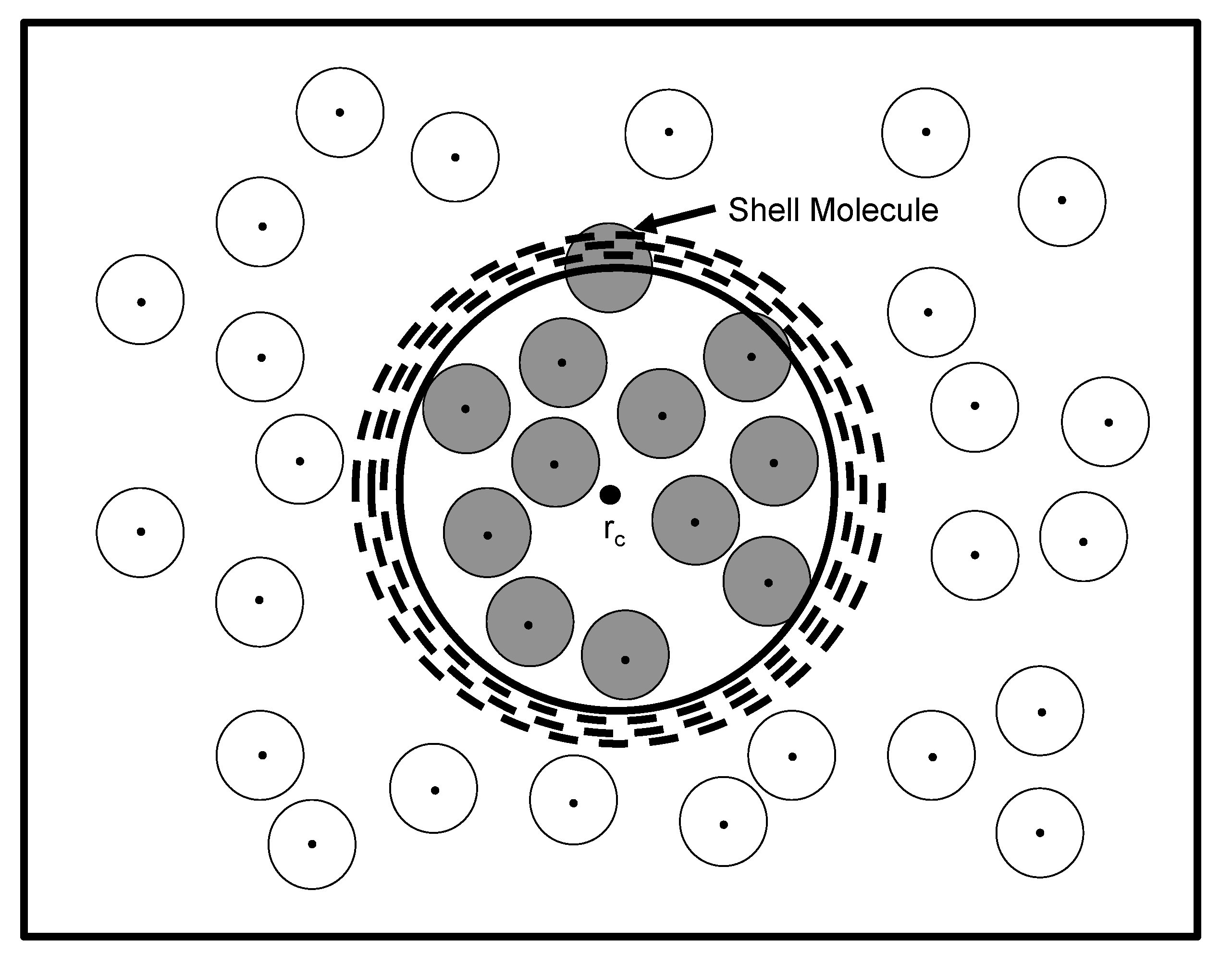The problem of over-counting is removed by requiring that the volume, V, of the system be specified by a “shell” molecule, where at least one molecule resides in the volume, $dV$, surrounding V. To illustrate this problem, turn to Figure 1, which demonstrates how several volumes may enclose the same configuration of n particles surrounded by $N-n$ particles. In the rigorous formulation of the $NPT$ ensemble, each configuration of the system must correspond to only one specific volume state of the n particles. Otherwise, the same configuration will be counted more than once in Equation (2) [14]. The problem of over-counting, or redundancy, is resolved by defining a “shell” particle [12,13,14], in which at least one of the system particles resides in the shell that encapsulates the system volume. Defining the n-particle system with the shell particle means that a new and distinct state of the total N-particle system is necessarily created when the volume of the n-particle system is varied (whether or not the configuration of the surrounding $N-n$ particles changes), since the position of the shell particle changes, as well [14]. Consequently, the inclusion of configurations of the n particles common to larger values of the volume is explicitly avoided.

Figure 1. One particular configuration of N particles enclosed within a total volume, V, demonstrating how to uniquely define one specific volume state of n particles (shaded circles). The unshaded circles represent the surrounding $N-n$ particles that comprise the bath. Each particle center is marked by a dot and is surrounded by an effective diameter. The first step in determining the volume occupied by the n particles is to choose a particular reference point in V as the origin, $r_c$. Yet, several volumes (dashed circles) centered at $r_c$ still enclose the n particles and, therefore, include common configurations. The exact volume, v (bold circle), of the n particles is defined by the presence of a shell particle that is farthest from $r_c$ and resides in the shell, $dv$, encapsulating v. (Adapted from Figure 2 in reference [14].)

Figure 1. One particular configuration of N particles enclosed within a total volume, V, demonstrating how to uniquely define one specific volume state of n particles (shaded circles). The unshaded circles represent the surrounding $N-n$ particles that comprise the bath. Each particle center is marked by a dot and is surrounded by an effective diameter. The first step in determining the volume occupied by the n particles is to choose a particular reference point in V as the origin, $r_c$. Yet, several volumes (dashed circles) centered at $r_c$ still enclose the n particles and, therefore, include common configurations. The exact volume, v (bold circle), of the n particles is defined by the presence of a shell particle that is farthest from $r_c$ and resides in the shell, $dv$, encapsulating v. (Adapted from Figure 2 in reference [14].)

Therefore, the proper form of $\Delta (N,P,T)$, in which interactions between the system and surroundings are neglected, as in Equation (2), should be [12,13,14]:

$$\begin{array}{ccc}\hfill \Delta (N,P,T)& =& {\int }_0^{\infty }{Q}^{*}(N,V,T)e^{-PV/k_{B}T}dV\hfill \end{array}$$

(4)

where $Q^{*}(N,V,T)dV$ represents the number of configurations in which at least one of the N particles resides in the shell, $dV$, surrounding V. Note that the above partition function is dimensionless, since $Q^{*}(N,V,T)dV$ is a pure number (or $Q^{*}(N,V,T)$ is a density of states). The shell particle is the correct volume scale when there is not a physical boundary to attach the volume of the system. Koper and Reiss [12] demonstrated that the states summed in Equation (4) do not contain common configurations, because the shell particle sets the volume. As shown above, all redundancies are eliminated by equating the system volume to the shell molecule.

2.1. Cubic System Volume

The application of the constant pressure ensemble to small systems also reveals the effects of additional variables, such as surface area and curvature, on the system’s properties. In the thermodynamic limit, the shape of the container enclosing the system has no influence on its properties. As the size of the system is decreased, additional independent thermodynamic variables (e.g., surface area, curvature) must be introduced to ensure that the system’s properties are described properly. These additional parameters are a function of the “shape” of the system volume. Therefore, the constant pressure ensemble partition function must be formulated differently in order to describe a system in which its volume is always either spherical (e.g., physical cluster) or cubic (the standard shape used to apply periodic boundary conditions). As a result, ensemble averages within the constant pressure ensemble will depend upon the shape of the system volume. This dependence upon shape, of course, becomes negligible in the thermodynamic limit. A reader interested in spherical systems is referred to [15]. However, since we are focusing on MD simulations with periodic boundary conditions, we are going to present results for a cubic volume [15].

The mathematical representation of $Q^{*}(N,V,T)dV$ for a cubic volume, $V=L^3$, whose length, L, lies between L and $L+dL$ with at least one particle in the shell, $dL$, is given by [15,16,17,18]:

$$\begin{array}{ccc}\hfill Q_{cub}^{*}(N,L,T)dL& =& \frac{3dL}{(N-1)!{\Lambda }^{3N}}{\int }_{A}d{y}_{1}d{z}_1{\int }_{V^{N-1}}d{\tau }_{12}...d{\tau }_{1N}{e}^{-\beta U_N}\hfill \end{array}$$

(5)

where $\beta =1/k_{B}T$, Λ is the de Broglie wavelength, A represents the area of a face of the cube, $d{y}_1$ and $d{z}_1$ represent the differential change in the y and z coordinates of particle 1 (the shell particle), respectively, ${\tau }_{12}...{\tau }_{1N}$ are the coordinates of the remaining $N-1$ particles relative to the position of particle 1, and $U_N$ is the interaction potential of all the N particles. The number three is required by the switch from $dV$ to $3L^{2}dL$, since volume changes occur with constant shape, and indicates the three sets of equivalent configurations generated if a particle is held fixed in the shell in either the x, y or z direction. Particle 1 cannot be integrated throughout the entire shell, but due to symmetry, can be integrated separately in the x direction (or the y or z direction). The above integral is therefore evaluated with the x coordinate of particle 1 held fixed in the plane that corresponds to one of the two faces of the cube perpendicular to the x-axis of the coordinate system.

With Equation (5), the isothermal-isobaric ensemble partition function for a cubic volume is now represented by [15,16,17,18]:

$${\Delta }_{cub}(N,P,T)=\int Q_{cub}^{*}(N,L,T)e^{-P{L}^3/k_{B}T}dL$$

(6)

Within the $NPT$ ensemble, the instantaneous pressure, $P^{″}$, of the system fluctuates. The instantaneous pressure is defined as [15,16,17,18]:

$$\begin{array}{ccc}\hfill P^{″}& =& \frac{k_{B}T}{3L^2}{\left(\frac{\partial ln{Q}_{cub}^{*}}{\partial L}\right)}_{T,N}\hfill \end{array}$$

(7)

and is calculated during a simulation via the following equation [15]:

$$\begin{array}{ccc}\hfill P^{″}& =& \frac{(N-1/3)k_{B}T}{V}+\frac{\langle {\sum }_i{\sum }_{j>i}{\overrightarrow{r}}_{ij}·{\overrightarrow{f}}_{ij}\rangle }{3V}\hfill \end{array}$$

(8)

where the second term on the right side is the standard virial of the system, ${\overrightarrow{r}}_{ij}$ is the vector between the centers of particles i and j and ${\overrightarrow{f}}_{ij}$ is the corresponding force. The ideal, or kinetic, term now reflects the loss of one, out of $3N$, translational degree of freedom. By defining the system volume and, therefore, being directly coupled to the barostat via the changes in the volume, the shell particle does not translate freely, that is, independently of the volume, in the x direction and, so, does not impart any momentum in the x direction to the surface of the cube. The shell particle translates freely in only two directions (y and z). The virial term in Equation (8) remains unchanged, since the shell particle still interacts with the other particles in the system. The ensemble average of $\langle P^{″}\rangle$ is related to the externally imposed pressure, P, as follows [15]:

$$\langle P^{″}\rangle =P+\frac{2k_{B}T}{3N}\langle \rho \rangle$$

(9)

where $\langle \rho \rangle$ is the average density of the system.

While revising the Monte Carlo $NPT$ algorithm to incorporate the shell particle, Corti [15] derived several relations that describe how ensemble averages obtained within the new $NPT$ partition function, Equation (4) or (6), relate to ensemble averages obtained with the old no-shell $NPT$ (Equation (2)) partition function, ${\Delta }_0$, [15]. If $\langle V\rangle$ represents the ensemble-averaged volume defined via the shell particle and ${\langle V\rangle }_0$ represents the ensemble-averaged volume defined via the old definition, then [15]:

$$\begin{array}{ccc}\hfill \langle V\rangle & =& {\langle V\rangle }_0-\frac{k_{B}T}{P}\hfill \end{array}$$

(10)

Consequently, $\langle V\rangle <{\langle V\rangle }_0$; the difference between these two average volumes is only apparent at small system sizes, since in the thermodynamic limit, $\langle V\rangle \to {\langle V\rangle }_0$ ($k_{B}T/P$ is intensive).

2.2. Ideal Gas Results

The ideal gas offers a unique opportunity to obtain a closed form solution for the partition function. Using the shell molecule definition (Equation (4)), we obtain [14]:

$$\begin{array}{c}\hfill \Delta (N,P,T)={\int }_0^{\infty }{Q}_{id}^{*}(N,V,T)e^{-\beta PV}dV={\int }_0^{\infty }\frac{V^{N-1}}{(N-1)!{\Lambda }^{3N}}{e}^{-\beta PV}dV={\left(\frac{1}{\beta P{\Lambda }^3}\right)}^N\end{array}$$

(11)

Using the following definition [31,32]:

$$\begin{array}{c}\hfill \langle V\rangle =-k_{B}T{\left(\frac{\partial ln\Delta }{\partial P}\right)}_{\beta ,N}\end{array}$$

(12)

we get the following expression for the equation of state [14]:

$$\begin{array}{c}\hfill P\langle V\rangle =N{k}_{B}T\end{array}$$

(13)

Now, we can use the older partition function (Equation (2)) and perform the same analysis. The partition function is [14]:

$$\begin{array}{c}\hfill {\Delta }_0(N,P,T)=\frac{1}{V_0}{\int }_0^{\infty }{Q}_{id}(N,V,T)e^{-\beta PV}dV=\frac{1}{V_0}{\int }_0^{\infty }\frac{V^N}{\left(N\right)!{\Lambda }^{3N}}{e}^{-\beta PV}dV=\frac{1}{V_0}\frac{1}{{\Lambda }^{3N}{\left(\beta P\right)}^{N+1}}\end{array}$$

(14)

We then get the following equation of state, noting that $V_0$ is a constant [14]:

$$\begin{array}{c}\hfill P{\langle V\rangle }_0=(N+1)k_{B}T\end{array}$$

(15)

The use of ($N+1$) or N is clearly inconsequential in the thermodynamic limit. Yet, the difference between Equations (13) and (15) is significant when the system is sufficiently small. In general, the ensemble averages calculated within different ensembles will not be the same for small systems. In contrast, ensemble averages are independent of the particular ensemble chosen to evaluate them when the system is in the thermodynamic limit. One exception, however, is the ideal gas. Due to the absence of inter-particle interactions, identical results should be obtained within all ensembles and for all system sizes. Hence, the small system $NPT$ partition function of the ideal gas should yield Equation (13) and not Equation (15).

3. Shell Molecule Equations of Motion

In order to simulate the $NPT$ ensemble, a technique for maintaining a constant temperature needs to be introduced into the equations of motion. As mentioned earlier, Nosé [2,3] and Hoover [4] proposed a completely dynamic method for maintaining constant temperature in an MD simulation. An additional variable, which serves to couple the system to a thermostat of fixed temperature T, is added to the Lagrangian of the N-body system. An effective mass is then associated with this new variable and controls the time scale for temperature fluctuations. While this scheme is usually effective, it does not always perform well [23]. In some cases, the resulting equations of motion do not generate phase-space trajectories that are ergodic [4]. To overcome this potential problem, the Nosé- Hoover chain method [23] was later developed. In this method, multiple thermostats are themselves successively coupled to adjacent thermostats, thereby forming a chain of thermostats.

The equations of motion for the $NPT$ ensemble with the shell particle are straightforwardly obtained by employing an extended Lagrangian approach. The full derivation is presented in appendix A of reference [16]. For a cubic volume in which $V=L^3$, we let the $+x$ coordinate of particle 1, or the shell particle, define half the box length, $L/2$, of the simulation cell. We also choose $q_i$ and $p_i$ to represent the $3N$-generalized coordinates and conjugate momenta, respectively. Note that we always have that $q_1=L/2$. We therefore get the following equations of motion for an isothermal-isobaric ensemble consistent with Equation (6) using a single thermostat chain for all of the particles [16]:

$$\begin{array}{ccc}\hfill {\dot{q}}_i& =& \frac{p_i}{m_i}+\left(\frac{{\dot{q}}_1}{q_1}\right)q_i\hfill \\ \hfill {\dot{p}}_i& =& F_i-\left(\frac{{\dot{q}}_1}{q_1}\right)p_i-{\dot{\xi }}_1{p}_i\hfill \\ \hfill {\dot{q}}_1& =& \frac{p_1}{m_1}\hfill \\ \hfill {\dot{p}}_1& =& 24q_1^2(P_{int}-P)-{\dot{\xi }}_1{p}_1\hfill \\ \hfill {\dot{\xi }}_k& =& \frac{p_{{\xi }_k}}{Q_k}\hfill \\ \hfill {\dot{p}}_{{\xi }_1}& =& \sum _{j=1}^{3N}\frac{p_j^2}{m_j}-{\dot{\xi }}_2{p}_{{\xi }_1}-g{k}_{B}T\hfill \\ \hfill {\dot{p}}_{{\xi }_k}& =& \frac{p_{{\xi }_{k-1}}^2}{Q_{k-1}}-\left({\dot{\xi }}_{k+1}\right)p_{{\xi }_k}-k_{B}T\hfill \\ \hfill {\dot{p}}_{{\xi }_C}& =& \frac{p_{{\xi }_{C-1}}^2}{Q_{C-1}}-k_{B}T\hfill \end{array}$$

(16)

where $i=2,...,3N$, and the overdots signify time derivatives. $F_i$ is the x, y or z component of the force acting on the particle represented by the ith-generalized coordinate, and $m_i$ is the corresponding mass of the particle. Each ${\xi }_k$ is a thermodynamic friction coefficient introduced to simplify the equations, and $p_{{\xi }_k}$ is the corresponding momentum of ${\xi }_k$, whose effective mass is $Q_k$. C is the total number of coupled thermostats in the chain, so that $k=1,...,C$, and g denotes the total number of degrees of freedom of the momenta of the particles. The expression for the internal pressure, $P_{int}$, which follows from Equation (6), is:

$$P_{int}=\frac{1}{24q_1^3}\left[\sum _{i=2}^{3N}\frac{p_i^2}{m_i}+\sum _{i=1}^{3N}{q}_i{F}_i\right]$$

(17)

where the first summation runs from two to $3N$, indicating that the x momentum of the shell particle does not contribute to the internal pressure.

The extended Hamiltonian, $H_{ext}$, for this system is [16,17,18]:

$$\begin{array}{c}\hfill H_{ext}=\sum _{i=1}^{3N}\frac{p_i^2}{2m_i}+\sum _i\sum _{j>i}U\left(r_{ij}\right)+8q_1^{3}P+\sum _{k=1}^C\frac{p_{{\xi }_k}^2}{2Q_k}+g{k}_{B}T{\xi }_1+\sum _{k=2}^C{k}_{B}T{\xi }_k\end{array}$$

(18)

where $V=8q_1^3$, $U\left(r_{ij}\right)$ is the interaction potential between particles i and j and ${\sum }_i{\sum }_{j>i}$ is a sum over all distinct pairs of particles. Although the equations of motion cannot be obtained directly from Equation (18), $H_{ext}$ is a conserved quantity.

With the exception of those equations of motion that describe the velocity and acceleration of $q_1$, the proposed equations are the same as those of Andersen’s method [1]. The expression for the acceleration of $q_1$ provides an interesting physical interpretation. Given that the area of a single face of the simulation cell is $4q_1^2$ (since $L=2q_1$), the total surface area of the cube is $24q_1^2$. When multiplied by the difference between the internal and external pressures, we obtain the net force that drives the acceleration of $q_1$. This connection between the acceleration of $q_1$ and the pressure difference is more physically appealing than what appears in other methods [1,5,8]. Another benefit to the shell formulation is that the system itself sets the time scale for volume and pressure fluctuations, since the mass of the shell particle is known. In Andersen’s method, there is an unknown piston mass that sets the response time of volume and pressure fluctuations.

In the simulations performed in this work, the forces acting in the y and z directions on each particle sum to zero when there are no external forces in the y and z directions. The sum of forces in the x direction will not be zero, since the x directional momentum of the shell particle is directly coupled to the barostat. Therefore, only the linear momenta in the y and z directions are conserved. Furthermore, to avoid particle drift during simulations when periodic boundary conditions are applied, the center-of-mass momentum in the y and z directions is set equal to zero. Again, the center-of-mass momentum in the x direction is driven by the external pressure and cannot be held fixed at a zero value, though volume fluctuations ensure that the total momentum in the x direction averages to zero. Consequently, it can be shown that $g=3N-2$ [16,33], indicating that the above equations of motion yield trajectories in phase space that are consistent with a $(3N-2)PT$ partition function (there are $3N-2$ momentum degrees of freedom) [16].

The new equations of motion that employ a shell particle to define the system volume provide another example of a non-Hamiltonian system, in that Equation (16) cannot be derived from the extended Hamiltonian in Equation (18). A systematic procedure for extending classical statistical mechanics to non-Hamiltonian systems was proposed by Tuckerman et al. [6,34]. The crux of their analysis relies on the notion that non-Hamiltonian phase space is compressible, as opposed to its Hamiltonian counterpart. For a non-Hamiltonian system, the Jacobian describing the transformation from an initial phase-space vector to a phase-space vector at time t is not equal to unity. The invariant phase-space metric for a non-Hamiltonian system is therefore not the same as the Hamiltonian system. Nevertheless, using the procedure of Tuckerman et al. [6,34], where the compressibility of the phase space is taken into account, the extended system partition function can still be derived from the equations of motion and the various constraints, or conservation relations, on the system. The detailed phase space analysis of Equation (16) presented in reference [16] shows that the proposed shell particle equations of motion are completely consistent with the shell particle partition function (Equation (6)) with and without periodic boundary conditions.

3.1. The Hoover Algorithm and Periodic Boundary Conditions

The $NPT$ partition function in Equation (6) can be rewritten if the system is homogeneous and periodic boundary conditions are applied. Han and Son [35] showed that since periodic boundary conditions yield a transitionally symmetric system, particle 1 does not need to be held fixed inside the shell, $dL$. If all of the relative distances between the particles remain fixed, identical configurations will be generated if particle 1 is allowed to sample the entire instantaneous volume. Thus [15]:

$$\begin{array}{ccc}\hfill Q_{cub}^{*}(N,L,T)dL& =& \frac{3dL}{(N-1)!{\Lambda }^{3N}}{\int }_{A}d{y}_{1}d{z}_1{\int }_{V^{N-1}}d{\tau }_{12}...d{\tau }_{1N}{e}^{-\beta U_N}\hfill \\ & =& \frac{3dL}{(N-1)!{\Lambda }^{3N}}\frac{1}{L}{\int }_{V}d{\tau }_1...d{\tau }_N{e}^{-\beta U_N}=\frac{N}{V}Q(N,V,T)dV\hfill \end{array}$$

(19)

where $Q(N,V,T)$ is the canonical partition function without the shell molecule. Using Equation (19), we can write the isothermal-isobaric partition function as:

$$\begin{array}{ccc}\hfill {\Delta }_{PB}(N,P,T)& =& \int \frac{N}{V}Q(N,V,T)e^{-\beta PV}dV\hfill \end{array}$$

(20)

where the $PB$ subscript signifies that the partition function is only valid under the symmetry imposed by periodic boundary conditions [15,16]. This volume scale was derived earlier using the information theory by Attard [36].

Let us now consider the following equations of motion proposed for the $NPT$ ensemble by Hoover [4,5] with a single chained thermostat:

$$\begin{array}{ccc}\hfill {\dot{q}}_i& =& \frac{p_i}{m_i}+\left(\frac{\dot{V}}{3V}\right)q_i\hfill \\ \hfill {\dot{p}}_i& =& F_i-\left(\frac{\dot{V}}{3V}\right)p_i-{\dot{\xi }}_1{p}_i\hfill \\ \hfill \dot{V}& =& \frac{3p_{ϵ}}{M_p}V\hfill \\ \hfill {\dot{p}}_{ϵ}& =& 3V(P_{int}-P)-{\dot{\xi }}_1{p}_{ϵ}\hfill \\ \hfill {\dot{\xi }}_k& =& \frac{p_{{\xi }_k}}{Q_k}\hfill \\ \hfill {\dot{p}}_{{\xi }_1}& =& \sum _{j=1}^{3N}\frac{p_j^2}{m_j}+\frac{p_{ϵ}^2}{M_p}-{\dot{\xi }}_2{p}_{{\xi }_1}-g{k}_{B}T\hfill \\ \hfill {\dot{p}}_{{\xi }_k}& =& \frac{p_{{\xi }_{k-1}}^2}{Q_{k-1}}-\left({\dot{\xi }}_{k+1}\right)p_{{\xi }_k}-k_{B}T\hfill \\ \hfill {\dot{p}}_{{\xi }_C}& =& \frac{p_{{\xi }_{C-1}}^2}{Q_{C-1}}-k_{B}T\hfill \end{array}$$

(21)

where $i=1,...,3N$ and:

$$\begin{array}{c}\hfill P_{int}=\frac{1}{3V}\left[\sum _{i=1}^{3N}\frac{p_i^2}{m_i}+\sum _{i=1}^{3N}{q}_i{F}_i\right]\end{array}$$

(22)

The extended Hamiltonian for the Hoover $NPT$ algorithm is:

$$\begin{array}{c}\hfill H_{ext}=\sum _{i=1}^{3N}\frac{p_i^2}{2m_i}+\sum _i\sum _{j>i}U\left(r_{ij}\right)+\frac{p_{ϵ}^2}{2M_P}+PV+\sum _{k=1}^C\frac{p_{{\xi }_k}^2}{2Q_k}+g{k}_{B}T{\xi }_1+\sum _{k=2}^C{k}_{B}T{\xi }_k\end{array}$$

(23)

Tuckerman et al. [6] already performed the phase-space analysis on Hoover’s equations of motion, in which they obtained a $1/V$ weighting in the volume distribution function when all three directional linear momenta are conserved, as well as the three center-of-mass momenta being set to zero. The appearance of the $1/V$ weighting of the volume distribution makes it completely consistent with the partition function introduced by Attard (Equation (20)). The Hoover algorithm does in fact lead to the correct sampling of volume states, but only for homogenous systems with periodic boundary conditions. In the absence of external forces, Hoover’s algorithm yields a $(3N-2)PT$ ensemble: there are a total of $(3N+1)$ momentum degrees of freedom ($3N$ particles and one volume), but now, the total linear momentum in each of the three directions is conserved. Therefore, $g=3N-2$ in Equation (21).

Although the Hoover algorithm does sample phase space correctly (but only for periodic boundary conditions), there is still an unknown piston mass, which sets the response time of volume and pressure fluctuations, which must be specified. On the other hand, when the shell particle formulation is used, the system itself sets the time scale for volume and pressure fluctuations, since the mass of the shell particle is known. Furthermore, since the piston mass associated with the Hoover algorithm can have very different dynamics compared to the particles in the system, it is the suggested form of the equations of motion to use two separate chained thermostats, one coupled to the particles and the other to the volume [8]. The need to introduce another set of chained thermostats to drive the volume fluctuations in the Hoover algorithm requires that another set of unknown parameters, the additional thermostat masses, be specified [8]. This separate thermostat chain is not necessary with the shell particle algorithm, as the momentum of the shell particle is on the same scale as the rest of the particles of the system [16,17].

As a final point of interest and, again, to focus on the effects of the different barostats, we briefly consider the results of the phase-space analysis of the $NPT$ equations of motion for the shell (Equation (16)) and the Hoover algorithm (Equation (21)). The explicit partition functions are derived in reference [16], where the influence of each barostat is clearly seen. By definition, the enthalpy, H, of the system is equal to $H=H(q,p)+PV$, where $H(p,q)={\sum }_{i=1}^{3N}{p}_i^2/2m_i+U\left(q\right)$. Hoover’s algorithm generates an extended Hamiltonian (Equation (23)) that contains an additional term associated with the kinetic energy of the volume ($p_{ϵ}^2/2M_P$), a quantity that should not appear in the enthalpy if the boundary used to describe the system volume is a mathematical construct to which a mass or momentum cannot be assigned [14]. In contrast, each configuration in the shell particle partition function corresponds to one and only one volume state, since the non-extended Hamiltonian is directly coupled to the volume (i.e., there is a one to one correspondence with the non-extended Hamiltonian and the volume states) [16]. The redundant counting of volume states is not eliminated in the other algorithms, because those non-extended Hamiltonians are decoupled from the volume. Note that whenever we use the extended variables approach to thermostat systems in this manuscript that there is always a kinetic term associated with the thermostat variables in the extended Hamiltonian. We are focusing here on how the positions and momenta are sampling the correct distribution, and the preceding argument on the enthalpy is independent of this kinetic term, due to the thermostat variables.

We conclude this section by noting that the ensemble average pressure for a system whose partition function is described by Equation (20) obeys the following relation [15]:

$$\begin{array}{ccc}\hfill \langle P^{″}\rangle & =& P+\frac{k_{B}T}{N}\langle \rho \rangle \hfill \end{array}$$

(24)

The correction to the ensemble average volume is the same as is given in Equation (10).

3.2. Multicomponent Systems

In this section, we discuss the extension of the shell particle MD algorithm to multicomponent systems. In particular, we consider a binary mixture comprised of species A and B. In this case, the isothermal-isobaric partition function must include configurations in which the shell particle is of type A and configurations in which the shell particle is of type B. Therefore, the isothermal-isobaric partition function, ${\Delta }_{AB}$, is given by (only the case of a cubical volume is considered) [15,17]:

$$\begin{array}{ccc}\hfill {\Delta }_{AB}(N,P,T)& =& \int Q_{cub}^{*A}(N,V,T)e^{-\beta P{L}^3}dL+\int Q_{cub}^{*B}(N,V,T)e^{-\beta P{L}^3}dL\hfill \end{array}$$

(25)

where $Q_{cub}^{*A}(N,V,T)$, for example, is the total number of configurations of $N_A$ particles of type A and $N_B$ particles of type B contained in a volume $V=L^3$ in which at least one of the $N_A$ particles resides in the shell, $dL$, encapsulating V.

When periodic boundary conditions are applied, one can show that the probability of a given configuration having a shell particle of type A is simply equal to the mole fraction of A. Begin with the partition function, ${\Delta }_A$, that includes only those configurations in which the shell particle is of type A:

$$\begin{array}{ccc}\hfill {\Delta }_A(N,P,T)& =& \int Q_{cub}^{*A}(N,V,T)e^{-\beta P{L}^3}dL\hfill \end{array}$$

(26)

For a homogeneous fluid in which periodic boundary conditions are employed, one can rewrite ${\Delta }_A$, following the argument presented by Han and Son [35], as:

$$\begin{array}{ccc}\hfill {\Delta }_A(N,P,T)& =& N_A\int \frac{Q(N,V,T)}{V}{e}^{-\beta PV}dV\hfill \end{array}$$

(27)

where $Q(N,V,T)$ is the canonical ensemble partition function for $N_A$ and $N_B$ particles without a shell particle used to define the volume. The fraction of configurations containing a shell particle of type A is therefore given by $N_A/(N_A+N_B)=x_A$ [17]. It was shown in reference [17] that the ensemble average of F (F being any given quantity) is given by:

$$\langle F\rangle =x_A{\langle F\rangle }_A+x_B{\langle F\rangle }_B$$

(28)

where ${\langle F\rangle }_A$ is the ensemble average obtained with only A as the shell particle and ${\langle F\rangle }_A$ is the ensemble average obtained with only B as the shell particle. Hence, two separate simulations can be run, each with different identities of the shell particle, with the resulting ensemble averages simply weighted by the mole fractions of each component. Yet, one can proceed even further and demonstrate that only one simulation per state point is ultimately required, with the identity of the shell particle being completely arbitrary. With periodic boundary conditions, we showed in reference [17] that $\langle F\rangle ={\langle F\rangle }_A={\langle F\rangle }_B$. Therefore, only one single simulation is required; the choice of which species to be the shell particle is solely a matter of convenience [17]. This conclusion also holds for mixtures with more than two components, again, only when periodic boundary conditions are employed.

3.3. Collision Dynamics for Discontinuous Potentials

In this section, we discuss the implementation of the shell particle formalism to simulate systems that have discontinuous intermolecular potentials [18]. Discontinuous molecular dynamics (DMD) have been widely used for quite some time, beginning with the initial work of Alder and Wainwright [37,38] in the microcanonical ensemble. Gruhn and Monson [39], following an analysis by de Smedt et al. [40], extended DMD for the hard-sphere potential to the $NPT$ ensemble. Their method, however, was based on Andersen’s constant pressure algorithm [1], which does not yield averages consistent with Equation (6). Gruhn and Monson [39] derived expressions for the discontinuous change of the momenta of two hard spheres upon collision, as well as the change of the velocity of the piston (or system volume) upon that same collision.

We use the shell particle equations of motion provided in Equation (16) to develop a constant pressure DMD algorithm for both the hard-sphere and square-well fluids that are consistent with the proper $NPT$ ensemble partition function, Equation (6). Momentum changes upon the collision of any two particles, including those changes for the shell particle, whether or not it participates in the collision, were derived in reference [18] and presented below. Our method is based on that of Gruhn and Monson [39], though we utilize the conservation of the extended Hamiltonian to obtain the collision dynamics. We simply present the results below, so the reader interested in the detailed derivations are referred to [18].

In an additive hard-sphere system, the potential of interaction between two particles, i and j, with diameters, ${\sigma }_i$ and ${\sigma }_j$, respectively, is represented by:

$$\begin{array}{c}\hfill u\left(r\right)=\left\{\begin{array}{cc}\infty ,\hfill & r<\sigma \hfill \\ 0,\hfill & r\ge \sigma \hfill \end{array}\right.\end{array}$$

(29)

where r is the distance between the particle centers and $\sigma =({\sigma }_i+{\sigma }_j)/2$. In between collisions, the hard-sphere fluid evolves dynamically without any force interactions. When applying the shell particle equations of motion to a hard-sphere collision, one must consider two separate cases: (1) neither particle i nor particle j is the shell particle and (2) either i or j is the shell particle. Furthermore, even if the shell particle does not participate in a collision, its x momentum will still change, since the acceleration of the shell particle is proportional to the internal pressure, which varies upon any collision.

There are several variables that are present in all of the expressions for the collision dynamics. These are the reduced mass, μ, the center-to-center vector, $\overrightarrow{q}$, and $\dot{r}$. The reduced mass is

$$\begin{array}{c}\hfill \mu =\frac{m_i{m}_j}{m_i+m_j}\end{array}$$

(30)

where $m_i$ and $m_j$ are the masses of particles i and j, respectively. $\overrightarrow{q}$ is defined as $\overrightarrow{q}={\overrightarrow{q}}_i-{\overrightarrow{q}}_j$, and $\dot{r}$ is $\dot{r}=(\overrightarrow{q}·\dot{\overrightarrow{q}})/\sigma$, which is the time rate of change of $\overrightarrow{q}$ evaluated at $|\overrightarrow{q}|=\sigma$. When neither of the colliding particles are the shell particle, the collision dynamics are given by:

$$\begin{array}{ccc}\hfill {\overline{t}}_d& =& \frac{-2\mu \dot{r}}{1+\mu {\sigma }^2/m_1{q}_1^2}\hfill \\ \hfill \Delta {\overrightarrow{p}}_i& =& {\overline{t}}_d\frac{\overrightarrow{q}}{\sigma }\hfill \\ \hfill \Delta {\overrightarrow{p}}_j& =& -{\overline{t}}_d\frac{\overrightarrow{q}}{\sigma }\hfill \\ \hfill \Delta p_1& =& {\overline{t}}_d\frac{\sigma }{q_1}\hfill \end{array}$$

(31)

When one of the colliding particles is the shell particle, the collision dynamics are now given by:

$$\begin{array}{ccc}\hfill {\overline{t}}_d& =& \frac{-2\mu \dot{r}}{1+\mu {\sigma }^2/m_1{q}_1^2-\mu q_x^2/m_1{\sigma }^2}\hfill \\ \hfill \Delta {\overrightarrow{p}}_i& =& {\overline{t}}_d\frac{\overrightarrow{q}}{\sigma }\hfill \\ \hfill \Delta p_{1,y}& =& -{\overline{t}}_d\frac{q_y}{\sigma }\hfill \\ \hfill \Delta p_{1,z}& =& -{\overline{t}}_d\frac{q_z}{\sigma }\hfill \\ \hfill \Delta p_1& =& {\overline{t}}_d\frac{\sigma }{q_1}\hfill \end{array}$$

(32)

where, for example, $q_x$ is the x component of $\overrightarrow{q}$.

The square-well interaction potential is represented by:

$$\begin{array}{c}\hfill u\left(r\right)=\left\{\begin{array}{cc}\infty ,\hfill & r<\sigma \hfill \\ -ϵ,\hfill & \sigma \le r<\lambda \sigma \hfill \\ 0,\hfill & r\ge \lambda \sigma \hfill \end{array}\right.\end{array}$$

(33)

where λ is the width and ϵ is the depth of the square-well (and may vary depending upon the interaction between any two particles). The interaction at $r\to \sigma$ is identical to the hard-sphere collision obtained above. There are three other types of collisions that occur in the square-well system at $r\to \lambda \sigma$. The capture interaction is the case where i and j start beyond $\lambda \sigma$. There are two types of collision that occur at $\lambda \sigma$ when the starting distance between i and j are within the attractive well. The dissociation collision occurs when the molecules have enough kinetic energy to overcome the attractive potential energy and the molecules no longer interact, and the bounce collision occurs when there is not enough kinetic energy to overcome the attractive energy and the particle centers stay within the attractive well. The bounce dynamics are analogous to the hard-sphere collision presented above with the only difference being setting $\sigma =\lambda \sigma$ in Equations (31) and (32). The mathematical condition for determining if the collision is a bounce or a dissociation collision is that if $\mu {\dot{r}}^2/2\ge ϵ(1+\mu {\sigma }^2/m_1{q}_1^2)$ for the shell particle not taking part in the collision and $\mu {\dot{r}}^2/2\ge ϵ(1+\mu {\sigma }^2/m_1{q}_1^2-\mu q_x^2/m_1{\lambda }^2{\sigma }^2)$ when the shell particle is taking part in the collision, then the collision is a dissociation collision.

The collision dynamics for capture and dissociation differ only by a plus/minus sign, so we present them together. When neither of the colliding particles are the shell particle, the collision dynamics are given by:

$$\begin{array}{ccc}\hfill {\overline{t}}_d& =& \frac{\mu \dot{r}\pm \mu {[{\dot{r}}^2\pm (2ϵ/\mu )(1+\mu {\lambda }^2{\sigma }^2/m_1{q}_1^2)]}^{1/2}}{1+\mu {\lambda }^2{\sigma }^2/m_1{q}_1^2}\hfill \\ \hfill \Delta {\overrightarrow{p}}_i& =& -{\overline{t}}_d\frac{\overrightarrow{q}}{\lambda \sigma }\hfill \\ \hfill \Delta {\overrightarrow{p}}_j& =& {\overline{t}}_d\frac{\overrightarrow{q}}{\lambda \sigma }\hfill \\ \hfill \Delta p_1& =& -{\overline{t}}_d\frac{\lambda \sigma }{q_1}\hfill \end{array}$$

(34)

with the “+” being for capture and the “−” being for dissociation. When one of the colliding particles is the shell particle, then the collision dynamics are given by:

$$\begin{array}{ccc}\hfill {\overline{t}}_d& =& \frac{\mu \dot{r}\pm \mu {[{\dot{r}}^2\pm (2ϵ/\mu )(1+\mu {\lambda }^2{\sigma }^2/m_1{q}_1^2-\mu q_x^2/m_1{\lambda }^2{\sigma }^2)]}^{1/2}}{1+\mu {\lambda }^2{\sigma }^2/m_1{q}_1^2-\mu q_x^2/m_1{\lambda }^2{\sigma }^2}\hfill \\ \hfill \Delta {\overrightarrow{p}}_i& =& -{\overline{t}}_d\frac{\overrightarrow{q}}{\lambda \sigma }\hfill \\ \hfill \Delta p_{1,y}& =& {\overline{t}}_d\frac{q_y}{\lambda \sigma }\hfill \\ \hfill \Delta p_{1,z}& =& {\overline{t}}_d\frac{q_z}{\lambda \sigma }\hfill \\ \hfill \Delta p_1& =& -{\overline{t}}_d\frac{\lambda \sigma }{q_1}\hfill \end{array}$$

(35)

We integrate the $NPT$ equations of motion in between collisions via the application of the generalized Trotter expansion formula to the extended phase space classical Liouville operator discussed in the appendix and [17,18,22,24,41]. Since the thermostat variables have no influence on a hard-sphere or square-well collision, the updates of the thermostats can be completely decoupled from the updates of the particle positions and the momentum changes upon a collision. The full integration scheme is presented in detail in [18].

3.4. Shell Particle Simulations Using the Configurational Temperature

The concept of a configurational temperature was introduced in 1997 in the seminal paper by Rugh [42], which provided a tractable statistical mechanical expression for the reciprocal of this temperature. The expression for the configurational temperature was later generalized by Jepps et al. [43]. Since then, several MD algorithms have been developed that make use of the configurational temperature, but the few that are most useful for the current discussion are by Braga and Travis [44,45]. They introduced $NPT$ equations of motion that use the configurational temperature and showed the benefits of using this temperature, instead of the standard kinetic temperature, within nonequilibrium simulations [44,45].

The equations of motion that they derived are not consistent with the shell molecule partition function, however, and so, we reformulated their equations to account for this. The new equations of motion are:

$$\begin{array}{ccc}\hfill {\dot{q}}_i& =& \frac{p_i}{m_i}+\left(\frac{{\dot{q}}_1}{q_1}\right)q_i+\left(\frac{{\dot{q}}_1}{q_1}\right)(3N-1)\frac{F_i}{{\Delta }^{\prime }}+\dot{\xi }\frac{F_i}{{\Delta }^{\prime }}\hfill \\ \hfill {\dot{p}}_i& =& F_i\hfill \\ \hfill {\dot{q}}_1& =& \frac{p_1}{m_1}\hfill \\ \hfill {\dot{p}}_1& =& 24q_1^2(P_{int}-P)\hfill \\ \hfill \dot{\xi }& =& \frac{p_{\xi }}{Q}\hfill \\ \hfill {\dot{p}}_{\xi }& =& \sum _{i=2}^{3N}\frac{F_i^2}{{\Delta }^{\prime }}-k_{B}T\hfill \end{array}$$

(36)

where $i=2,...,3N$,

$$\begin{array}{c}\hfill {\Delta }^{\prime }=\sum _{i=2}^{3N}\left(\frac{{\partial }^{2}U}{\partial q_i^2}\right)\end{array}$$

(37)

where U is the total potential energy, and:

$$\begin{array}{ccc}\hfill P_{int}& =& \frac{1}{24q_1^3}\left[(3N-1)\sum _{i=2}^{3N}\frac{F_i^2}{{\Delta }^{\prime }}+\sum _{j=1}^{3N}{q}_j{F}_j\right]\hfill \end{array}$$

(38)

The extended Hamiltonian for the configurational temperature shell molecule system is:

$$\begin{array}{c}\hfill H_{ext}=\sum _{i=1}^{3N}\frac{p_i^2}{2m_i}+\sum _i\sum _{j>i}U\left(r_{ij}\right)+8q_1^{3}P+\frac{p_{\xi }^2}{2Q}+k_{B}T\xi \end{array}$$

(39)

The instantaneous configurational temperature, $k_B{T}_{conf}$, is:

$$\begin{array}{c}\hfill k_B{T}_{conf}=\sum _{i=2}^{3N}\frac{F_i^2}{{\Delta }^{\prime }}\end{array}$$

(40)

The instantaneous configurational temperature appearing in the above shell particle equations of motion differs from that of Braga and Travis [44,45], whereby the sums appearing in Equations (37) and (40) run from two to $3N$, as compared to one to $3N$. The x-component of the shell particle is not included in these summations, although the shell particle does still contribute to the forces (and their derivatives) of the remaining particles. Since the configurational temperature thermostating appears to be preferred in nonequilibrium simulations, as known artifacts seen in some simulations with the Nosé-Hoover thermostat were not exhibited with the configurational temperature thermostat [44,45], we also include below new results for $NPT$ MD simulations with the shell molecule using the configurational temperature.

4. Results and Discussion

Several tests of the new shell particle equations of motion (Equation (16)) have been published previously. The agreement between isobars predicted by the new shell molecule molecular dynamics, the shell molecule Monte Carlo algorithm [15] and the equation of state for the Lennard-Jones fluid introduced by Johnson et al. [46] is shown in Figure 1 of [17]. Similar agreement between the MD and MC results is presented in Figure 1 of [18] for the square-well potential, which also includes, for comparison, the predictions of an equation of state introduced by Patel et al. [47]. For both systems, the MD and MC simulation results agree with each other and with the appropriate equation of state to high accuracy over a very broad range of pressures. On the scale of the plots, the MD and MC results are nearly indistinguishable [17,18]. We also looked at the self-diffusion coefficients for various binary Lennard-Jones mixtures and compared them with results from MD simulations in the microcanonical ensemble [17]. The self-diffusion coefficients of each species were essentially identical within both ensembles.

The differences between systems that sample the rigorously correct volume distributions and those that do not can most readily be seen in small systems. Equations (9) and (10), for example, provide strict tests of the validity of the shell particle equations of motion when compared against simulation methodologies that don not employ the correct volume scale. Several state points for Lennard-Jones, hard-sphere and square-well fluids are compared in [17,18]. In each of the conditions studied, the relations derived earlier are found to be satisfied to a high accuracy. We also included results from the Hoover algorithm (Equation (21), where it is important to note that the internal pressure equation for the Hoover algorithm is given by Equation (24)).

As an additional test, we present here results for a pure component Lennard-Jones fluid with system sizes ranging from $N=16$ to 256. To avoid the use of long-range corrections, as well as force profiles that would not sum to zero in the y and z directions, we utilized the truncated and shifted force Lennard-Jones potential [38]:

$$\begin{array}{ccc}\hfill u\left(r\right)& =& 4ϵ\left[{\left(\frac{\sigma }{r}\right)}^{12}-{\left(\frac{\sigma }{r}\right)}^6\right]-u_{LJ}\left(r_c\right)-(r-r_c)u_{LJ}^{\prime }\left(r_c\right)\hfill \end{array}$$

(41)

where $r_c$ is the cutoff distance and $u_{LJ}^{\prime }\left(r_c\right)$ is the derivative of the potential at the cutoff distance. At the chosen truncation distance, both the potential and force smoothly vanish. To prevent the truncation distance from exceeding half the box length at small system sizes, since periodic boundary conditions were employed, we chose $r_c=1.5\sigma$. Up to ${10}^6$ time steps of equilibration were performed, followed by up to ${10}^8$ time steps at the smallest system sizes for the determination of ensemble averages. All simulations were run at $T^{*}=1.5$. The results for a reduced external pressure of $P^{*}=0.5$ are included in Table 1. Additionally, provided in the tables are the averages obtained from MC simulations both with and without the shell particle.

Table 1. Comparison of various ensemble averages for the truncated and shifted Lennard-Jones fluid with a cuttoff of $1.5\sigma$ for $T^{*}=1.5$ and $P^{*}=0.5$. The top dataset was obtained with the shell particle Monte Carlo method [15]. The second dataset was generated from the shell particle molecular dynamics (MD) algorithm using the Nosé-Hoover chained thermostat. The third dataset was obtained from the shell particle MD algorithm using the configurational temperature thermostat. The fourth dataset was obtained from the Hoover algorithm. The bottom set are the results of constant pressure MC simulations without a shell particle. The numbers in parentheses indicate the error in the final significant digits.

N	$\langle {\mathit{P}}_{int}^{\mathbf{*}}\rangle$	$\langle {\mathit{\rho }}^{\mathbf{*}}\rangle$	$\langle {\mathit{V}}^{\mathbf{*}}\rangle$	$\langle {\mathit{U}}^{\mathbf{*}}\rangle$	$\langle {\mathit{T}}^{\mathbf{*}}\rangle$
16	0.514(54)	0.227(43)	73(7)	−0.045(32)	1.5
32	0.507(49)	0.223(34)	145(11)	−0.045(18)	1.5
64	0.503(37)	0.222(16)	291(14)	−0.045(12)	1.5
108	0.502(24)	0.221(8)	490(18)	−0.045(10)	1.5
256	0.501(15)	0.221(2)	1161(32)	−0.045(9)	1.5
16	0.514(235)	0.229(31)	72(12)	−0.045(111)	1.49(31)
32	0.506(161)	0.224(27)	144(17)	−0.045(78)	1.50(22)
64	0.503(111)	0.223(19)	290(25)	−0.045(55)	1.50(15)
108	0.502(85)	0.221(14)	489(32)	−0.045(42)	1.50(12)
256	0.501(55)	0.221(9)	1161(49)	−0.045(28)	1.50(8)
16	—	—	—	—	—
32	0.506(346)	0.218(27)	148(18)	−0.038(86)	1.51(15)
64	0.503(289)	0.219(21)	294(27)	−0.041(55)	1.51(14)
108	0.502(203)	0.219(15)	493(36)	−0.043(42)	1.50(12)
256	0.501(133)	0.220(9)	1165(50)	−0.044(28)	1.50(5)
16	0.522(235)	0.230(40)	71(12)	−0.047(111)	1.50(31)
32	0.511(162)	0.226(27)	144(17)	−0.045(78)	1.50(22)
64	0.505(111)	0.223(19)	289(24)	−0.045(55)	1.50(15)
108	0.503(85)	0.222(14)	488(32)	−0.045(42)	1.50(12)
256	0.501(56)	0.221(9)	1163(48)	−0.045(28)	1.50(8)
16	0.500(62)	0.220(18)	75(8)	−0.045(26)	1.5
32	0.500(44)	0.220(15)	147(11)	−0.045(18)	1.5
64	0.500(31)	0.220(10)	293(14)	−0.045(13)	1.5
108	0.500(25)	0.220(8)	492(20)	−0.045(8)	1.5
256	0.500(16)	0.220(2)	1164(36)	−0.045(5)	1.5

Table 1. Comparison of various ensemble averages for the truncated and shifted Lennard-Jones fluid with a cuttoff of $1.5\sigma$ for $T^{*}=1.5$ and $P^{*}=0.5$. The top dataset was obtained with the shell particle Monte Carlo method [15]. The second dataset was generated from the shell particle molecular dynamics (MD) algorithm using the Nosé-Hoover chained thermostat. The third dataset was obtained from the shell particle MD algorithm using the configurational temperature thermostat. The fourth dataset was obtained from the Hoover algorithm. The bottom set are the results of constant pressure MC simulations without a shell particle. The numbers in parentheses indicate the error in the final significant digits.

N	$\langle {\mathit{P}}_{int}^{\mathbf{*}}\rangle$	$\langle {\mathit{\rho }}^{\mathbf{*}}\rangle$	$\langle {\mathit{V}}^{\mathbf{*}}\rangle$	$\langle {\mathit{U}}^{\mathbf{*}}\rangle$	$\langle {\mathit{T}}^{\mathbf{*}}\rangle$
16	0.514(54)	0.227(43)	73(7)	−0.045(32)	1.5
32	0.507(49)	0.223(34)	145(11)	−0.045(18)	1.5
64	0.503(37)	0.222(16)	291(14)	−0.045(12)	1.5
108	0.502(24)	0.221(8)	490(18)	−0.045(10)	1.5
256	0.501(15)	0.221(2)	1161(32)	−0.045(9)	1.5
16	0.514(235)	0.229(31)	72(12)	−0.045(111)	1.49(31)
32	0.506(161)	0.224(27)	144(17)	−0.045(78)	1.50(22)
64	0.503(111)	0.223(19)	290(25)	−0.045(55)	1.50(15)
108	0.502(85)	0.221(14)	489(32)	−0.045(42)	1.50(12)
256	0.501(55)	0.221(9)	1161(49)	−0.045(28)	1.50(8)
16	—	—	—	—	—
32	0.506(346)	0.218(27)	148(18)	−0.038(86)	1.51(15)
64	0.503(289)	0.219(21)	294(27)	−0.041(55)	1.51(14)
108	0.502(203)	0.219(15)	493(36)	−0.043(42)	1.50(12)
256	0.501(133)	0.220(9)	1165(50)	−0.044(28)	1.50(5)
16	0.522(235)	0.230(40)	71(12)	−0.047(111)	1.50(31)
32	0.511(162)	0.226(27)	144(17)	−0.045(78)	1.50(22)
64	0.505(111)	0.223(19)	289(24)	−0.045(55)	1.50(15)
108	0.503(85)	0.222(14)	488(32)	−0.045(42)	1.50(12)
256	0.501(56)	0.221(9)	1163(48)	−0.045(28)	1.50(8)
16	0.500(62)	0.220(18)	75(8)	−0.045(26)	1.5
32	0.500(44)	0.220(15)	147(11)	−0.045(18)	1.5
64	0.500(31)	0.220(10)	293(14)	−0.045(13)	1.5
108	0.500(25)	0.220(8)	492(20)	−0.045(8)	1.5
256	0.500(16)	0.220(2)	1164(36)	−0.045(5)	1.5

According to Equation (10), the average volume of the shell particle simulations should be three units lower than the no-shell simulations in Table 1. The simulation results agree quite well with these predictions, considering the large absolute volume fluctuations that are obtained and satisfy Equation (10) with similar accuracy as noted in [15]. As expected, the average volume, density and internal energy per particle obtained with the shell particle MD with the traditional Nosé-Hoover thermostat, the shell particle MD with the configurational thermostat and the Hoover algorithms are in agreement, at least within the error bars. Both sets of averages are nearly the same for $P^{*}=0.5$. The average internal pressures differ, but each is seen to satisfy Equations (9) and (24) to a high degree of accuracy. Both of the shell particle results and Hoover results also agree, within the error bars, with the MC shell particle simulations. There is, however, a slight discrepancy between the MD and MC shell particle results at very small system sizes ($N\le 64$), particularly for the values of $P_{int}$ and the average density or volume. This difference can be attributed to the relatively large temperature fluctuations that develop within the MD simulations, as opposed to the strictly fixed temperature during the MC simulations. Statistical mechanics requires that the kinetic temperature of the system have a standard deviation of:

$${\sigma }_T=\sqrt{\langle T^2\rangle -{\langle T\rangle }^2}=T_{bath}\sqrt{\frac{2}{3N}}$$

(42)

where $T_{bath}$ is the temperature of the surrounding temperature reservoir and N is the number of particles in the system. Equation (42) holds regardless of the usage of periodic boundary conditions [25,33]. In Table 1, we report the standard deviation by the number in parentheses indicating the error in the final significant digits. As an example, the number $1.50\left(31\right)$ means that the average is calculated to be $1.50$ and the standard deviation is $0.31$. The results for the temperature fluctuations in Table 1 agree very closely to Equation (42).

Furthermore, presented in Table 1 are the results for the shell molecule configurational temperature $NPT$. Note that the results for the configurational temperature are not provided for $N=16$. At this small density and small number of particles, there is a chance that no pairs of particles reside within the cuttoff distance. As a result, ${\Delta }^{\prime }$ is equal to zero and the integration scheme breaks down for that time step. This problem only arose for the smallest system size ($N=16$). Additionally, note in Table 1 that the configurational temperature yields the largest temperature fluctuations as compared to the other simulation methods. Again, at this relatively low density, the effects of adding or deleting one or two particle pairs within the potential cutoff for each time step are greatly enhanced for the configurational temperature (as compared to the kinetic temperature, which is based solely on the particle momenta). The average volumes are larger than they should be and the average potential energy is lower than it should be for the configurational temperature simulations. Interestingly, the results do seem to improve consistently as the number of particles increases. This may be due, in some small part, to the given expression for the configurational temperature, which as a measure of the system temperature is only accurate on the order of ($1/N$) [44,45].

4.1. Discontinuous Pressure Jumps

Ultimately, the true benefits of the shell particle algorithm may become apparent for nonequilibrium simulations where the system itself sets the time scale for pressure/volume fluctuations. It is important to note that in a multicomponent system, there is freedom to choose the identity of the shell particle, although the masses of the various components comprising the mixture are still known. To gain some initial idea of how the shell particle equations of motion might behave in a nonequilibrium application, we ran a pressure-jump simulation in which the external pressure is abruptly changed after the system has equilibrated. For example, we first consider the response of the internal pressure to a sudden change in the external pressure from $P^{*}=1.0$ to $P^{*}=2.0$ and then back to $P^{*}=1.0$ at $T^{*}=2.0$ for the pure component Lennard-Jones fluid with $N=500$ and long-range corrections applied after a potential cutoff of $3.0\sigma$. 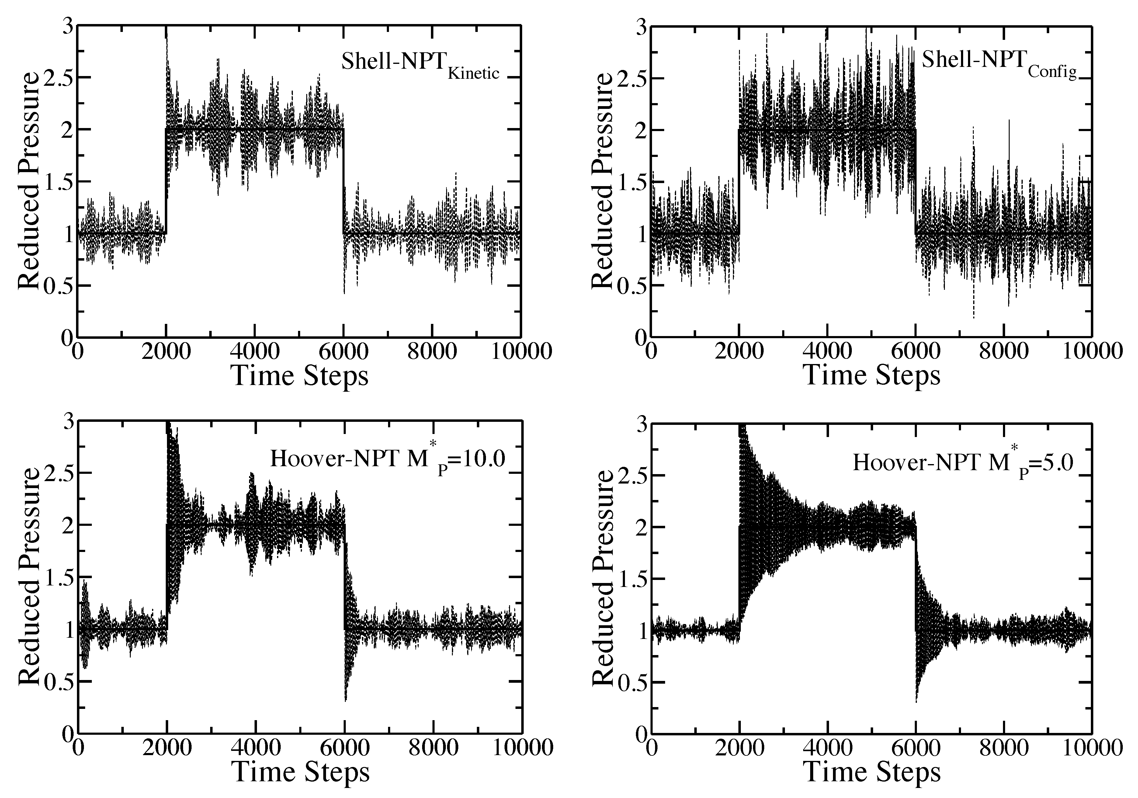The resulting time evolution of the internal pressure is shown in Figure 2.

Figure 2. Time response of the internal pressure of the pure component Lennard-Jones fluid to a sudden change of the external pressure from $P^{*}=1.0$ to $P^{*}=2.0$ and, then, back down to $P^{*}=1.0$. For the given choice of the time origin, the pressure is increased after 2000 time steps and, then, reduced after another 4000 time steps. The solid line is the set external pressure, P. The dashed lines are the simulation results. In all cases, $T^{*}=2.0$ and $N=500$. The plot in the upper-left corner is the results for the shell molecule with the Nosé-Hoover thermostat. The plot in the upper-right corner is the results for the shell molecule with the configurational temperature thermostat; The plots in the lower-left and lower-right corner are the results for the Hoover algorithm with $M_p^{*}=10.0$ and $M_p^{*}=5.0$, respectively.

Figure 2. Time response of the internal pressure of the pure component Lennard-Jones fluid to a sudden change of the external pressure from $P^{*}=1.0$ to $P^{*}=2.0$ and, then, back down to $P^{*}=1.0$. For the given choice of the time origin, the pressure is increased after 2000 time steps and, then, reduced after another 4000 time steps. The solid line is the set external pressure, P. The dashed lines are the simulation results. In all cases, $T^{*}=2.0$ and $N=500$. The plot in the upper-left corner is the results for the shell molecule with the Nosé-Hoover thermostat. The plot in the upper-right corner is the results for the shell molecule with the configurational temperature thermostat; The plots in the lower-left and lower-right corner are the results for the Hoover algorithm with $M_p^{*}=10.0$ and $M_p^{*}=5.0$, respectively.

The figure includes results for the shell molecule with the Nosé-Hoover thermostat, the shell molecule with the configurational temperature thermostat and results for the Hoover algorithm with the reduced piston mass, $M_p^{*}$, equal to $M_p^{*}=10.0$ and $M_p^{*}=5.0$, respectively. Both of the shell particle simulations and the Hoover simulation with $M_p^{*}=10.0$ quickly adjust to the new external pressure, while the Hoover simulation with $M_p^{*}=5.0$ requires a much longer time to re-equilibrate (again, the time scale obtained from the Hoover code is directly dependent upon the mass of the piston, whereas the time scale for the shell particle algorithm is automatically set by the system). This result is somewhat surprising, since the two piston masses are so close in their numerical values. The fluctuations of the internal pressure exhibited by both of the shell particle codes at the new external pressure of $P^{*}=2.0$ and, then, again, at $P^{*}=1.0$ are immediately identical to the fluctuations seen from regular equilibrium simulations at $P^{*}=2.0$ and $P^{*}=1.0$. The internal pressure for the Hoover simulations also adjusts to the new external pressure, but there does appear to be a considerable “decay” to the new set point after the pressure jump. This decay is dependent on the value of the piston mass. A smaller value of the piston mass yields a longer decay in the instantaneous pressure to the new equilibrium point.

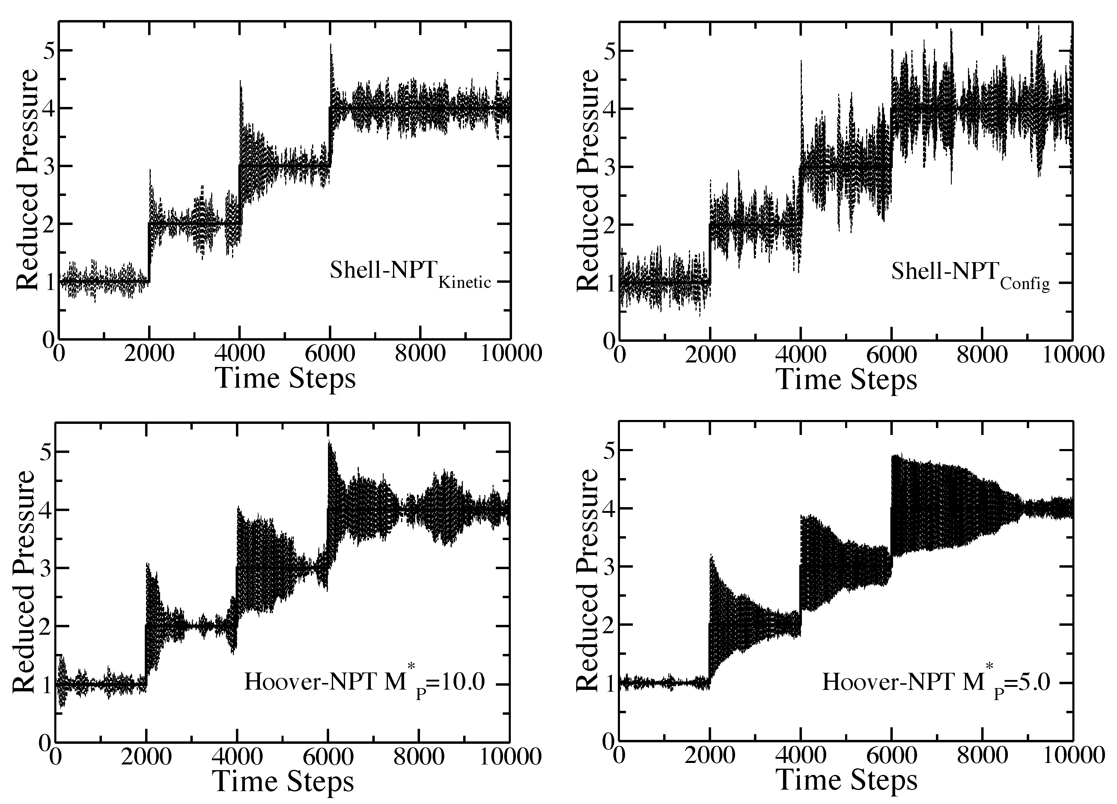
Figure 3. Time response of the internal pressure of the pure component Lennard-Jones fluid to an isothermal compression from $P^{*}=1.0$ to $P^{*}=4.0$ in increments of $1.0$ unit of reduced pressure every 2000 time steps. For the given choice of the time origin, the pressure is increased after 2000, 4000 and, again, after 6000 time steps. The solid line is the set external pressure, P. The dashed lines are the simulation results. In all cases, $T^{*}=2.0$ and $N=500$. The plot in the upper-left corner is the results for the shell molecule with the Nosé-Hoover thermostat. The plot in the upper-right corner is the results for the shell molecule with the configurational temperature thermostat. The plots in the lower-left and lower-right corner are the results for the Hoover algorithm with $M_p^{*}=10.0$ and $M_p^{*}=5.0$, respectively.

Figure 3. Time response of the internal pressure of the pure component Lennard-Jones fluid to an isothermal compression from $P^{*}=1.0$ to $P^{*}=4.0$ in increments of $1.0$ unit of reduced pressure every 2000 time steps. For the given choice of the time origin, the pressure is increased after 2000, 4000 and, again, after 6000 time steps. The solid line is the set external pressure, P. The dashed lines are the simulation results. In all cases, $T^{*}=2.0$ and $N=500$. The plot in the upper-left corner is the results for the shell molecule with the Nosé-Hoover thermostat. The plot in the upper-right corner is the results for the shell molecule with the configurational temperature thermostat. The plots in the lower-left and lower-right corner are the results for the Hoover algorithm with $M_p^{*}=10.0$ and $M_p^{*}=5.0$, respectively.

We also preformed an isothermal compression as a series of steps from $P^{*}=1.0$ to $P^{*}=4.0$ in increments of $1.0$ unit of reduced pressure every 2000 time steps at $T^{*}=2.0$ for the pure component Lennard-Jones fluid with $N=500$ and long-range corrections applied after a potential cutoff of $3.0\sigma$. The results are presented in Figure 3. The value of the time steps, along with every other aspect of the simulations, are the same as those performed for Figure 2. As before, both of the shell particle simulations exhibit fluctuations of the internal pressure after the jumps to be almost immediately identical to the fluctuations seen from regular equilibrium simulations at the respective set external pressures at equilibrium. The internal pressure for the Hoover simulations also adjust to the new external pressure, but again, there appears to be a considerable decay to the new set point after the pressure jump. The simulation with $M_P^{*}=5.0$ does not allow the internal pressure to equilibrate after an external pressure jump before the system takes the next jump. This shows that the value of the piston mass is critical to capturing the dynamics and fluctuations in nonequilibrium systems and that the results can be considerably different for values of the piston mass that are relatively close to one another.

5. Conclusions

The MD $NPT$ simulation method that employs the shell particle is based on equations of motion consistent with the proper statistical mechanical formulation of the $NPT$ ensemble. Within other MD methods, a piston of arbitrary mass is introduced to control the response time of volume fluctuations. Now, the shell particle of known mass determines the time scale for volume and pressure fluctuations, in addition to performing the important function of eliminating the redundant counting of configurations through its unique definition of the volume of the system.

There are several benefits to using the shell particle algorithm for MD equilibrium simulations. For example, as the shell particle directly interacts with all other particles in the system, only a single Nosé-Hoover chained thermostat need be employed. Additionally, as noted above, the mass of the “volume”, that is, the shell particle, is a known quantity.

Allowing the system itself to control the relaxation time of property fluctuations should ultimately provide a significant edge over piston-based methods, specifically for nonequilibrium systems (though that has yet to be shown). Adapting the shell particle approach to a simulation of isothermal-isobaric shear flow [44,45] or homogeneous nucleation in simple fluids [48,49,50] may provide another worthwhile test of the shell particle formalism. The piston mass is not known a priori and greatly affects the response time of the system. As such, for nonequilibrium simulations, the appropriate choice of a piston mass is unclear. On the other hand, at least for a pure component system, there is no ambiguity as to what should be the response time of the volume fluctuations; the mass of the shell particle is again a known input to the simulation. For mixtures, however, the identity of the shell particle is important (though not for equilibrium averages). Yet, the masses of the components comprising the mixture are still known. How the identity of the shell particle controls the response time of pressure and volume fluctuations is therefore, in the end, still a property of the system itself.

Future directions include incorporating the shell particle formalism into constant pressure molecular dynamics algorithms for both molecular systems and systems with long-range intermolecular interactions (such as electrostatic interactions). To date, we have not performed any simulations of these systems with the shell particle, so definitive statements would be inappropriate at this time. However, at first sight, it would appear that selecting the center of mass of one of the molecules as the volume scale is a logical choice for molecular systems. It also appears that the techniques already employed to deal with long-range interactions in previous algorithms (such as the Ewald summation in electrostatic systems) would apply equally to shell particle algorithms. There is nothing in the derivations given in this manuscript that suggests to us that intra- or long-range intermolecular interactions would have any effect on the validity of the shell molecule formulation.

Finally, various shape changing, or isotension, simulations [25] may also benefit from the use of the shell particle. The introduction of a shell particle into these codes would add some complexities, such as possibly allowing the shell particle to move along different faces of the system volume. Nevertheless, eliminating the need to specify a piston mass might be very helpful for these simulations.