Exact Probability Distribution versus Entropy

Department of Mathematics and Computer Science, Karlstad University, SE-651 88 Karlstad, Sweden
Entropy 2014, 16(10), 5198-5210; https://doi.org/10.3390/e16105198
Submission received: 26 May 2014
/
Revised: 20 September 2014
/
Accepted: 26 September 2014
/
Published: 7 October 2014
(This article belongs to the Section Information Theory, Probability and Statistics)
Abstract
:The problem addressed concerns the determination of the average number of successive attempts of guessing a word of a certain length consisting of letters with given probabilities of occurrence. Both first- and second-order approximations to a natural language are considered. The guessing strategy used is guessing words in decreasing order of probability. When word and alphabet sizes are large, approximations are necessary in order to estimate the number of guesses. Several kinds of approximations are discussed demonstrating moderate requirements regarding both memory and central processing unit (CPU) time. When considering realistic sizes of alphabets and words (100), the number of guesses can be estimated within minutes with reasonable accuracy (a few percent) and may therefore constitute an alternative to, e.g., various entropy expressions. For many probability distributions, the density of the logarithm of probability products is close to a normal distribution. For those cases, it is possible to derive an analytical expression for the average number of guesses. The proportion of guesses needed on average compared to the total number decreases almost exponentially with the word length. The leading term in an asymptotic expansion can be used to estimate the number of guesses for large word lengths. Comparisons with analytical lower bounds and entropy expressions are also provided.
1. Introduction
This work has been inspired by problems addressed in the field of computer security, where the attacking of, e.g., password systems is an important issue (see, e.g., [1] and [2]). In a brute-force attack, the password, for instance, can be broken in a worst-case time proportional to the size of the search space and, on average, a time half of that. However, if it is assumed that some words are more probable than others, the words can be ordered in the search space in decreasing order of probability. The number of guesses can then be drastically reduced. Properties of the average number of successive guesses have been discussed in detail by Pliam [3], who, to the best knowledge of the author, introduces the word guesswork to denote this quantity. Further, Lundin et al. [4] discuss confidentiality measures related to guesswork.
As will be demonstrated below, the calculation of the guesswork may require a substantial amount of computational effort, especially if the search space is large. Therefore lower bounds, which are easy to calculate, have been provided by several authors, e.g., Arikan [5] and Massey [6]. Lower and upper bounds are provided by Pliam [3], but they involve similar calculations as those needed for the guesswork itself and may therefore be of less practical use.
In this paper, numerical approaches are suggested for evaluating the average number of successive guesses (guesswork) required for correctly guessing a word from a given language. The guessing strategy used is guessing words in decreasing order of probability. This is a continuation of investigations presented elsewhere [7]. In Section 2, the languages used in this paper are presented together with the corresponding expressions for the guesswork and entropy. The reason for considering entropy here depends on the prevalent use of entropy instead of guesswork in applications due to its simpler determination. In Section 3, approximate numerical estimations of guesswork are discussed, and in Section 4, the results for some probability distributions are given. Finally, in Section 5, the conclusions of the investigations presented in the paper are summarized.
2. Languages
A language is a set of strings, and a string is a finite sequence of symbols from a given alphabet. Consider a stochastic variable X belonging to a state space
![Entropy 16 05198f5]() = {x1, x2,. . ., xn}, where the probability distribution is given by pX(x) = Pr(X = x). Introduce the short-hand notation pi = pX(xi), where
. In the following, the state space
= {x1, x2,. . ., xn}, where the probability distribution is given by pX(x) = Pr(X = x). Introduce the short-hand notation pi = pX(xi), where
. In the following, the state space
![Entropy 16 05198f5]() and its size n are considered as an alphabet with a certain number of symbols. Words are formed by combining symbols into strings. From n symbols, it is possible to form nm different words of length m. Shannon introduced various orders of approximations to a natural language, where the zero-order approximation is obtained by choosing all letters independently and with the same probability. In the first-order approximation, the complexity is increased by choosing the letters according to their probability of occurrence in the natural language. In zero- and first-order approximation, the strings thus consist of independent and identically-distributed (i.i.d.) random variables. For higher-order approximations, the variables are no longer independent [8].
and its size n are considered as an alphabet with a certain number of symbols. Words are formed by combining symbols into strings. From n symbols, it is possible to form nm different words of length m. Shannon introduced various orders of approximations to a natural language, where the zero-order approximation is obtained by choosing all letters independently and with the same probability. In the first-order approximation, the complexity is increased by choosing the letters according to their probability of occurrence in the natural language. In zero- and first-order approximation, the strings thus consist of independent and identically-distributed (i.i.d.) random variables. For higher-order approximations, the variables are no longer independent [8].
 = {x1, x2,. . ., xn}, where the probability distribution is given by pX(x) = Pr(X = x). Introduce the short-hand notation pi = pX(xi), where
. In the following, the state space
and its size n are considered as an alphabet with a certain number of symbols. Words are formed by combining symbols into strings. From n symbols, it is possible to form nm different words of length m. Shannon introduced various orders of approximations to a natural language, where the zero-order approximation is obtained by choosing all letters independently and with the same probability. In the first-order approximation, the complexity is increased by choosing the letters according to their probability of occurrence in the natural language. In zero- and first-order approximation, the strings thus consist of independent and identically-distributed (i.i.d.) random variables. For higher-order approximations, the variables are no longer independent [8].
= {x1, x2,. . ., xn}, where the probability distribution is given by pX(x) = Pr(X = x). Introduce the short-hand notation pi = pX(xi), where
. In the following, the state space
and its size n are considered as an alphabet with a certain number of symbols. Words are formed by combining symbols into strings. From n symbols, it is possible to form nm different words of length m. Shannon introduced various orders of approximations to a natural language, where the zero-order approximation is obtained by choosing all letters independently and with the same probability. In the first-order approximation, the complexity is increased by choosing the letters according to their probability of occurrence in the natural language. In zero- and first-order approximation, the strings thus consist of independent and identically-distributed (i.i.d.) random variables. For higher-order approximations, the variables are no longer independent [8].2.1. Zero-Order Approximation
In a zero-order approximation, all symbols in the alphabet (of size n) have the same probability of occurrence (pi = 1/n, ∀i = 1, . . ., n). The average number of guesses G0 required to correctly guess a word of length m is given by:
where H0(X1) = logb n and b is the base of the logarithm used. The average number of guesses grows exponentially with the size of the word, while the entropy grows linearly with the size of the word. This is in accordance with the definition of entropy, since it should be an extensive property growing linearly with the size of the system.
In a zero-order approximation, the relation between guesswork and entropy is G0(X1, . . ., Xm) = (bH0(X1,...,Xm) + 1)/2. This relationship between guesswork and entropy is true in zero-order approximation, but not necessarily so using higher-order approximations, which has been demonstrated by several authors (see, e.g., [3] and [9]). These authors strongly argue against the use of entropy in the estimation of the number of required guesses.
2.2. First-Order Approximation
In a first-order approximation, the symbols in the alphabet (of size n) do not necessarily have the same probability of occurrence. Assume the symbols are ordered in decreasing order of probability (p1 ≥ p2 ≥ . . . ≥ pn). In first order, the symbols in a word are considered as stochastically independent, and then, the most probable word (of a given length) would consist of only x1. The most improbable word, on the other hand, would consist of only xn. The average number of guesses G1 required for making the correct guess of a word of length m is given by the summation:
where the function g(i1, . . ., im) represents the number of guesses, one guess for the most probable word, two guesses for the second most probable word and nm guesses for the most improbable word, etc. The entropy H1 of a word of length m is given by [8]:
where b is the base of the logarithm used. The calculation of Equation (3) is more complicated than Equation (4), since it requires that the products of probabilities (pi1 · · · pim) are sorted in decreasing order. Such a procedure can be realized only for a moderate size of nm, due to both storage and CPU time requirements. For larger values of nm, approximate methods have to be used in order to get an estimate of the summation. Lower bounds of the guesswork, which are easy to calculate, have been provided by Massey [6] and Arikan [5]. Massey demonstrates that:
where b is the base of the logarithm used in H1, and Arikan that:
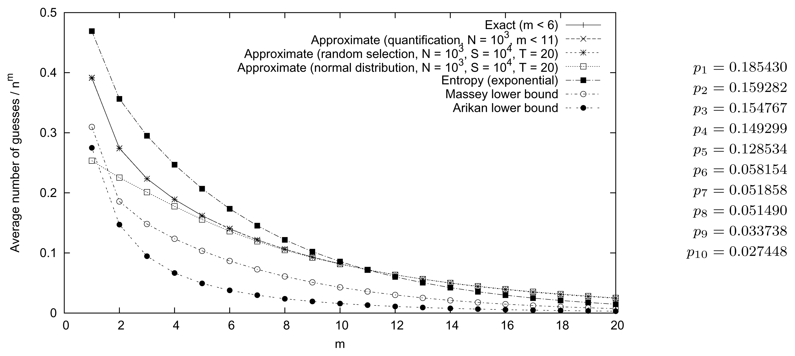
In Figure 1, the exact value of the guesswork for correctly guessing a word of size m < 6 using an alphabet of size 10 (with the randomly chosen probability distribution given in the figure) is displayed. The lower bounds provided by Equations (5) and (6) are given for word sizes m ≤ 20. For comparison, the exponential entropy expression, with the same functional form as guesswork in zero order (Equation (1)),
where b is the base of the logarithm used in H1, is given for word sizes m ≤ 20. For word sizes m < 6, Equation (7) clearly overestimates the exact value of the guesswork. In fact, Pliam has shown that it is possible to construct probability distributions that make guesswork differ arbitrarily much from Equation (7) [3]. In Section 3, approximate numerical evaluations of guesswork are discussed.
2.3. Second-Order Approximation
In a second-order approximation, the variables are no longer independent. Consider two jointly distributed stochastic variables X, Y ∈ ![Entropy 16 05198f5]() then, the conditional probability distribution of Y given X is given by pY (y|X = x) = Pr(Y = y|X = x). Introduce the short-hand notation Pij = pY (xj |X = xi), the probability that symbol xj follows symbol xi. P is an n × n matrix, where n is the size of the alphabet, and the sum of the elements in each row is one. The probability of occurrence of each symbol in the alphabet, pi, can easily be obtained from matrix P using the two equations (PT − I)p = 0 and |p| = 1, where p is a vector of length n with elements pi.
then, the conditional probability distribution of Y given X is given by pY (y|X = x) = Pr(Y = y|X = x). Introduce the short-hand notation Pij = pY (xj |X = xi), the probability that symbol xj follows symbol xi. P is an n × n matrix, where n is the size of the alphabet, and the sum of the elements in each row is one. The probability of occurrence of each symbol in the alphabet, pi, can easily be obtained from matrix P using the two equations (PT − I)p = 0 and |p| = 1, where p is a vector of length n with elements pi.
then, the conditional probability distribution of Y given X is given by pY (y|X = x) = Pr(Y = y|X = x). Introduce the short-hand notation Pij = pY (xj |X = xi), the probability that symbol xj follows symbol xi. P is an n × n matrix, where n is the size of the alphabet, and the sum of the elements in each row is one. The probability of occurrence of each symbol in the alphabet, pi, can easily be obtained from matrix P using the two equations (PT − I)p = 0 and |p| = 1, where p is a vector of length n with elements pi.The guesswork G2, i.e., the average number of guesses required for making the correct guess of a word of length m using an alphabet of size n, is given by:
where the function g(i1, . . ., im) is the same as the one in Equation (3). The entropy H2 of a word of length m is given by [10]:
where b is the base of the logarithm used. In Section 4, the value of Equation (8) will be compared to the value of Equation (7) (with H1 replaced by H2) for a given probability distribution.
3. Numerical Evaluation of Guesswork
In this section, a number of approaches will be given in order to evaluate the guesswork.
3.1. Quantification
One simple procedure for numerically estimating Equation (3) and in addition reducing the storage requirements is to split the range
into N equal pieces of size
, where a larger value of N gives a better estimate. The range
will consequently be split into m · N equal pieces of size Δ. Instead of sorting the products pi1pi2 · · · pim, they simply have to be evaluated and brought into one of the m · N subranges. When the number of products in each subrange has been determined, an estimate of Equation (3) can be made, giving:
where cj is the number of probability products in subrange j,
and
is the middle value of subrange j. By instead using the boundary values of the subranges, lower and upper bounds of the numerically-estimated guesswork can be given as:
where Q1 = (p1/pn)1/2N. Here, the short-hand notation Q1 is used instead of the more correct notation Q1(X1, . . ., Xm;N) in order to increase the transparency of Equation (11).
By introducing the density of products ρi = ci/(Δnm) (normalized to unity), the summations in Equation (10) can be replaced by integrals for large values of N, giving:
where b is the base of the logarithm used in ρ and Δ. Equation (12) will be of importance in Section 3.3, where a normal distribution approximation of the density of products is discussed.
The method of quantification can be used in both first- and second-order approximation. However, since it is less obvious in second order, which is the smallest and largest value of the product of probabilities pi1Pi1i2 · · · Pim−1im, a lower bound of min(pi) · min(Pij)m−1 and an upper bound of max(pi) · max(Pij)m−1 can be used instead to determine the range of possible values. When determining min(Pij), only non-zero values are considered. In second order, a similar expression as the one in Equation (11) can be used for estimating the guesswork, namely:
where
and
is given by Equation (10) using the values given above as interval limits for probability products. Here, the short-hand notation Q2 is used instead of the more correct notation Q2(X1, . . ., Xm;N) in order to increase the transparency of Equation (13).
3.2. Random Selection
The storage and CPU time requirements using the strategy in Section 3.1 for calculating the guesswork are of O(m · N) and O(m · nm), respectively. One simple modification for decreasing the time requirements is to reduce the number of probability products formed. Instead of calculating all nm different products, a smaller number of randomly chosen probability products is used and brought into the m · N subranges. The smaller number has been determined to be proportional to m, i.e., equal to m · S, where S is a parameter whose value has to be chosen. After normalization, where the number of products in each subrange is multiplied by the factor nm/(m · S), the strategy is identical to the one in Section 3.1.
By not using all nm different probability products, another error is introduced. This error can be estimated by repeating the random selection calculations a number of times (given by T). Through these calculations, an average value (
) and a standard deviation (
) can be estimated (where i = 1 or 2). A 99% confidence interval for
is then given as:
where
and λ0.01/2 = 2.58 (the quantile function of the normal distribution) [11]. In Equation (14), all parameters have been excluded in order to increase the transparency of the equation.
3.3. Normal Distribution
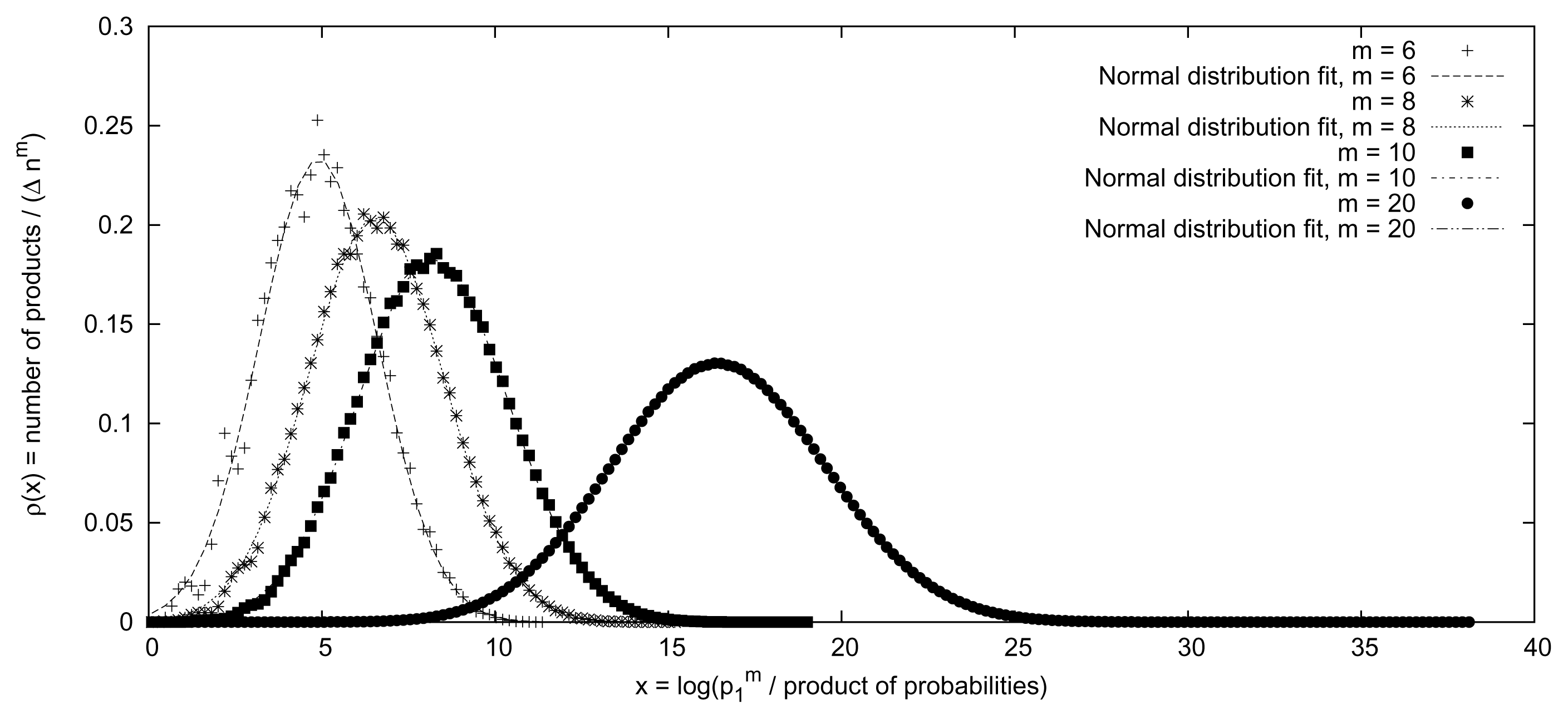
Another interesting approach is given by the central limit theorem in probability theory, which roughly states that the mean of a large number of independent stochastic variables is approximately normally distributed. In Figure 2, the density of the logarithm of products of probabilities for the randomized probability distribution given in Figure 1 is displayed. The density fits nicely to a normal distribution, with a better fit for larger values of m (the number of independent stochastic variables). As expected, the average value is proportional to m and the standard deviation to
. Denote the proportionality constants as μ1 and σ1, respectively.
For large values of m, it can be assumed (according to the central limit theorem) that the logarithm of products of probabilities will be normally distributed. The parameters of the normal distribution (the average value and the standard deviation) can be estimated from a sample of a small number of random products of probabilities (considerably smaller than required in the method described in Section 3.2). The normal distribution is used to estimate the number of probability products in each subrange; otherwise the strategy is identical to the one in Section 3.1. When approximating the density of logarithms of products by a normal distribution:
where base e has been adopted. The factor e−x (representing a product of probabilities) in Equation (12) causes a left shift of the normal distribution. This requires that also the tails of the normal distribution are accurate in order for this approximation to be valid. Making an error estimate for this kind of approximation is hard. However, if the density of the logarithm of probability products resembles a normal distribution also at its tails, then an error estimate similar to Equation (14) can be made. Further, the distance between the peaks of the two normal distributions in Equation (16) is increasing for increasing values of m, resulting in decreasing values of the integral. In fact, it can be shown that Equation (16) can be further approximated as:
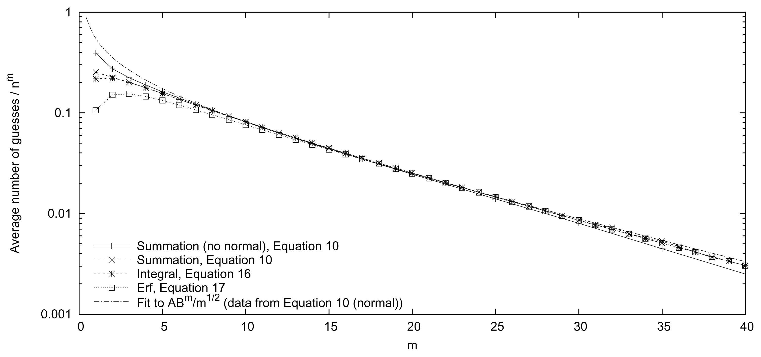
for large values of m [12]. In Figure 3, a comparison of Equations (10) (with both the true and a normal distribution), (16) and (17) is given. The three expressions with a normal distribution give similar values, except for small values of m, and they resemble the expression with the true distribution. The apparent deviation from the true distribution from m = 25 onwards can partly be explained by the logarithmic scale. The absolute deviation decreases, but the relative deviation does not.
By using an asymptotic expansion of the error function [13], it can be shown that the leading term of Equation (17) is:
if
. Thus, the leading term is of the form nm · A · Bm · m−1/2, where A and B are constants for the given probability distribution. The result of fitting the data from Equation (10) (using a normal distribution) to such an expression is displayed in Figure 3. The results will be further discussed in the following section.
4. Results
In this section, two probability distributions will be discussed. First, the distribution given in Figure 1 is investigated in more detail in Section 4.1, and second, the English language is considered in Section 4.2.
4.1. Random Probability Distribution
In Figure 1, the average number of guesses required for correctly guessing a word of size m using an alphabet of size 10 is given using various techniques. First, the exact solution is given (for m < 6). Second, three approximate solutions (as discussed in Section 3) are given (quantification using all probability products could be performed within reasonable time limits only for m < 11). Third, an estimate based on entropy (Equation (7)) is provided. Fourth, lower bounds derived by Massey (Equation (5)) and Arikan (Equation (6)) are included.
As is illustrated in Figure 1, the approximate techniques of quantification (N = 103) and random selection (N = 103, S = 104 and T = 20) may provide accurate estimates of guesswork (with a reasonable amount of storage and CPU time). The third approximate technique (using a normal distribution) (N = 103, S = 104 and T = 20) demonstrates accurate estimates for large values of m (>6) in accordance with the central limit theorem. By using a fitting procedure for values in the range 9 ≤ m ≤ 40, an approximate expression is given by G1/nm ≈ 0.592 · 0.920m · m−1/2 (see Figure 3). By evaluating the leading term of Equation (17) (see Equation (18)), the expression 0.832·0.912m·m−1/2 is obtained.
The exponential entropy expression overestimates guesswork for small values of m (<11) and underestimates it for large values. The lower bound of Massey is closer to the exact value than the lower bound of Arikan. However, both of the lower bounds underestimate the number of guesses by an order of magnitude for m = 20.
Error Estimates
Using the data in Figure 1 and Equation (11), the exact value can be determined to be in the interval [0.999, 1.001] ·
, i.e., the error using quantification (N = 103) is about 0.1%. The additional error of using random selection (N = 103, S = 104 and T = 20) (see Equation (14)) is determined to be between 0.26% and 0.56% (depending on the m value) to a certainty of 99%. The error due to random selection in the normal distribution approximation (N = 103, S = 104 and T = 20) is determined to be between 0.30% and 0.63% (depending on the m value) to a certainty of 99%. Observe that this error does not include the fitness of a normal distribution to the density of the logarithm of probability products.
4.2. English Language
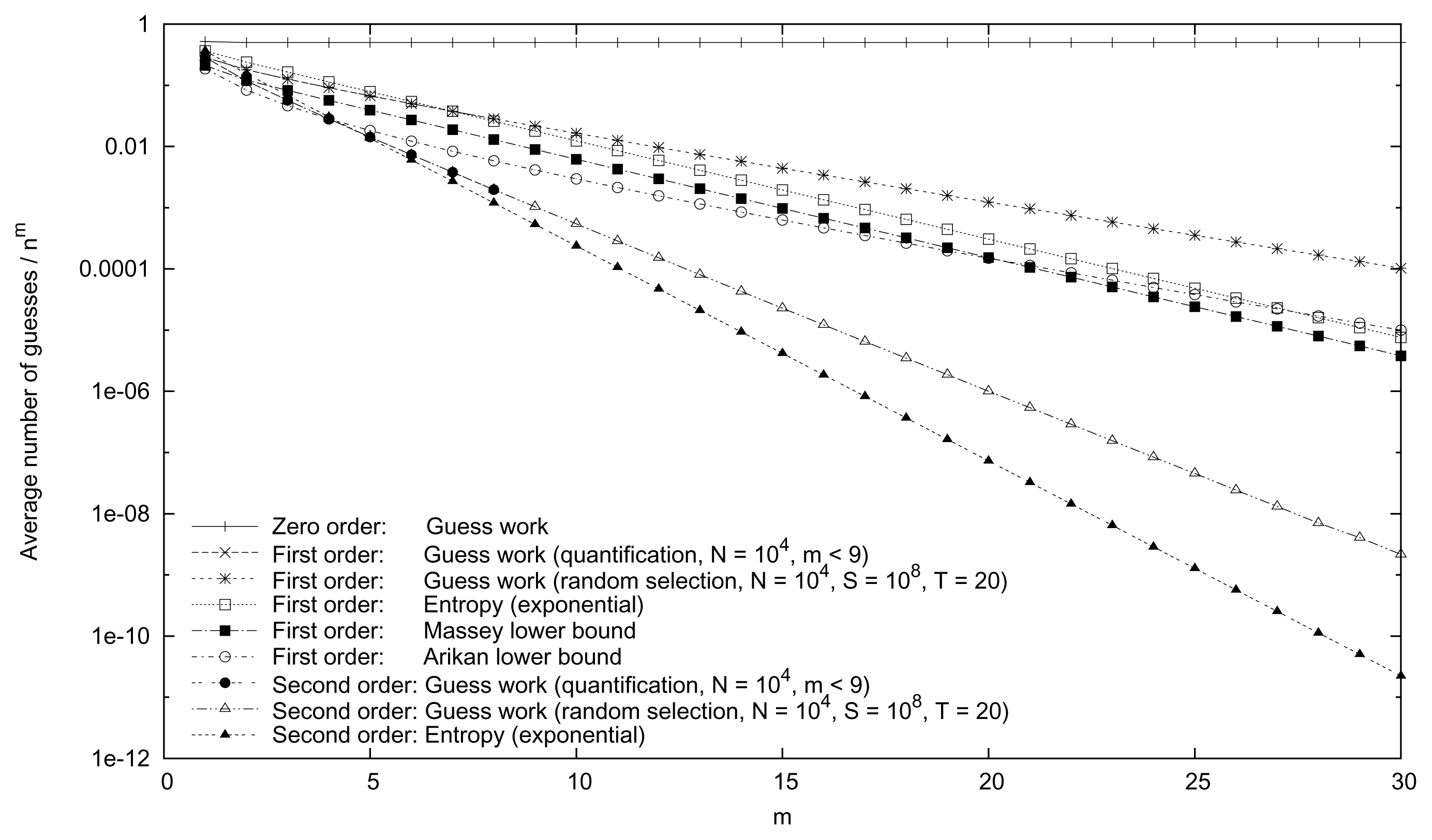
While the probability distribution discussed in the previous section was randomly chosen, the probability distribution considered here originates from the English language [14]. In Appendix, the English bigram frequencies from [14] are repeated. In order to calculate the conditional probability distribution discussed in Section 2.3, each row in the table in Appendix has to be normalized. The probability distribution for each letter in the English alphabet can be obtained by the procedures discussed in Section 2.3. In Figure 4, the average number of guesses required for correctly guessing a word of size m using the English alphabet of size 26 (with the data given in Appendix) is displayed. Guesswork has been numerically evaluated in zero, first and second order. For comparison, estimates based on entropy (Equation (7)) are given in first and second order. In first order, the lower bounds provided by Massey (Equation (5)) and Arikan (Equation (6)) are included.
As is illustrated in Figure 4, all approaches display an exponential behavior (in first and second order) in accordance with Equations (5)–(7) and (17). A normal distribution was not applied, since it is not in agreement with the true distribution. It overestimates guesswork by about an order of magnitude for m = 30. However, it is possible to make a fairly accurate fit of the guesswork data in first and second order to an expression of the form nm · A · Bm · m−1/2, as was discussed in Section 3.3. By using a fitting procedure for the guesswork graphs in Figure 4 for 9 ≤ m ≤ 30, the average number of guesses of words in the English language can be expressed according to the functions in Table 1. The deviation between the true and estimated values (according to Table 1) is less than 10% (except for the smallest m values). For both first and second order, the entropy ansatz underestimates the number of guesses required, for first order by a factor of around 10 and for second order by a factor of around 100 for word lengths of 30. Further, using the extra information provided by a second-order approximation as compared to a first-order approximation reduces the number of guesses by a factor of around 105 for word lengths of 30. The lower bounds of Massey (Equation (5)) and Arikan (Equation (6)) are underestimating the number of guesses by approximately the same amount as the entropy expression for word lengths of 30.
Error Estimates
In first order, the errors introduced by using quantification can be calculated using Equation (11). Using the data in Figure 4, the exact value can be determined to be in the interval [0.9998, 1.0002] ·
, where
is the approximate guess work using quantification for first-order English. In second order, Equation (13) and the data in Figure 4 make it possible to determine that the exact value is in the interval [0.9996, 1.0004] ·
.
Using the same procedure as in Section 4.1, the error introduced when randomly selecting probability products can be estimated. In first order, a 99% confidence interval for the guesswork is given by Equation (14), and by using the data in Figure 4, the error (R1) is determined to be between 0.006% and 0.05% (depending on the m value). This should be added to the error of 0.02% introduced by quantification. In second order, exactly the same procedure can be used, and then, the error is estimated to be in the range 0.006% and 6% (depending on the m value). Again, this error should be added to the error of 0.04% introduced by quantification. The large error introduced by random selection in second order for large m values is due to the fact that the fraction of probability products that are zero is larger for larger m values. By randomly selecting S · m probability products, the number of non-zero probability products is decreasing with an increasing value of m. To increase the accuracy of the guesswork estimate in second order, another m dependence of the number of selected probability products has to be chosen.
5. Conclusions
In the paper, it has been demonstrated that it is possible to estimate the average number of guesses (guesswork) of a word with a given length numerically with reasonable accuracy (to a couple of percent) for large alphabet sizes (≈ 100) and word lengths (≈ 100) within minutes. Thus, a numerical estimate of guesswork constitutes an alternative to, e.g., various entropy expressions.
For many probability distributions, the density of the logarithm of probability products is close to a normal distribution. For those cases, it is possible to derive an analytical expression for guesswork showing the functional dependence of the word length. The proportion of guesses needed on average compared to the total number decreases almost exponentially with the word length. The leading term in an asymptotic expansion of guesswork has the form nm · A · Bm · m−1/2, where A and B are constants (however, different for different probability distributions), n is the size of the alphabet and m is the word length. Such an expression can be determined for medium-sized values of m, using some fitting procedure, and used with fairly good accuracy for large values of m.
In the paper, the English language has been investigated. The average number of guesses has been calculated numerically in both first and second order giving a reduction of the number of guesses by a factor 105 for word lengths of 30 when the extra information provided by second order is included. A normal distribution of the logarithm of probability products was not applied, since it is not in agreement with the true distribution. It overestimates guesswork by about an order of magnitude for word lengths of 30. Still, it is possible to find accurate expressions for guesswork (0.481 · 0.801m · m−1/2 in first order and 0.632 · 0.554m · m−1/2 in second order) in agreement with the true values (the deviation is less than 10% for word lengths of 30).
A comparison between guesswork and entropy expressions has been performed showing that the entropy ansatz underestimates the number of guesses required, for first order by a factor of around 10 and for second order by a factor of around 100 for English words of length 30. Lower bounds of guesswork by Massey and Arikan have also been investigated. They are underestimating the number of guesses by approximately the same amount as the entropy expression for word lengths of 30.
Acknowledgments
The author would like to thank Ångpanneföreningens Forskningsstiftelse for a traveling scholarship. The author would also like to thank the valuable remarks and comments received in connection with the conferences CiE2012 and UCNC2012 and by the reviewers of this manuscript.
Appendix: English Bigram Frequencies
The information in the matrix below is used for creating matrix P used in Section 2.3 [14]. After normalization of each row, matrix P is obtained.

| A | B | C | D | E | F | G | H | I | J | K | L | M | N | O | P | Q | R | S | T | U | V | W | X | Y | Z | |
|---|---|---|---|---|---|---|---|---|---|---|---|---|---|---|---|---|---|---|---|---|---|---|---|---|---|---|
| A | 1 | 32 | 39 | 15 | 0 | 10 | 18 | 0 | 16 | 0 | 10 | 77 | 18 | 172 | 2 | 31 | 1 | 101 | 67 | 124 | 12 | 24 | 7 | 0 | 27 | 1 |
| B | 8 | 0 | 0 | 0 | 58 | 0 | 0 | 0 | 6 | 2 | 0 | 21 | 1 | 0 | 11 | 0 | 0 | 6 | 5 | 0 | 25 | 0 | 0 | 0 | 19 | 0 |
| C | 44 | 0 | 12 | 0 | 55 | 1 | 0 | 46 | 15 | 0 | 8 | 16 | 0 | 0 | 59 | 1 | 0 | 7 | 1 | 38 | 16 | 0 | 1 | 0 | 0 | 0 |
| D | 45 | 18 | 4 | 10 | 39 | 12 | 2 | 3 | 57 | 1 | 0 | 7 | 9 | 5 | 37 | 7 | 1 | 10 | 32 | 39 | 8 | 4 | 9 | 0 | 6 | 0 |
| E | 131 | 11 | 64 | 107 | 39 | 23 | 20 | 15 | 40 | 1 | 2 | 46 | 43 | 120 | 46 | 32 | 14 | 154 | 145 | 80 | 7 | 16 | 41 | 17 | 17 | 0 |
| F | 21 | 2 | 9 | 1 | 25 | 14 | 1 | 6 | 21 | 1 | 0 | 10 | 3 | 2 | 38 | 3 | 0 | 4 | 8 | 42 | 11 | 1 | 4 | 0 | 1 | 0 |
| G | 11 | 2 | 1 | 1 | 32 | 3 | 1 | 16 | 10 | 0 | 0 | 4 | 1 | 3 | 23 | 1 | 0 | 21 | 7 | 13 | 8 | 0 | 2 | 0 | 1 | 0 |
| H | 84 | 1 | 2 | 1 | 251 | 2 | 0 | 5 | 72 | 0 | 0 | 3 | 1 | 2 | 46 | 1 | 0 | 8 | 3 | 22 | 2 | 0 | 7 | 0 | 1 | 0 |
| I | 18 | 7 | 55 | 16 | 37 | 27 | 10 | 0 | 0 | 0 | 8 | 39 | 32 | 169 | 63 | 3 | 0 | 21 | 106 | 88 | 0 | 14 | 1 | 1 | 0 | 4 |
| J | 0 | 0 | 0 | 0 | 2 | 0 | 0 | 0 | 0 | 0 | 0 | 0 | 0 | 0 | 4 | 0 | 0 | 0 | 0 | 0 | 4 | 0 | 0 | 0 | 0 | 0 |
| K | 0 | 0 | 0 | 0 | 28 | 0 | 0 | 0 | 8 | 0 | 0 | 0 | 0 | 3 | 3 | 0 | 0 | 0 | 2 | 1 | 0 | 0 | 3 | 0 | 3 | 0 |
| L | 34 | 7 | 8 | 28 | 72 | 5 | 1 | 0 | 57 | 1 | 3 | 55 | 4 | 1 | 28 | 2 | 2 | 2 | 12 | 19 | 8 | 2 | 5 | 0 | 47 | 0 |
| M | 56 | 9 | 1 | 2 | 48 | 0 | 0 | 1 | 26 | 0 | 0 | 0 | 5 | 3 | 28 | 16 | 0 | 0 | 6 | 6 | 13 | 0 | 2 | 0 | 3 | 0 |
| N | 54 | 7 | 31 | 118 | 64 | 8 | 75 | 9 | 37 | 3 | 3 | 10 | 7 | 9 | 65 | 7 | 0 | 5 | 51 | 110 | 12 | 4 | 15 | 1 | 14 | 0 |
| O | 9 | 18 | 18 | 16 | 3 | 94 | 3 | 3 | 13 | 0 | 5 | 17 | 44 | 145 | 23 | 29 | 0 | 113 | 37 | 53 | 96 | 13 | 36 | 0 | 4 | 2 |
| P | 21 | 1 | 0 | 0 | 40 | 0 | 0 | 7 | 8 | 0 | 0 | 29 | 0 | 0 | 28 | 26 | 0 | 42 | 3 | 14 | 7 | 0 | 1 | 0 | 2 | 0 |
| Q | 0 | 0 | 0 | 0 | 0 | 0 | 0 | 0 | 0 | 0 | 0 | 0 | 0 | 0 | 0 | 0 | 0 | 0 | 0 | 0 | 20 | 0 | 0 | 0 | 0 | 0 |
| R | 57 | 4 | 14 | 16 | 148 | 6 | 6 | 3 | 77 | 1 | 11 | 12 | 15 | 12 | 54 | 8 | 0 | 18 | 39 | 63 | 6 | 5 | 10 | 0 | 17 | 0 |
| S | 75 | 13 | 21 | 6 | 84 | 13 | 6 | 30 | 42 | 0 | 2 | 6 | 14 | 19 | 71 | 24 | 2 | 6 | 41 | 121 | 30 | 2 | 27 | 0 | 4 | 0 |
| T | 56 | 14 | 6 | 9 | 94 | 5 | 1 | 315 | 128 | 0 | 0 | 12 | 14 | 8 | 111 | 8 | 0 | 30 | 32 | 53 | 22 | 4 | 16 | 0 | 21 | 0 |
| U | 18 | 5 | 17 | 11 | 11 | 1 | 12 | 2 | 5 | 0 | 0 | 28 | 9 | 33 | 2 | 17 | 0 | 49 | 42 | 45 | 0 | 0 | 0 | 1 | 1 | 1 |
| V | 15 | 0 | 0 | 0 | 53 | 0 | 0 | 0 | 19 | 0 | 0 | 0 | 0 | 0 | 6 | 0 | 0 | 0 | 0 | 0 | 0 | 0 | 0 | 0 | 0 | 0 |
| W | 32 | 0 | 3 | 4 | 30 | 1 | 0 | 48 | 37 | 0 | 0 | 4 | 1 | 10 | 17 | 2 | 0 | 1 | 3 | 6 | 1 | 1 | 2 | 0 | 0 | 0 |
| X | 3 | 0 | 5 | 0 | 1 | 0 | 0 | 0 | 4 | 0 | 0 | 0 | 0 | 0 | 1 | 4 | 0 | 0 | 0 | 1 | 1 | 0 | 0 | 0 | 0 | 0 |
| Y | 11 | 11 | 10 | 4 | 12 | 3 | 5 | 5 | 18 | 0 | 0 | 6 | 4 | 3 | 28 | 7 | 0 | 5 | 17 | 21 | 1 | 3 | 14 | 0 | 0 | 0 |
| Z | 0 | 0 | 0 | 0 | 5 | 0 | 0 | 0 | 2 | 0 | 0 | 1 | 0 | 0 | 0 | 0 | 0 | 0 | 0 | 0 | 0 | 0 | 0 | 0 | 0 | 1 |
Conflicts of Interest
The authors declare no conflict of interest.
References and Notes
- Christiansen, M.M.; Duffy, K.R. Guesswork, large deviations, and Shannon entropy. IEEE Trans. Inf. Theory 2013, 59, 796–802. [Google Scholar]
- Dürmuth, M.; Chaabane, A.; Perito, D.; Castelluccia, C. When privacy meets security: Leveraging personal infomation for password cracking 2013. arXiv:1304.6584v1.
- Pliam, J.O. The disparity between work and entropy in cryptology; Available online: http://eprint.iacr.org/1998/024 accessed on 5 October 2014.
- Lundin, R.; Lindskog, S.; Brunström, A.; Fischer-Hübner, S. Using guesswork as a measure for confidentiality of selectivly encrypted messages. In Advances in Information Security; Gollmann, D., Massacci, F., Yautsiukhin, A., Eds.; Springer: New York, NY, USA, 2006; Volume 23, pp. 173–184. [Google Scholar]
- Arikan, E. An inequality on guessing and its application to sequential decoding. IEEE Trans. Inf. Theory 1996, 42, 99–105. [Google Scholar]
- Massey, J.L. Guessing and entropy. Proceedings of the 1994 IEEE International Symposium on Information Theory, Trondheim, Norway, 27 June–1 July 1994; p. 204.
- Andersson, K. Numerical evaluation of the average number of successive guesses. In Unconventional Computation and Natural Computation; Proceedings of 11th International Conference on Unconventional Computation and Natural Computation (UCNC 2012), Orléans, France, 3–7 September, 2012, Lecture Notes in Computer Science; Volume 7445, Durand-Lose, J., Jonoska, N., Eds.; Springer: Berlin/Heidelberg, Germany, 2012; p. 234. [Google Scholar]
- Shannon, C.E. A mathmatical theory of communication. Bell Syst. Tech. J 1948, 27. [Google Scholar]
- Malone, D.; Sullivan, W. Guesswork is not a substitute for entropy. Proceedings of the Information Technology and Telecommunications Conference, Cork, Ireland, 26–27 October 2005.
- Cover, T.M.; Thomas, J.A. Elements of Information Theory, 2nd ed; Wiley: Hoboken, NJ, USA, 2006. [Google Scholar]
- Box, G.E.P.; Hunter, J.S.; Hunter, W.G. Statistics for Experimenters: Design, Innovation and Discovery, 2nd ed; Wiley: Hoboken, NJ, USA, 2005. [Google Scholar]
- Erf. Available online: http://mathworld.wolfram.com/Erf.html accessed on 5 October 2014. from this source the integral has been used.
- for large x
- Nicholl, J. Available online: http://jnicholl.org/Cryptanalysis/Data/DigramFrequencies.php accessed on 5 October 2014.
Figure 1.
The quotient of the average and the maximum number of guesses of words of size m for the randomly chosen probability distribution given to the right (n = 10).
Figure 1.
The quotient of the average and the maximum number of guesses of words of size m for the randomly chosen probability distribution given to the right (n = 10).

Figure 2.
The density of the logarithm of products of probabilities for a randomized probability distribution (given by Figure 1) for n = 10 and N = 10. Random selection with S = 108 is used for m = 20. Base e is adopted. The average value is μ1m, and the standard deviation
, where the values μ1 = 0.824535 and σ1 = 0.678331 have been obtained by a least squares fit of the μ and σ from the normal distribution fitted densities for m = 6, 8, 10, . . ., 50.

Figure 3.
The guesswork for the randomized probability distribution given in Figure 1 (n = 10). For one summation, the true density of the logarithm of probabilities is used (N = 10, S = 10, 000 and T = 20), and otherwise, a normal distribution is used (with the data given in Figure 2 and N = 10 for Equation (10)).

Figure 4.
The quotient of the average and the maximum number of guesses of words of size m in the English language (n = 26).
Figure 4.
The quotient of the average and the maximum number of guesses of words of size m in the English language (n = 26).

Table 1.
The average number of guesses of words of length m in English divided by the maximum number.
| Order | Expression |
|---|---|
| 0 | 1/2 |
| 1 | 0.481 · 0.801m · m−1/2 |
| 2 | 0.632 · 0.554m · m−1/2 |
© 2014 by the authors; licensee MDPI, Basel, Switzerland This article is an open access article distributed under the terms and conditions of the Creative Commons Attribution license (http://creativecommons.org/licenses/by/3.0/).
Share and Cite
MDPI and ACS Style
Andersson, K. Exact Probability Distribution versus Entropy. Entropy 2014, 16, 5198-5210. https://doi.org/10.3390/e16105198
AMA Style
Andersson K. Exact Probability Distribution versus Entropy. Entropy. 2014; 16(10):5198-5210. https://doi.org/10.3390/e16105198
Chicago/Turabian StyleAndersson, Kerstin. 2014. "Exact Probability Distribution versus Entropy" Entropy 16, no. 10: 5198-5210. https://doi.org/10.3390/e16105198