Fluctuations, Entropic Quantifiers and Classical-Quantum Transition

Abstract
: We show that a special entropic quantifier, called the statistical complexity, becomes maximal at the transition between super-Poisson and sub-Poisson regimes. This acquires important connotations given the fact that these regimes are usually associated with, respectively, classical and quantum processes.1. Introduction
This work deals with aspects of the transition between classical and quantum regimes, a subject of much current interest. This is done in terms of an entropic quantifier called the statistical complexity and the methodology employed is the examination of energy fluctuations, that are shown to play a pivotal role in the concomitant considerations. Indeed, our main quantifier (a complexity measure) becomes expressed solely in fluctuations’ terms. We begin by introducing below the main ingredients of our developments.
1.1. Statistical Complexity
A statistical complexity measure (SCM) is a functional that characterizes any given probability distribution P. It quantifies not only randomness but also the presence of correlational structures, being represented by an appropriate functional C [P]. Among a panoply of references, see for instance, [1–4].
It has been acknowledged for a long time that simply accounting for information (as the Shannon or Fisher information measures do), does not fully grasp the notion of complexity, since a perfect chaos maximizes information but it is actually not much more complex than perfect order. As Crutchfield noted in 1994, Physics does have the tools for detecting and measuring complete order—equilibria and fixed point or periodic behavior—and ideal randomness—via temperature and thermodynamic entropy or, in dynamical contexts, via the Shannon entropy rate and Kolmogorov complexity. What is still needed, though, is a definition of structure and way to detect and to measure it [5]. Seth Lloyd counted as many as 40 ways to define complexity, none of them being completely satisfactory. A major breakthrough came from the definition proposed by Lopez-Ruiz, Mancini and Calbet (LMC) [1]. Although not exempt from minor problems [6], LMC’s complexity clearly separated and quantified the contributions of entropy and structure. The main feature of a statistical complexity measures is that it should be minimal both for complete randomness and for perfect order.
1.2. Classical Limit of Quantum Mechanics
The classical limit of quantum mechanics is a subject that continues attracting much attention, and can be regarded as one of the multiple frontiers of physics’ research. Certainly, it is the source of much exciting discussion (see, for instance, [7,8] and references therein).
One interesting case is that of a semiclassical model for which one clearly distinguishes [9,10] three zones, namely,
One deals here with a special bipartite system that represents the zero-th mode contribution of a strong external field to the production of charged meson pairs [11–13]. It is well known that, for this model, the classic to quantum route traverses high complexity intermediate regions (of the appropriate phase space in which “the action” takes place) where chaos reigns, interrupted often by quasi-periodic windows (See Kowalski et al. [9,10].)
1.3. Motivation and Goals
The motivation of the present endeavor is the fact that plenty of evidence indicates that the statistical complexity is maximal in the transition region between classical and quantum regimes [14,15]. Here we reconfirm such results for a much simpler Hamiltonian than the one of [14,15], that of the Harmonic Oscillator (HO). This is a really important system and HO insights usually have a wide impact. Thus, the HO constitutes much more than a mere simple example. Nowadays, it is of particular interest for the dynamics of bosonic or fermionic atoms contained in magnetic traps [16–18] as well as for any system that exhibits an equidistant level spacing in the vicinity of the ground state, like nuclei or Luttinger liquids. This article is organized as follows:
We begin our considerations in Section 2 by computing the Fano factor for a general Gaussian distribution of width 1/δ and linking δ to several phase space’s information-quantifiers.
In Section 3 we apply the above considerations to physical examples.
Finally, some conclusions are drawn in Section 4.
2. Entropic Quantifiers For Gaussian Distributions in Phase Space
As befits a classical-quantum transition’s description, we are going to employ the Wigner phase space representation of quantum mechanics, as explained in detail, for example, in [19]. The HO Hamiltonian reads in this case
where α refers to the standard coherent states |α〉 of the harmonic oscillator. These are eigenstates of the annihilation operator â, with complex eigenvalues α, satisfying â|α〉 = α|α〉. They are denoted in Dirac notation as [20]
where |n〉 are a complete orthonormal set of eigenstates of the HO quantum Hamiltonian Ĥ = ħω(â†â+1/2), whose spectrum is En = (n + 1/2)ħω, n = 0, 1, . . .
A coherent state |α〉 is a specific kind of quantum state, the one that most resembles a classical state. The states |α〉 are normalized, i.e., 〈α|α〉 = 1, and they provide us with a resolution of the identity operator
which is a completeness relation for the coherent states [20], with d2α/π = dxdp/2πħ. Note we have added 1/π for normalization’s sake.
In order to visualize the coherent states one introduces a pair of Hermitian operators x̂ and p̂ to represent, respectively, the coordinate of the oscillator and its momentum [20]. These operators satisfy the canonical commutation relations [x̂, p̂] = iħ. Then, one has
2.1. Energy Fluctuations
Let us now introduce a gaussian distribution of variance 1/δ, that in phase space acquires the form
where f(α) is normalized according to
Many important physical situations are characterized by this type of distributions, as discussed below. Now, not any δ-value will yield a quantum Gaussian distribution. This is so because, if ρ̂ is the density operator, then we have the constraint Tr ρ̂2 ≤ Tr ρ̂. This translates into
and one immediately finds that, for this to be true one needs
Accordingly, the distribution f’s width (1/δ) cannot be too small without entering into conflict with the uncertainty principle, here referred to location in phase space. The energy fluctuations are given by the root mean square deviation of the Hamiltonian H0 from its average 〈H0〉, so that
where the statistical expectation value of |α|s in phase space are computed as follows
with s = 2, 4 and f(α) is considered a statistical weight function. Thus, it is clear that
The coefficient of dispersion of the probability distribution f(α) is defined as
being usually known as the Fano factor [21]. Consider x = |α|2. In this case we have
and the Fano factor becomes
which is, for a Gaussian distribution, a universal relation linking the Fano factor to the distribution’s width.
2.2. Entropic Quantifiers
A very important information-quantifier is the so called Fisher’s information measure (FIM) [22,23]. Its phase space representation is [24]
For some applications and details of this measure see, amongst many possibilities [22,23,25]. From Equation (7) and integrating over phase space, the Fisher measure acquires the form
and we appreciate the fact that I is inversely proportional to the width of the distribution, ranging within the interval [0, 2].
The statistical complexity C à la LMC is a suitable product of two quantifiers, such that C becomes minimal at the extreme situations of perfect order or total randomness. We will take one of the quantifiers to be Fisher’s measure and the other an entropic form, since it is well known that the two behave in opposite manner [22]. A possibility is to consider the Manfredi-Feix entropy [26], derived from the phase space Tsallis (q = 2) entropy [27]. In quantum information this form is referred to as the linear entropy [28]. It reads
Accordingly, we have
and the ensuing complexity becomes
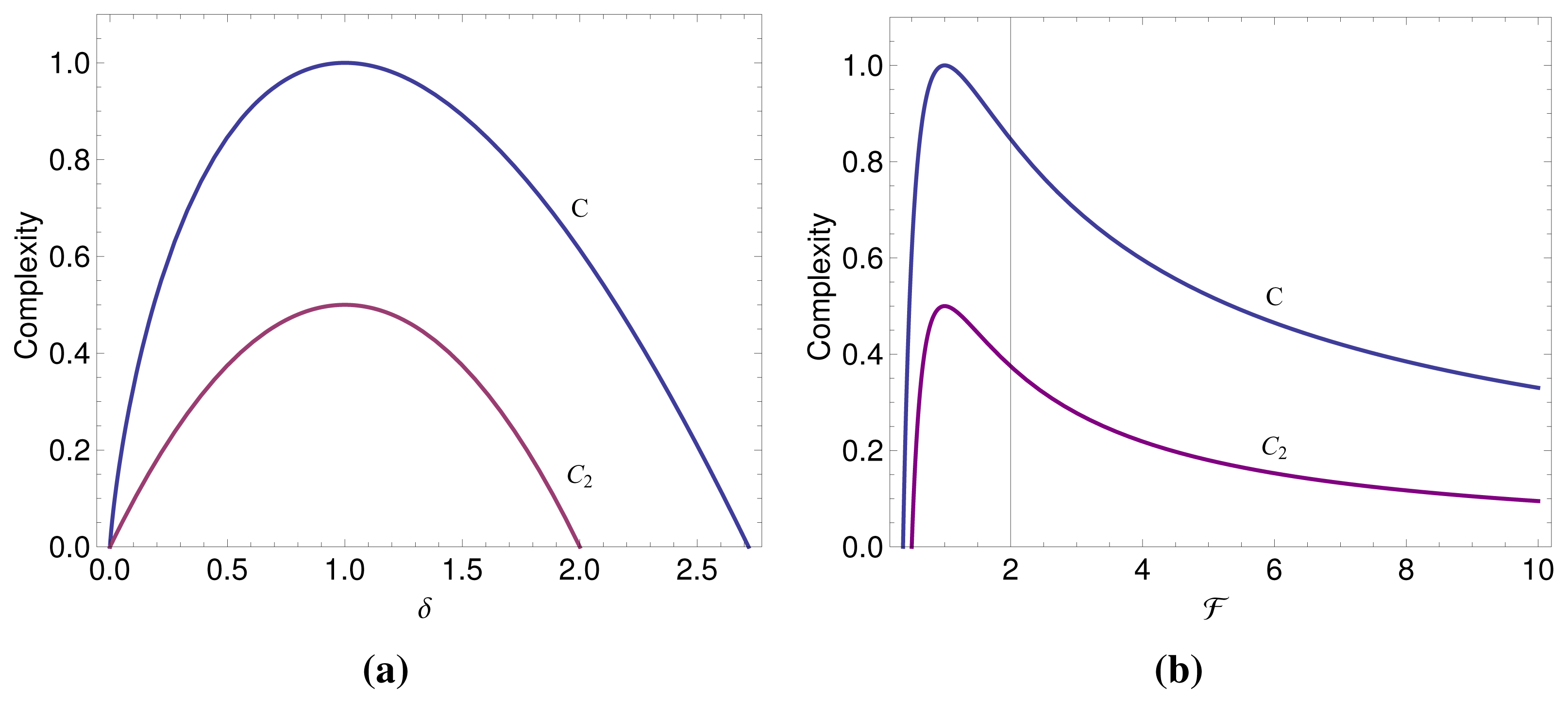
vanishing both for δ = 0 and for δ = 2, the extreme values of the δ-range. It is easy to see that the derivative of C2 with respect to δ vanishes at δ = 1. Consideration of the second derivative allows one to ascertain that we have a maximum there. The physical meaning of this maximum will be ascertained below, in discussing sub- and super-Poissonian regimes. The change between them takes place at δ = 1.
Alternatively, the logarithmic Shannon’s information measure (entropy) is expressed in phase space as
that reduces to
One possible form for the statistical complexity, minimal for perfect order or total randomness, acquires the appearance
with
It is easy to verify that C vanishes both for δ = 0 and for δ = e. This last value lies outside our physical zone, and thus cannot be considered. In any case, within the physical range C is, on the right-hand side of (1/δ) = 1, relatively minimal at δ = 2. One easily ascertains that the complexity-maximum is to be found, again, at δ = 1, for our two entropic quantifiers. In Figure 1 the statistical complexity is plotted in terms of the inverse variance δ. We insist on the fact that our two complexities are maximal at δ = 1. Also, from Equations (16) and (18) we get
and, therefore, we can rewrite the complexities C2 and C in terms of the Fano factor as follows
and
The complexity-maximum is obtained from dC2/ = 0, and dC/d = 0, that implies = 1 entailing C = 1, and C2 = 1/2. One appreciates the fact that the statistical complexity can be expressed solely in fluctuation terms.
The expressions of the complexities C and C2 are plotted in Figure 1.
2.3. Interpreting Relative Energy Fluctuations
If one constructs a Poisson distribution in the variable |α|2, one immediately realizes that the associated Fano factor becomes unity [29,30]. Thus, for a Poisson process the variance in the count equals the mean count. For instance, in optics one has that
for < 1, emitted light is referred to as sub-Poissonian since it has photo-count noise smaller than that of coherent (ideal laser) light with the same intensity ( = 1), and speaks of non-classical light, whereas
for > 1, the light is called super-Poissonian, exhibiting photo-count noise higher than the coherent-light noise.
Accordingly, the Fano factor may be regarded as a non-classicality indicator, with < 1 only in a quantum regime. One speaks of nonclassical light, i.e., light that cannot be described using classical electromagnetism; its characteristics being described by the quantized electromagnetic field and quantum mechanics [31]. Nonclassical light has nonclassical noise properties called quantum noise [32].
Thus, we realize here that the statistical complexity, as stated in the previous Section, attains a maximum at δ = 1, that is, just at the frontier between the classical super- and quantum sub-Poissonian regions. Such maximum becomes then a signature of the classical-quantum transition, the main result of the present work. Note that the result is robust in the sense that it is valid for two different entropic quantifiers. Importantly enough, the result is analytic and thus not open to numerical discussions.
3. Physical Examples of Gaussian Distributions
3.1. Thermal States
We focus attention now on the field emitted by a source in thermal equilibrium at temperature T (thermal state) [29,30] and have
where kB is the Boltzmann constant. Then, for the HO quantum Hamiltonian Ĥ one obtains [33]
with β = 1/kBT. Three important Gaussian distributions can be used in this context, as discussed below.
3.2. P-States
The most general density operator is just a superposition of the projection operators |α〉〈α|, known as the P-representation (normally ordered field operators), whose form is [29,33]
where the function P(α, α*) plays a role analogous to a probability density for the distribution of values of α over the complex plane. In general, P(α, α*) is a generalized function (Schwartz distribution). We speak of the P-representation or of the coherent state representation [33]. P(α, α*) forms the connection between the classical and quantum coherence theory. P can be regarded as well as a quasi probability distribution function because it can have negative values and strong singularities, specially when the density operator corresponds to a nonclassical state with sub-Poisson photon statistics (see [29] and references therein).
When the P-function tends to vary little over large ranges of the parameter α, the nonorthogonality of the coherent states will make little difference, and P(α, α*) (to be abbreviated here from as P(α)) can be interpreted as a probability distribution [29]. The expectation value of an observable  is given by [29]
The central quantity of our treatment, has a simple form that, of course, can be written in the fashion [20]
In view of these arguments, one has for the variance of |α|2
with the statistical averages
where s = 2, 4. One has [33]
with
where n̂ = a†â is the photon number operator.
3.3. Husimi Functions
The Husimi [34], or Q-representation, is associated with the evaluation of anti normally ordered creation and destruction operators (as compared with the P-representation above, connected to normally ordered correlation functions [29]). For the density matrix ρ̂ of Equation (29) one can always write [24]
where Z stands for the canonical partition function In this situation we have at our disposal the useful analytic expressions given for HO system, for instance, in [24,35] and one ends up with a Gaussian distribution [35]
3.4. Wigner Distributions
Finally, obligatory reference must be made now to the celebrated Wigner quasi-probability distribution DW(x, p) (also called the Wigner function), a special type of quasi-probability distribution that was introduced by Eugene Wigner in 1932 [36] to study quantum corrections to classical statistical mechanics. In trying to approximate it in some fashion one is prone to fall into the semiclassical domain. Wigner’s goal was to supplant the wave-function that appears in Schrödinger’s equation with a probability distribution DW in phase space. This DW should function as a generating function for all spatial autocorrelation functions of a given quantum-mechanical wave-function ψ(x). For the Hamiltonian H0, DW is a Gaussian too [37].
3.5. Inverse Variances δ For Our Gaussian States
We collect below the inverse variances and the associated Fano factors for our three instances of quantum Gaussian functions, namely, P, Q, and Wigner’s [33].
- (1)
P-functions: δ = 1/〈n̂〉 = (1 – e−βħω)/e−βħω ⇒ P = e−βħω/(1 – e−βħω),
- (2)
Husimi functions Q: δ = 1– e−βħω ⇒ H = 1/(1 – e−βħω),
- (3)
Wigner functions W: δ = 2 tanh(βħω/2) ⇒ W = 1/2 tanh(βħω/2).
The Einstein temperatures are defined as TE = ħω/kB and are indicators of the rigidity of Einstein’s lattice. The critical ratios θ = kBT/ħω at which the Fano factor become unity, and there is a change of regime from sub-Poisonnian (quantum regime) to super Possonian (classical), are:
where θH, θP, θW are the critical ratios for the Husimi function, P-function, and Wigner function respectively.
In our two entropic cases we have, of course,
and the entropies become
- (1)
SH = 1– ln(1 – e−βħω),
- (2)
SW = 1– ln[2 tanh(βħω/2)],
- (3)
SP = 1– ln(eβħω – 1),
- (4)
S2H = 1– (1 – e−βħω)/2,
- (5)
S2W = 1– tanh(βħω/2),
- (6)
S2P = 1– (eβħω – 1)/2.
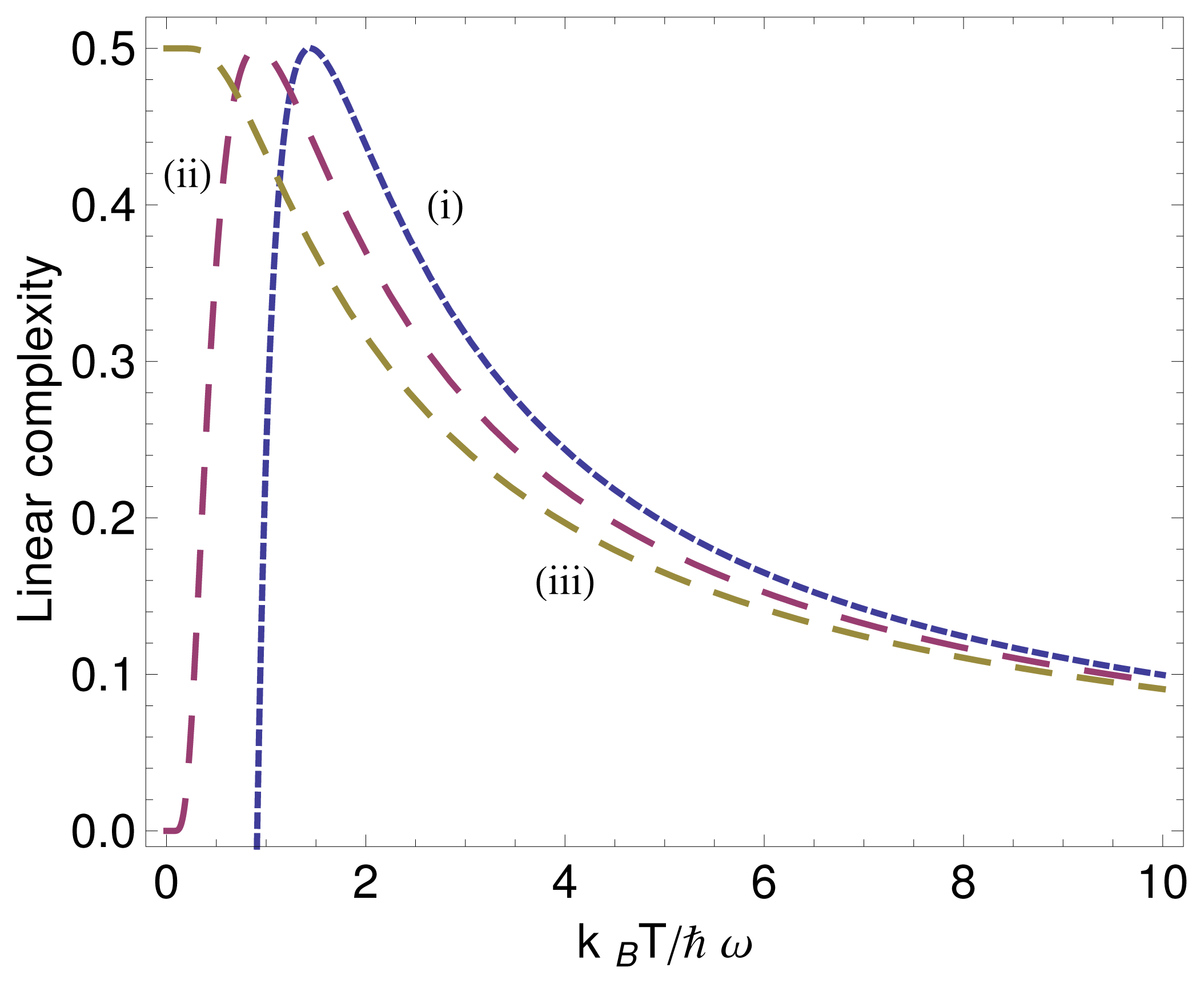
The corresponding linear complexities are:
- (1)
C2P = S2P IP,
- (2)
C2W = S2W IW,
- (3)
C2H = S2H IH.
We see in Figure 2 the behavior of the linear complexity as a function of temperature T for the three cases mentioned above.
4. Conclusions
This paper tried to illustrate on the usefulness of the statistical complexity quantifier as a phase-transition indicator, as has been hinted in several precedent works dealing with rather complex environments, like that of the Cooper et al. model [11–13], the brain’s electrical activity [38], or collective motion [39].
The complicated structure of the quantum-classical phase transitions discussed by Kowalski et al. [12,13], simplifies enormously for the harmonic oscillator. Thus, here we see the complexity phase-transition detecting effect in the simplest possible fashion (the HO), and the ensuing treatment is of an analytical character, referring to the transition between super-Poisson and sub-Poisson regimes.
Such transition can be assimilated to a classical-quantal one [29], which makes our present results to agree with those derived for the entirely different scenario of Cooper model in [14,15].
We employed three important types of physical Gaussian states, namely, P-distributions, Husimi functions and Wigner, and we have had the opportunity of discussing things in a temperature dependent context. We have used two different forms for the SC and obtained the same result: the transition takes place at the Gaussian’s inverse-width δ = 1.
Acknowledgment
Flavia Pennini would like to thank partial financial support by FONDECYT, grant 1110827. This work was also partially supported by the project PIP1177 of CONICET (Argentina), and the projects FIS2008-00781/FIS (MICINN)-FEDER (EU) (Spain, EU).
Conflict of Interests
The authors declare no conflict of interest.
- Author ContributionFlavia Pennini and Angelo Plastino designed research, performed research and wrote the paper. Both authors read and approved the final manuscript.
References
- López-Ruiz, R.; Mancini, H.L.; Calbet, X. A statistical measure of complexity. Phys. Lett. A 1995, 209, 321–326. [Google Scholar]
- Feldman, D.P.; Crutchfield, J.P. Measures of statistical complexity: Why? Phys. Lett. A 1998, 238, 244–252. [Google Scholar]
- Lamberti, P.W.; Martín, M.T.; Plastino, A.; Rosso, O.A. Intensive entropic non-triviality measure. Physica A 2004, 334, 119–131. [Google Scholar]
- Martín, M.T.; Plastino, A.; Rosso, O.A. Generalized statistical complexity measures: Geometrical and analytical properties. Physica A 2006, 369, 439–462. [Google Scholar]
- Crutchfield, J.P. The calculi of emergence: Computation, dynamics and induction. Physica D 1994, 75, 11–54. [Google Scholar]
- Anteneodo, C.; Plastino, A.R. Some features of the López Ruiz-Mancini-Calbet (LMC) statistical measure of complexity. Phys. Lett. A 1996, 223, 348–354. [Google Scholar]
- Halliwell, J.J.; Yearsley, J.M. Arrival times, complex potentials, and decoherent histories. Phys. Rev. A 2009, 79, 062101. [Google Scholar]
- Everitt, M.J.; Munro, W.J.; Spiller, T.P. Quantum-classical crossover of a field mode. Phys. Rev. A 2009, 79, 032328. [Google Scholar]
- Kowalski, A.M.; Martín, M.T.; Plastino, A.; Proto, A.N. Classical limit and chaotic regime in a semi-quantum Hamiltonian. Int. J. Bifurc. Chaos 2003, 13, 2315–2325. [Google Scholar]
- Kowalski, A.M.; Martín, M.T.; Plastino, A.; Proto, A.N.; Rosso, O.A. Wavelet statistical complexity analysis of classical limit. Phys. Lett. A 2003, 311, 180–191. [Google Scholar]
- Cooper, F.; Dawson, J.; Habib, S.; Ryne, R.D. Chaos in time-dependent variational approximations to quantum dynamics. Phys. Rev. E 1998, 57, 1489–1498. [Google Scholar]
- Kowalski, A.M.; Martín, M.T.; Nuñez, J.; Plastino, A.; Proto, A.N. Quantitative indicator for semiquantum chaos. Phys. Rev. A 1998, 58, 2596–2599. [Google Scholar]
- Kowalski, A.M.; Plastino, A.; Proto, A.N. Classical limits. Phys. Lett. A 2002, 297, 162–172. [Google Scholar]
- Kowalski, A.M.; Martín, M.T.; Plastino, A.; Rosso, O.A. Chaos and complexity in the classical-quantum transition. Int. J. Appl. Math. Stat 2012, 26, 67–80. [Google Scholar]
- Kowalski, A.; Plastino, A. The Tsallis-complexity of a semiclassical time-evolution. Physica A 2012, 391, 5375–5383. [Google Scholar]
- Anderson, M.H.; Ensher, J.R.; Matthews, M.R.; Wieman, C.E.; Cornell, E.A. Observation of Bose-Einstein condensation in a dilute atomic vapor. Science 1995, 269, 198–201. [Google Scholar]
- Davis, K.B.; Mewes, M.O.; Andrews, M.R.; van Druten, N.J.; Durfee, D.S.; Kurn, D.M.; Ketterle, W. Bose-Einstein condensation in a gas of sodium atoms. Phys. Rev. Lett 1995, 75, 3969–3973. [Google Scholar]
- Bradley, C.C.; Sackett, C.A.; Hulet, R.G. Bose-Einstein condensation of lithium: Observation of limited condensate number. Phys. Rev. Lett 1997, 78, 985–989. [Google Scholar]
- Zachos, C.K.; Fairlie, D.; Curtright, T. Quantum Mechanics in Phase Space; World Scientific: Singapore, Singapore, 2005. [Google Scholar]
- Glauber, R.J. Coherent and incoherent states of the radiation field. Phys. Rev 1963, 131, 2766–2788. [Google Scholar]
- Fano, U. Ionization yield of radiations. II. The fluctuations of the number of ions. Phys. Rev 1947, 72, 26–29. [Google Scholar]
- Frieden, B.R. Science from Fisher Information, 2nd ed; Cambridge University Press: Cambridge, UK, 2008. [Google Scholar]
- Olivares, F.; Pennini, F.; Plastino, A. Note on semiclassical uncertainty relations. Braz. J. Phys 2009, 39, 503–506. [Google Scholar]
- Pennini, F.; Plastino, A. Heisenberg-Fisher thermal uncertainty measure. Phys. Rev. E 2004, 69, 057101. [Google Scholar]
- Pennini, F.; Plastino, A.; Ferri, G.L. Temperature effects, Frieden-Hawkins’ order-measure, and Wehrl entropy. Entropy 2012, 14, 2081–2099. [Google Scholar]
- Manfredi, G.; Feix, M.R. Entropy and Wigner functions. Phys. Rev. E 2000, 62, 4665–4674. [Google Scholar]
- Tsallis, C. Introduction to Nonextensive Statistical Mechanics; Springer: New York, NY, USA, 2008. [Google Scholar]
- Sadeghi, P.; Khademi, S.; Darooneh, A.H. Tsallis entropy in phase-space quantum mechanics. Phys. Rev. A 2012, 86, 012119. [Google Scholar]
- Scully, M.O.; Zubairy, M.S. Quantum Optics; Cambridge University Press: New York, NY, USA, 1997. [Google Scholar]
- Brif, C.; Ben-Aryeh, Y. Subcoherent P-representation for non-classical photon states. Quantum Opt 1994, 6, 391–396. [Google Scholar]
- Mandel, L.; Wolf, E. Optical Coherence and Quantum Optics; Cambridge University Press: Cambridge, UK, 1995. [Google Scholar]
- Gardiner, C.W. Quantum Noise; Springer: Berlin, Germany, 1991. [Google Scholar]
- Carmichael, H.J. Statistical Methods in Quantum Optics 1: Master Equations and Fokker-Planck Equations; Springer: Berlin, Germany, 2010. [Google Scholar]
- Husimi, K. Some formal properties of the density matrix. Proc. Phys. Math. Soc. Jpn 1940, 22, 264–283. [Google Scholar]
- Agarwal, G.S. Quantum Optics; Cambirge Universit Press: New York, NY, USA, 2013. [Google Scholar]
- Wigner, E.P. On the quantum correction for thermodynamic equilibrium. Phys. Rev 1932, 40, 749–759. [Google Scholar]
- Pennini, F.; Plastino, A. Smoothed Wigner-distributions, decoherence, and the temperature-dependence of the classical-quantum frontier. Eur. Phys. J. D 2011, 61, 241–247. [Google Scholar]
- Plastino, A.; Rosso, O.A. Entropy and statistical complexity in brain activity. Europhys. News 2005, 36, 224–228. [Google Scholar]
- Arbona, A.; Bona, C.; Miñano, B.; Plastino, A. Statistical complexity measures as telltale of relevant scales in emergent dynamics of spatial systems. 2013. arXiv-cond-mat:13111337. [Google Scholar]


© 2014 by the authors; licensee MDPI, Basel, Switzerland This article is an open access article distributed under the terms and conditions of the Creative Commons Attribution license (http://creativecommons.org/licenses/by/3.0/).
Share and Cite
Pennini, F.; Plastino, A. Fluctuations, Entropic Quantifiers and Classical-Quantum Transition. Entropy 2014, 16, 1178-1190. https://doi.org/10.3390/e16031178
Pennini F, Plastino A. Fluctuations, Entropic Quantifiers and Classical-Quantum Transition. Entropy. 2014; 16(3):1178-1190. https://doi.org/10.3390/e16031178
Chicago/Turabian StylePennini, Flavia, and Angelo Plastino. 2014. "Fluctuations, Entropic Quantifiers and Classical-Quantum Transition" Entropy 16, no. 3: 1178-1190. https://doi.org/10.3390/e16031178