Entropy Estimation of Disaggregate Production Functions: An Application to Northern Mexico

Abstract
: This paper demonstrates a robust maximum entropy approach to estimating flexible-form farm-level multi-input/multi-output production functions using minimally specified disaggregated data. Since our goal is to address policy questions, we emphasize the model’s ability to reproduce characteristics of the existing production system and predict outcomes of policy changes at a disaggregate level. Measurement of distributional impacts of policy changes requires use of farm-level models estimated across a wide spectrum of sizes and types, which is often difficult with traditional econometric methods due to data limitations. We use a two-stage approach to generate observation-specific shadow values for incompletely priced inputs. We then use the shadow values and nominal input prices to estimate crop-specific production functions using generalized maximum entropy (GME) to capture individual heterogeneity of the production environment while replicating observed inputs and outputs to production. The two-stage GME approach can be implemented with small data sets. We demonstrate this methodology in an empirical application to a small cross-section data set for Northern Rio Bravo, Mexico and estimate production functions for small family farms and moderate commercial farms. The estimates show considerable distributional differences resulting from policies that change water subsidies in the region or shift price supports to direct payments.1. Introduction
This paper develops a method to estimate disaggregated production function models from minimal data sets. Disaggregated models of bio-economic systems serve two main purposes. First, they allow the distributional effects of policies to be measured across farm size or location. Often, the distributional effects of a policy have a greater political impact than efficiency gains. Second, heterogeneity is often present in the sample, which results in spatial differences in policy impacts and input use that are important to model. Also, with a heterogeneous sample, a disaggregated set of models may predict farmers’ responses to policy more accurately in cases in which aggregation bias exceeds the small-sample errors associated with disaggregated models. Throughout the paper, we assume that sample size is fixed and strive to maximize the policy information derivable from such a data set. The central question facing an empirical researcher is what level of disaggregation makes the best use of the data set for the purpose at hand. We focus our attention on predicting the impacts of a policy on farmers in terms of their net income and use of natural resources in production.
Disaggregated models of agricultural production must be estimated from very small samples. We apply a generalized maximum entropy (GME) estimator approach that allows us to estimate all of the model parameters and three measures of model fit—R-square, percent absolute deviation, and normalized entropy. Since we are interested in models that can address policy questions, our emphasis is on the ability of the model to reproduce the existing production system and predict disaggregated outcomes of policy changes.
Several authors have emphasized the need to spatially disaggregate models for environmental policy analysis [1,2]. However, such disaggregation is often made difficult by either limited availability of disaggregated data or, when such data do exist, lack of enough degrees of freedom to identify disaggregated parameters in a classical estimation framework. Researchers who have sought to achieve greater disaggregation in the face of these data problems [3–7] have increasingly turned to GME estimation techniques [8]. Given the inherent heterogeneity of soils and other agricultural resources, aggregating across heterogeneous regions leads to aggregation bias. However, ill-conditioned or ill-posed GME methods may produce estimates that are less precise than ones from standard models using less disaggregated data because of the small samples. An additional advantage of maximum-entropy-based alternatives is the ability to formally incorporate additional data or informative priors in the estimation process in a Bayesian fashion.
An empirical strategy that focuses on the primal production function has several attractive properties for models that are subject to fixed factor constraints. Primary farm data developed via surveys often incompletely identify prices because important characteristics such as subsidized inputs, family labor, and government regulation are not incorporated. The absence of market prices for family labor and water and often for land makes the traditional dual approach inoperable. In addition, when responding to surveys, farmers may recall information on primal variables more accurately than information on corresponding dual variables. Finally, primal production models can directly interact with more detailed models of physical processes.
In many developed and developing agricultural economies, there is considerable emphasis on the effect of agricultural policies and production on the environment and, conversely, on the effect of environmental policies on the agricultural sector. This emphasis may rekindle interest in production function models for many policy problems. Production functions are well suited to the analysis of agricultural-environmental policy. Environmental values are measured in terms of physical outcomes of agricultural activity, and some environmental policies are formulated as constraints on input use. In addition, economic models of agricultural and environmental policy impacts often have to formally interact with process models of the physical systems. Such models require economic output to be expressed in terms of primary values.
Substitution activity at the intensive and extensive margins is a key focus of agricultural-environmental policy analysis. A common basic policy approach is provision of incentives or penalties that lead to input substitution for a given agricultural technology. Such substitutions at the intensive margin can reduce the environmental cost of producing traditional agricultural products or of jointly producing agricultural and environmental benefits. The policies cannot be evaluated without explicit representation of the agricultural production process. It follows, therefore, that the potential for substitution should be explicitly modeled within a multi-input/multi-output production framework.
The disaggregated multi-input/multi-output constant elasticity of substitution (CES) model analyzed in this paper has the ability to model at both margins that represent a farmer’s response to changed prices, costs, and/or resource availabilities. The same approach has been applied to other flexible functional forms, including quadratic, square root, generalized Leontieff, and trans-log specifications.
By combining an application of GME methods with estimation of a production function, our approach is distinguished from other GME production analyses used in the literature [3,9]. A reassuring characteristic of GME estimators is that their large-sample estimates generally have classical properties even when used to estimate consistent parameter values from ill-conditioned or ill-posed problems [7].
GME estimators require definition of support values for each parameter, and the support values are implicit bounded priors on the parameters. Several authors have shown that the specification of support values can strongly influence resulting estimates. In addition, if the support values are specified in an ad hoc manner, there may be no feasible solution to the resulting GME estimation problem. We use values from a calibrated optimization model to ensure that the support values are centered on a feasible solution to the data constraints and are consistent with prior parameter values. Given those support values, we estimate production function parameters, input shadow values, and returns to scale in a simultaneous GME specification.
The specification of support values differentiates our approach with other GME production analyses used in the literature [9,10]. In fact, the empirical GME literature says very little about how sets of feasible and consistent support values are defined for several interdependent parameters. We diverge from Heckelei and Wolff [11] by using calibrated optimization models to define the prior sets of support values. Like Heckelei and Wolff, however, we estimate production function parameters and factor input shadow values in a simultaneous GME specification.
We generate the finite sample distribution properties of the resulting GME estimates by bootstrapping the procedure [12]. Previous work has tested GME results for sensitivity to the support space or has used Monte Carlo results to approximate asymptotic parameter distributions. However, since our aim is to use small data samples, bootstrapping is a natural choice for generating the finite sample properties and is simple to implement.
Simulating policy alternatives reliably with constrained profit maximization requires a model that satisfies the marginal and total product conditions and has stability in the second-order profit-maximizing conditions. It is likely that those who use policy models are mainly interested in reproducing observed behavior and simulating beyond the base scenario rather than in testing for the curvature properties of the underlying production function. In our simulation framework, we also can impose policy restrictions in the form of constraints on the estimated farm production model.
Section 2 briefly reviews modeling methods used to estimate the effect of agricultural and environmental policies on land use. Section 3 develops the production model estimation process and bootstrap procedure within the GME framework. Section 4 presents the empirical model applied to a data set of 27 farms from a primary survey of 45 farms in the Rio Bravo region of northern Mexico. The randomly selected sample of farms contains a very wide range of farm sizes. The central question is whether production parameters associated with farm size vary enough that disaggregated models would better estimate policy responses than models based on the whole sample. Essentially, we test whether disaggregated policy models are better predictors of farmer behavior despite the minimal data sets used by such GME estimators. We outline our conclusions in Section 5.
2. Methods for Modeling Disaggregated Agricultural Production
Our approach addresses the shortcomings of representative farmer models enumerated by Antle and Capalbo [1] when they cited the limited range of responses in typical representative farm models. Disaggregated production models capture the individual heterogeneity of the local production environment in terms of specific effects of land quality or farm size and allow the estimated production functions to replicate differences in input usage and output.
Love [13] made the point that the level of disaggregation matters in terms of the degree of firm-level heterogeneity and other localized idiosyncrasies that are averaged out of the sample, which affects the likelihood of observing positive results for tests of neoclassical behavior, such as cost minimization or profit maximization. We impose curvature conditions on the estimated production function since we are aiming for models that reproduce behavior rather than test for it. Relative stability observed in cropping systems despite substantial yield and price fluctuations would provide informal empirical evidence that farmers acted as if their profit functions were convex in crop allocation. A gradual adjustment of agricultural systems to changes in relative crop profitability suggests that farmers make progressive changes over time along all of the margins of substitution rather than going from one corner solution to another.
Zhang and Fan [9] concluded that their assumptions about profit-maximization behavior were overzealous for the example to which they applied a GME production function estimation. While the level of aggregation they used was severe, they made a case for using GME on the basis of its ability to incorporate non-sample information and to deal with imperfectly observed activity-specific inputs. In our framework, we can implement more flexible functional forms for production as well as avoid imposing constant returns to scale because of our greater level of disaggregation.
Just et al. [14] stated in their classic production paper that three assumptions characterize most agricultural production: inputs that are allocated to specific activities, physical constraints that limit the total quantity of some inputs, and output combinations that are determined uniquely by the allocation of inputs to various production activities. Our specification incorporates constraints on land available but also allows for jointness between various crops in a region that is reflected by deviations between the value marginal product of the crop and the opportunity cost of the restricted land input.
Current approaches to agricultural production modeling and associated analysis of environmental impacts seem to fall into one of three groups: (i) disaggregated programming models that are calibrated or constrained [15–17]; (ii) disaggregated logistic models of land use [18]; and (iii) aggregate econometric models of land use [19,20].
3. Using Generalized Maximum Entropy to Estimate Production Functions
The nature of the data set defines the estimation method to be used. For disaggregate policy models, the data set usually takes the form of a cross-sectional survey taken for a sample that covers a heterogeneous region. The GME estimation approach advanced in this paper is completely in accord with classical econometric estimators for large-sample problems and uses a standard bootstrap approach to estimate the GME parameter distributions. The contribution of this paper lies in the idea that the modeler does not have to accept the stricture of conventional degrees of freedom and may specify a complex model at the level of disaggregation that is thought to minimize the effect of estimation errors and aggregation bias on the outcome. The modeler can specify flexible multi-input production functions for any number of observations and calibrate closely to the base conditions. Essentially, we show that a minimal level of data that, in the past, would have restricted the modeler to a simple linear programming model now can be calibrated and reconstructed as a set of multi-input CES production functions.
The first-order conditions for optimal allocation must incorporate the shadow value of any constraint on inputs. Because the allocatable inputs are restricted in quantity and rotational interdependencies can exist between crops, we use a modified positive mathematical programming (PMP) model [21] on each data sample to obtain numerical values for prior values of shadow prices that may exist in addition to the allocatable input cash price.
Before solving the GME program, one must define support values for each parameter and error term. To ensure that the set of support values spans the feasible solution set, we define the parameter support values for a particular crop and input combination as the inner product of a vector of weights and a vector of functions of the average Leontieff yield over the data set. Support values for error terms are defined by positive and negative weights that multiply the left-hand-side values of the equation.
The non-constant return-to-scale CES production function is defined as:
where rtsi is the return-to-scale parameter for crop i and where σi is the elasticity of substitution.
The GME reconstruction problem becomes:
subject to:
Equation (2) is the standard entropy measure which contains the sum of weighted log probability terms that comprises the optimization objective criterion. These probabilities are then multiplied ( ) are with the z-values ( ) that span the discretized support space over which the production model parameters and the error terms in Equations (3) and (4) are hypothesized to exist, following the normal GME procedure. The definition of the key production model parameters is given in Equation (6), where we have the estimated coefficients for return to scale (rtsi), elasticity of substitution (σi), shadow value of allocatable inputs (λj), and CES share parameters (βij). The CES scale parameter (αj), by contrast, is directly estimated without the use of an entropy-weighted sum of support values. Equation (5) shows the usual adding-up constraint on the entropy weights.
The first data-based Equation (3) represents the first-order conditions that set the cost ratio equal to marginal physical production. If some inputs are restricted, the input cost in the first-order equation includes estimated shadow values (λj) as well as the nominal input price (ci,j) and output price (ωi) for the commodity.
The second data-based Equation (4) fits the production function to the observations on total production (Yn,i). While one does not normally include both marginal and total products as estimating equations in econometric models, we propose that the information provided by the total product constraint is particularly important for two reasons. First, while farmers may lack precise information on the cost of production and/or be reluctant to share such information in a survey, they always know how many acres they planted and the yield of those acres because they are primary indicators of production performance. In addition, usually, they are proud to share that information. Second, while information on the marginal conditions is essential for a behavioral analysis, policy models also must accurately fit with total actual production to be convincing to policymakers and correctly estimate the total impact of policy changes on the environment and the regional economy. Fitting the model to the integral and to the marginal conditions should improve the precision of the model in a policy analysis.
Due to the separability assumption on the production functions, we can rapidly solve the estimation problem by looping through individual production functions since the linkage between production of different crops is defined by the shadow values and allocatable input constraints.
Note that the parameters of the supply functions, the derived input demands, and the elasticities of substitution are obtainable from a data set of any size (from one observation upward). Clearly, reliance on the support space values and micro-theory structural assumptions is much greater with minimal data sets. However, our approach allows one to use a formal disaggregation of production estimates since specification of the problem is identical for all sizes of data sets.
A challenge for widespread adoption of GME and entropy methods in general is that users of conventional estimates often question the reliability of entropy estimates and understandably ask for the variance of the coefficient. To date, the response from entropy advocates has been to reassure them that the asymptotic properties are consistent. However, asymptotic response is not very reassuring for an estimator that is especially useful for small samples. It follows, then, that models must be able to generate GME parameter error bounds using the small data sets with which such models excel. By combining a bootstrap [12] method with GME estimation, we can generate variances for all of the production function parameters and their corresponding pseudo t-values. This allows the analyst to have a formal measure of precision for each parameter. In addition, having calculated the variance for a set of critical policy parameters (such as disaggregated elasticities of substitution and returns to scale), one can apply statistical tests for significant differences between the parameters and thus, implicitly, test for the robustness of the disaggregated production function estimates.
4. Empirical Reconstruction of Regional Crop Production in Rio Bravo
4.1. Data Restrictions
Ideally, production models are constructed from a consistent time series of regional data that includes all of the crop inputs and outputs and their associated prices. Unfortunately, such rich, consistent data sets are rarely available. In some cases, comprehensive cross-section survey data are available but rarely for more than one year. The empirical example in this paper is a small, cross-sectional farm survey conducted by United Nations Food and Agriculture Organization (FAO) enumerators for 45 farms in the Rio Bravo region of Mexico in 2005; we use a subset of 27 farms. The data set is typical of primary data sets collected in developing and developed countries.
4.2. Production Function Specification
We assume that production of a farm’s various crops is restricted by the size of the farm, which limits the total amount of land and water available. We treat labor as a normal variable input since proportions of family and wage labor varied widely across the sample.
The CES production function is written as:
where yi is the farm output of a given crop and xi,j is the quantity of land, water, or labor allocated to crop production for each farm-size class (small, medium, and large).
The policy simulation problem defined over n farms and i crops in each farm-size class for a single year is given by the constrained maximization problem shown in Equation (8), below:
where total annual quantities of irrigated land (X1) and water (X2) are limited for each farm.
By re-solving the producer profit-maximization problem, while changing the right-hand-side quantity of water available in the 2nd constraint, we can generate a derived demand function for water that corresponds to each farm class. The commodity output prices (ϖi) and input costs (ci,j) are the same as those given in Equation (3) of the entropy-based estimation procedure. Both the estimation and simulation of the production function were carried out within the GAMS [22] programming environment, using a standard desktop computer.
4.3. Estimation Results
Estimation of the full set of parameters for the production function with three inputs (land, water, and labor) requires that each regional crop be parameterized in terms of six parameters: three for the share coefficients, a scale parameter, a return-to-scale parameter, and the elasticity of substitution. In addition, two shadow values (on land and water) are estimated for each farm-size group. The resulting 27 observations can be disaggregated into three size classes (small, medium, and large) based on production of the two dominant crops in the region, sorghum and maize. The sample statistics are shown in Table 1. Of the farms in our sample, twelve are classified as small, six as medium, and nine as large. With six parameters per crop production function, all three farm groups have small or minimal degrees of freedom. In fact, when allowing for estimation of shadow values, the medium-size farm group has a small negative degree of freedom. This extreme case provides a severe test of the disaggregated GME approach.
The data for this study were collected in a 2005 FAO survey of 45 farms in the Rio Bravo region of Mexico. Twelve were in the state of Chihuahua, eight in Coahuila, four in Nuevo Leon, and twenty-one in Tamaulipas. The survey generated farm-level data on inputs, outputs, and costs and information on the characteristics of each farm. Values for total revenue took into account government support programs, and an equivalent crop price was calculated on a per-hectare basis. We dropped three very large farms in the sample as atypical and then omitted farms that grew no maize or sorghum, reducing the data set to 27 observations.
Five of the twelve irrigation districts in the Rio Bravo region are represented in our sample. The survey, from which our sample data were obtained, covered three other irrigation units: Delicias, Chihuahua, and Bajo Rio Bravo. We selected eight crops for our analysis: alfalfa, wheat, maize, cotton, melons, sweet potatoes, beans, and sorghum.
Tables 2 and 3 show considerable variation in the returns to scale and elasticities of substitution within both the farm-size groups and by crops. For example, sorghum and wheat have higher substitution elasticities than maize, the other dominant crop. As expected, returns to scale decrease as farm size increases for both sorghum and maize (for medium and large farms). Differences in these two parameter values across farm-size groups will be reflected in responses to changes in input price or quantity. The intensive margin of adjustment is determined by the elasticity of substitution while changes at the extensive margin are determined by the curvature of the production function, which is summarized by the decreasing return-to-scale parameter. Intuitively, one expects small farms to be less able to respond with changes in crop mix or land area.
4.4. Measures of Goodness of Fit
Tables 4 and 5 show the goodness of fit of the model by way of R-square values for crop production and the percent of absolute deviation (PAD) of the in-sample predictions. The R-square values range from 0.77 to 0.15 and the PAD measure shows reasonable prediction errors.
Another measure of the overall information content of the GME estimates is the normalized entropy measure [8]. In this paper, we use normalized entropy values for the farm-size groups to calculate information indices [23], which measure the reduction in uncertainty attributable to the GME estimates. The information indices (whose values represent one minus the normalized entropy value) for all of our sample sizes show significant reductions in uncertainty: 0.830 for all farms, 0.769 for large farms, 0.709 for medium farms, and 0.768 for small farms.
Estimation of shadow values for the fixed but allocatable inputs of land and water is a very important component in estimating responses of farmers in developing economies to changes in the cost of allocatable inputs. For example, electric power used to pump groundwater is heavily subsidized in Mexico [24]. The subsidy is an effective income transfer mechanism but leads to distortions in the use of water and exacerbates overdrafting.
The results presented in Table 6 show that the shadow value of land exceeds the nominal cost of land in all of the farm-size groups; for water, the shadow value is equal to or greater than the total input cost. Clearly, for this sample, any estimation based only on nominal input costs will be highly biased, and policy responses will be similarly distorted.
4.5. Calculating GME Parameter Distributions Using a Bootstrap
Bootstrap methods have been used for the past twenty years to approximate the distribution of a statistic by systematically resampling the original sample data. The GME bootstrap uses a uniform random distribution to select observations from the original sample of n observations with replacement. Having generated the bootstrap observations, the GME program developed here calculates GME estimates of the production function coefficients, rtsi,B, for i crops. We calculate the bootstrapped returns to scale, rtsj,B, and run the bootstrap loop for 500 (B) iterations. The estimated asymptotic variance for a given GME parameter estimate (such as return to scale) for the ith crop, rt̂sj, can be estimated from the B-bootstrapped estimates (rt̂sj,B) as:
For simplicity of presentation, we restrict the tables to one crop and three production function parameters. We use sorghum because it is the crop grown most often in the random sample. Differences in production functions are tested using the return-to-scale parameter, the elasticity of substitution, and the CES scale parameter. From theory, we expect that the return to scale will decrease as farm size increases; there is no theoretical reason for the elasticity of substitution, which measures the intensive margin of adjustment, to differ with farm size for the same crop; and the scale parameter is expected to differ with farm size. Table 7 shows means and variances of the three parameters by farm size.
The results in Table 7 show that, as expected, return to scale decreases with larger farms, the elasticity of substitution shows no statistical difference between farm sizes, and the scale parameter increases. Since the elasticity of substitution between inputs is based on agronomic substitution potential on a field basis, we would not expect this agronomic measure to change with farm size. To formally evaluate whether there are significant differences in these three parameters according to farm size, we use the bootstrap results to generate pair-wise tests.
The results are shown in Table 8. Table 8 supports the expected production function properties in that the returns to scale in the small-farm group are significantly larger than those in the medium- and large-farm groups. The increase in return to scale between medium and large farms is not significant. As expected, the scale parameter shows an increase between each group, but because of imprecision in the bootstrap results for the medium farms, the only significant difference in parameters is between the small and large farms. The results in Tables 7 and 8 show that the combination of bootstrapping and GME enables formal tests of the disaggregated estimates and in this case justifies the disaggregation by farm size.
4.6. Simulating Differences in Water Policy Response Functions
We use the production functions that were estimated across the various sample sizes defined by the production maximization problem stated in Equation (8) to simulate the production response for each farm in a size group.
The interval elasticity of demand for water is calculated by decreasing the total available quantity of water to each farm in 10% increments and measuring the change in shadow value. Because of sample variation, we do not expect that all of the farms within a given size group will have binding water constraints when simulated using the estimated production function coefficients for that sample. We estimate production functions and demands for the aggregate farm sample and the small-, medium-, and large-farm samples as per the procedure defined within the preceding section. Each model is parameterized over a 50% reduction in available water. Interval elasticities over a 10% change are calculated for each farm in the group that has a non-zero shadow value on water in the lower range of water availability levels. The interval elasticities show remarkable consistency across the farm-size groups. The water demand elasticity is −0.645 for small farms, −0.755 for medium farms, −0.691 for large farms, and −0.678 for the aggregated sample.
Despite the similarity in the interval elasticities, the derived demand functions varied greatly by farm-size group. To test the policy value of disaggregating demand estimation by farm size, we obtain a demand function by regression on water quantities and shadow values generated for each farm in the sample when parameterized by water reductions. Table 9 shows the values of demand parameter s and the goodness of fit of the estimation.
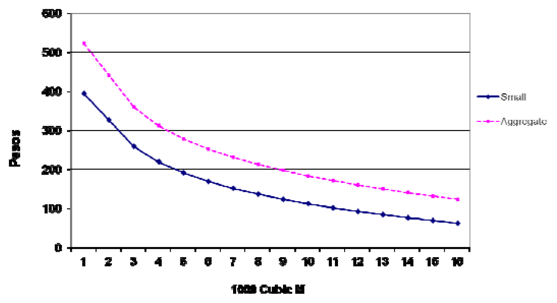
To compare the aggregate and disaggregate water demand functions, we plot the disaggregated and aggregated estimated functions over the same range of potential water reductions. The functions can be thought of as measuring the impact of a water tax policy or the cost of a quantitative reallocation.
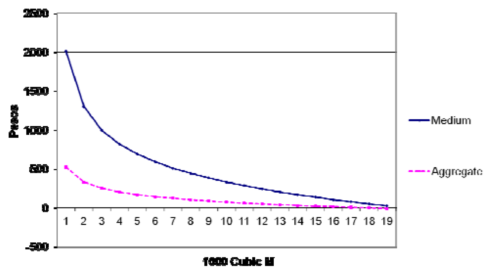
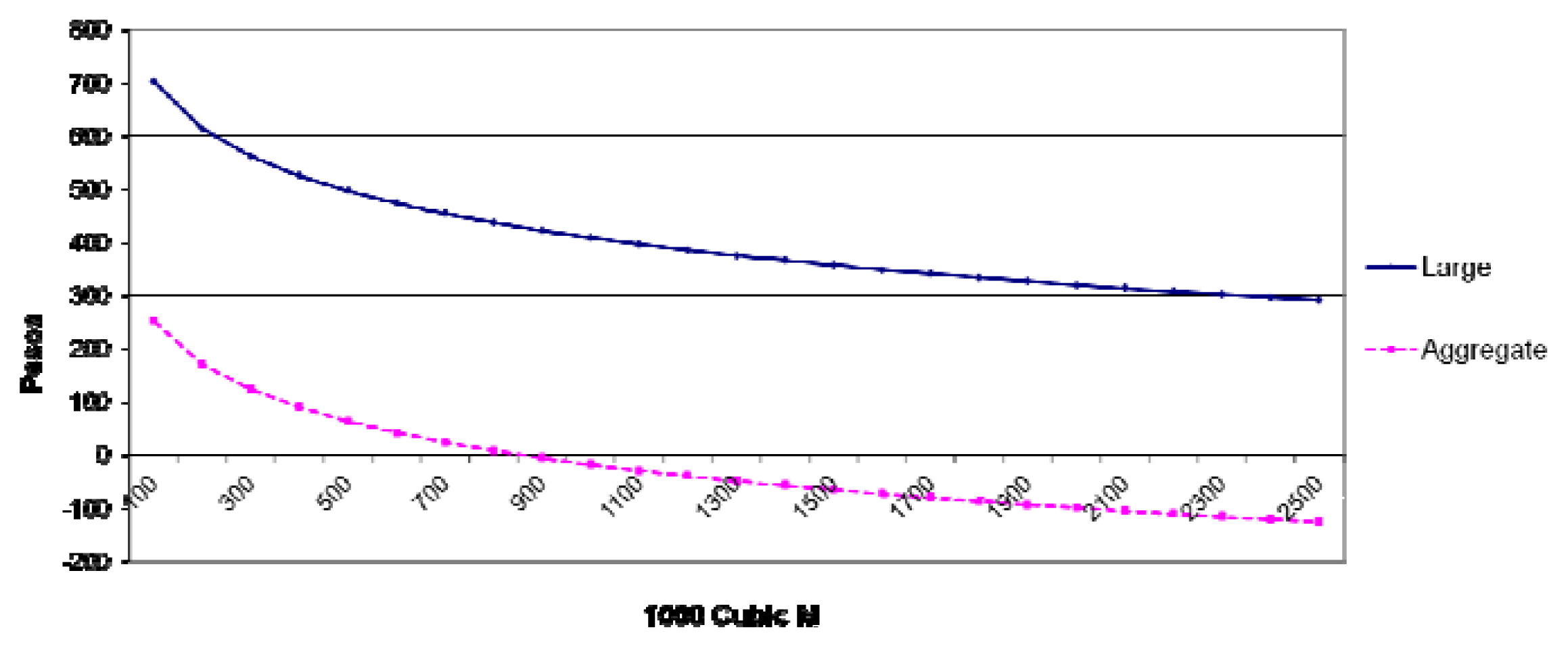
Figures 1–3 show the functions.
Figure 1 presents the functions for the aggregated and small farms. The aggregate function most closely approximates the small-farm function in that the difference is a constant overvaluation of water, which would introduce a constant distortion into policies.
Figure 2 compares functions for aggregated and medium farms and demonstrates very large undervaluations over most of the water-quantity range. The demands coincide at large quantities but differ in value by a factor of four at very small quantities. Thus, the stronger the policy, the greater the undervaluation.
Figure 3 compares the functions of large farms and the aggregated sample. Due to bias toward small farms in the aggregate set of farms with binding water constraints, the aggregate function undervalues the large-farm data so badly that it is unusable for policy analysis.
The results in Figures 1–3 clearly show that, despite similarity in the interval elasticities, the water demand function estimated using the aggregate data set is unusable for the large-farm group and has the expected upward and downward bias in the small- and medium-farm groups, respectively. For this empirical example, estimation of policy models disaggregated by farm size gains significantly more from the reduction of aggregation bias than it loses from small-sample imprecision.
5. Conclusions
This paper shows that a GME approach makes it is possible to construct flexible-form production function models from a data set of modest size. A researcher can construct similar, theoretically consistent, flexible-form production models using data ranging from small samples with minimal degrees of freedom to full econometric data sets with standard degrees of freedom. The convergence of GME estimates to conventional estimates as sample size increases means that expansion of the data set will generate a continuum from an optimization to an econometric model.
The disaggregate production models yield all of the comparative static properties and parameters of large-sample models. The effect of any constraint on inputs is directly incorporated in the estimates through simultaneous estimation of shadow values of the allocatable resources. Models of production functions are advantageous because they are readily understood by members of other scientific disciplines (especially those who model biophysical processes), who thus can add useful information that will clarify prior support values or constraints to production.
In this example, the aggregation bias in the aggregated model swamped any gains from reducing small-sample error. The disaggregated model yielded greater precision for a regional data set. This gain from disaggregation of production models will require substantial additional testing before we can conclude that it is a common phenomenon. In this example, the empirical results show that the disaggregated and aggregated estimates similarly and relatively accurately reproduce the actual production system as measured by the values of the R-squared, absolute deviation, and the entropy information index. Despite similar estimates of the elasticity of water demand, the disaggregated samples showed a wide variation in the derived demand for water that would directly influence farm-level responses to policy changes (such as in the price of water, for example). The utility of undertaking a rigorous disaggregation of production function estimates is clearly demonstrated by the results, and should serve as an encouragement to other researchers who wish to look more closely at the heterogeneity in producer behavior that almost certainly exists across the farm landscape in other parts of the world.
Acknowledgments
The authors gratefully acknowledge the cooperation of Musa Asad at the World Bank and Ariel Dinar at University of California, Riverside, USA.
Conflicts of Interest
The authors declare no conflict of interest.
- Author ContributionsThe authors made equal contributions to the design, analysis, and writing of the paper. Both authors read and approved the final manuscript.
References
- Antle, J.M.; Capalbo, S. Econometric-Process Models of Production. Am. J. Agr. Econ 2001, 83, 389–401. [Google Scholar]
- Just, R.E.; Antle, J.M. Interactions between Agricultural and Environmental Policies: A Conceptual Framework. Am. Econ. Rev 1990, 80, 197–202. [Google Scholar]
- Lence, S.H.; Miller, D.J. Recovering Output-specific Inputs from Aggregate Input Data: A Generalized Cross-Entropy Approach. Am. J. Agr. Econ 1998, 80, 852–867. [Google Scholar]
- Lansink, A.O.; Silva, E.; Stefanou, S. Inter-Firm and Intra-Firm Efficiency Measures. J. Prod. Anal 2001, 15, 185–199. [Google Scholar]
- Golan, A.; Judge, G.; Robinson, S. Recovering Information from Incomplete or Partial Multisectoral Economic Data. Rev. Econ. Stat 1994, 76, 541–549. [Google Scholar]
- Golan, A.; Judge, G.; Perloff, J. Estimating the Size Distribution of Firms Using Government Summary Statistics. J. Ind. Econ 1996, 44, 69–80. [Google Scholar]
- Mittelhammer, R.C.; Cardell, N.C.; Marsh, T.L. The Data-constrained Generalized Maximum Entropy Estimator of the GLM: Asymptotic Theory and Inference. Entropy 2013, 15, 1756–1775. [Google Scholar]
- Golan, A.; Judge, G.; Miller, D. Maximum Entropy Econometrics: Robust Estimation with Limited Data; Wiley: Chichester, UK, 1996. [Google Scholar]
- Zhang, X.; Fan, S. Crop-specific Production Technologies in Chinese Agriculture. Am. J. Agr. Econ 2001, 83, 378–388. [Google Scholar]
- Lence, S.H.; Miller, D.J. Estimation of Multi-Output Production Functions with Incomplete Data: A Generalized Maximum Entropy Approach. Eur. Rev. Agr. Econ 1998, 25, 188–209. [Google Scholar]
- Heckelei, T.; Wolff, H. Estimation of Constrained Optimization Models for Agricultural Supply Analysis Based on Generalized Maximum Entropy. Eur. Rev. Agr. Econ 2003, 30, 27–50. [Google Scholar]
- Efron, B.; Tibsharani, J. An Introduction to the Bootstrap; Chapman & Hall: London, UK, 1993. [Google Scholar]
- Love, H.A. Conflicts between Theory and Practice in Production Economics. Am. J. Agr. Econ 1999, 81, 696–702. [Google Scholar]
- Just, R.E.; Zilberman, D.; Hochman, E. Estimation of Multicrop Production Functions. Am. J. Agr. Econ 1983, 65, 770–780. [Google Scholar]
- McCarl, B.A.; Adams, D.M.; Alig, R.J.; Chmelik, J.T. Analysis of Biomass Fueled Electrical Power Plants: Implications in the Agricultural and Forestry Sectors. Ann. Oper. Res 2000, 94, 37–55. [Google Scholar]
- Alig, R.J.; Adams, D.M.; McCarl, B.A. Impacts of Incorporating Land Exchanges between Forestry and Agriculture in Sector Models. J. Agr. Appl. Econ 1998, 30, 389–401. [Google Scholar]
- United States, Bureau of Reclamation, Central Valley Project Improvement Act: Draft Programmatic Environmental Impact Statement; U.S. Department of the Interior, Bureau of Reclamation: Washington, DC, USA, 1997.
- Wu, J.J.; Babcock, B. Meta-modeling Potential Nitrate Water Pollution in the Central United States. J. Environ. Qual 1999, 28, 1916–1928. [Google Scholar]
- Mendelsohn, R.; Nordhaus, W.D.; Shaw, D. The Impact of Global Warming on Agriculture: A Ricardian Analysis. Am. Econ. Rev 1994, 84, 753–771. [Google Scholar]
- Antle, J.M.; Valdivia, R.O. Modelling the Supply of Ecosystem Services from Agriculture: A Minimum-data Approach. Aust. J. Agr. Resour. Econ 2006, 50, 1–15. [Google Scholar]
- Howitt, R.E. Positive Mathematical Programming. Am. J. Agr. Econ 1995, 77, 329–342. [Google Scholar]
- Brooke, A.; Kendrick, D.; Meeraus, A. GAMS: A User’s Guide; Associated Computing Machinery/The Scientific Press: New York, NY, USA, 1988. [Google Scholar]
- Soofi, E.S. Capturing the Intangible Concept of Information. J. Am. Stat. Assoc 1994, 89, 1243–1254. [Google Scholar]
- Guevara-Sanginés, A. Case Study: Water Subsidies and Aquifer Depletion in Mexico’s Arid Regions; Occasional Paper 23; Human Development Report Office, United Nations Development Program: New York, NY, USA, 2006. [Google Scholar]


| Farm Size | Small | Medium | Large | Summary | ||||
|---|---|---|---|---|---|---|---|---|
| Crop | Cultivated land (ha) | water used (m3/ha) * | Cultivated land (ha) | water used (m3/ha) * | Cultivated land (ha) | water used (m3/ha) * | Cultivated land (ha) | water used (m3/ha) * |
| Alfalfa | 1.5 | 23,000 | 10.0 | 16,000 | 129.0 | 18,558 | 140.5 | 19,186 |
| Wheat | 19.4 | 5,000 | 77.0 | 5,000 | 96.4 | 5,000 | ||
| Maize | 3.0 | 8,000 | 50.1 | 5,325 | 1,358.3 | 5,236 | 1,411.4 | 6,187 |
| Cotton | 290.0 | 8,138 | 290.0 | 8,138 | 324.0 | 8,069 | ||
| Melon | 10.0 | 17,000 | 180.0 | 2,600 | 190.0 | 9,800 | ||
| Sweet Potato | 20.0 | 7,000 | 20.0 | 7,000 | ||||
| Beans | 0.5 | 5,000 | 0.5 | 5,000 | ||||
| Sorghum | 15.0 | 7,600 | 83.0 | 4,172 | 2,198.0 | 2,023 | 2,296.0 | 4,598 |
| Average | 30.0 | 12,120 | 196.5 | 7,699 | 4,252.3 | 6,936 | 4,478.8 | 8,105 |
*Average of water used per hectare.
| Field | Forage | Maize | Sorghum | Wheat | |
|---|---|---|---|---|---|
| All farms | 0.369 | 0.431 | 0.658 | 0.67 | 0.402 |
| Small farms | 0.385 | 0.444 | 0.411 | 0.615 | |
| Medium farms | 0.511 | 0.437 | |||
| Large farms | 0.387 | 0.39 |
| Field | Forage | Maize | Sorghum | Wheat | |
|---|---|---|---|---|---|
| All farms | 0.721 | 0.729 | 0.397 | 0.761 | 0.713 |
| Small farms | 0.720 | 0.726 | 0.709 | 0.702 | - |
| Medium farms | - | - | 0.699 | 0.697 | - |
| Large farms | - | - | 0.714 | 0.718 | - |
| Field | Forage | Maize | Sorghum | Wheat | |
|---|---|---|---|---|---|
| All farms | 0.375 | 0.369 | 0.269 | 0.319 | 0.528 |
| Small farms | 0.374 | 0.393 | 0.299 | 0.142 | |
| Medium farms | 0.696 | 0.263 | |||
| Large farms | 0.190 | 0.290 |
| Field | Forage | Maize | Sorghum | Wheat | |
|---|---|---|---|---|---|
| All farms | 3.680 | 6.550 | 40.000 | 40.870 | 1.50 |
| Small farms | 5.549 | 15.102 | 24.495 | 37.518 | |
| Medium farms | 16.797 | 37.749 | |||
| Large farms | 9.319 | 12.712 |
| Land Cost | Water Cost | |||
|---|---|---|---|---|
| Shadow Value | Nominal Cost | Shadow Value | Nominal Cost | |
| Small farms | 959.82 | 762.00 | 255.59 | 222.02 |
| Medium farms | 1,947.57 | 637.10 | 855.28 | 185.85 |
| Large farms | 1,208.32 | 977.27 | 223.56 | 223.06 |
| Small Farm | Medium Farm | Large Farm | ||||
|---|---|---|---|---|---|---|
| Mean | Variance | Mean | Variance | Mean | Variance | |
| RTS | 0.615 | 0.0200 ** | 0.437 | 0.017 | 0.390 | 0.056 * |
| Substitution | 0.615 | 0.263 | 0.688 | 0.019 ** | 0.717 | 0.158 * |
| Scale | 8.552 | 251.250 | 48.445 | 256,863.530 | 125.500 | 28,102.500 |
**significant at 1%;*significant at 5%.
| Small–Medium | Small–Large | Medium–Large | |
|---|---|---|---|
| Return to scale | 2.578 ** | 2.721 ** | 0.440 |
| Substitution | −0.338 | −0.494 | −0.170 |
| Scale | −0.276 | −2.423 ** | −0.423 |
**significant at 1%;*significant at 5%.
| Farm Size | Demand Equation | R-square |
|---|---|---|
| Small | P = 618.65 − 97.63 Ln(Q) | 0.78 |
| Medium | P = 3,024.2 − 440.54 Ln(Q) | 0.74 |
| Large | P = 1,290.4 − 127.69 Ln(Q) | 0.33 |
| Aggregate | P = 792.61 − 117.37 Ln(Q) | 0.75 |
© 2014 by the authors; licensee MDPI, Basel, Switzerland This article is an open access article distributed under the terms and conditions of the Creative Commons Attribution license (http://creativecommons.org/licenses/by/3.0/).
Share and Cite
Howitt, R.E.; Msangi, S. Entropy Estimation of Disaggregate Production Functions: An Application to Northern Mexico. Entropy 2014, 16, 1349-1364. https://doi.org/10.3390/e16031349
Howitt RE, Msangi S. Entropy Estimation of Disaggregate Production Functions: An Application to Northern Mexico. Entropy. 2014; 16(3):1349-1364. https://doi.org/10.3390/e16031349
Chicago/Turabian StyleHowitt, Richard E., and Siwa Msangi. 2014. "Entropy Estimation of Disaggregate Production Functions: An Application to Northern Mexico" Entropy 16, no. 3: 1349-1364. https://doi.org/10.3390/e16031349