An Entropy Measure of Non-Stationary Processes


Abstract
: Shannon’s source entropy formula is not appropriate to measure the uncertainty of non-stationary processes. In this paper, we propose a new entropy measure for non-stationary processes, which is greater than or equal to Shannon’s source entropy. The maximum entropy of the non-stationary process has been considered, and it can be used as a design guideline in cryptography.1. Introduction
Information science considers an information process, uses the probability measure for random states and Shannon’s entropy as the uncertainty function of these states [1–3]. For a stationary source, the probability and the Shannon’s entropy can be determined by using statistical physics methods, while for a non-stationary source, all the statistical physics methods fail, thus the Shannon entropy measure may not be available. Till now, the entropy of non-stationary process is still not fully understood, except for some specific types of non-stationary process [4] that use the following entropy formula to measure the uncertainty:
This kind of non-stationary process requires a known probability function, and the probability function is deterministically varied. This formula will fail if the probability function of the non-stationary process is stochastically varied. For a non-stationary process, if its parametric is a stationary random variable, then this kind of non-stationary process can be considered as a piecewise stationary process, and many papers use the following source entropy formula, proposed by Shannon, to measure the uncertainty [5–9]:
where for each possible state i there will be a set of probabilities pi(j) of producing the various possible symbols j.
In this paper, we will consider the non-stationary process, with its parametric be a stationary random variable. We will show that the entropy of this kind of non-stationary process should not be measured by Shannon’s source entropy (Equation (2)). Actually, Shannon’s source entropy Equation (2) is only used for a stationary process with multiple-states, not for non-stationary processes. In our paper, we will propose an entropy formula to measure the uncertainty of non-stationary processes. Our entropy measure is greater than or equal to Shannon’s source entropy formula. These two measures are equal if and only if the process is stationary. Our entropy measure can be used as a complexity criterion of non-stationary processes and as a design guideline for cryptographic uses.
The rest of this paper is organized as follows: Section 2 shows that Shannon’s source entropy formula is not appropriate to measure the uncertainty of non-stationary processes. In Section 3, a new entropy formula is proposed to measure the uncertainty of non-stationary processes and some properties are presented. In Section 4, the maximum entropy of the non-stationary process is considered. Section 5 concludes the paper.
2. The Limitation of Shannon’s Source Entropy in Non-Stationary Process
First, let’s consider the following two examples, one is for discrete source and the other is for continuous source:
Example 1. Consider a discrete source of two kinds of symbol 0 and 1. This discrete source varies between the states “1” and “2” randomly with probabilities P1 = 0.2 and P2 = 0.8. For state “1”, the probability of producing the symbol 0 is 0.4, and producing the symbol 1 is 0.6. For state “2”, the probability of producing the symbol 0 is 0.3, and producing the symbol 1 is 0.7. Obviously, this discrete source is non-stationary. By using Shannon’s source entropy Equation (2), we have H = 0.6233. By calculating the entropy of the 01 sequences which generated by this discrete source, we have H approaches to 0.629 with the sequence length increased, which is bigger than Shannon’s source entropy measure.
Example 2. Consider a continuous source of a parameter-varied normal distribution N(μ, 1), which parameter μ varies between μ1, μ2, …, μn randomly with probabilities p1, p2, … ,pn. Obviously, this continuous source is non-stationary. By using Shannon’s source entropy Equation (2), we have H = 0.5ln2πe, which is not relevant to μ. Then, the uncertainty of this non-stationary source equals to the uncertainty of normal distribution source with fixed μ as N(0, 1), which is not convinced (the variation of parameter μ also brings some of uncertainty when determining the states).
Therefore, Shannon’s source entropy formula is not appropriate to measure the uncertainty of a non-stationary process. The entropy of non-stationary processes is always bigger than Shannon’s source entropy measure. Next, we will analyze why this happens.
Let s1s2…si(1)si(1)+1…si(2)si(2)+1…sN be a symbol sequence generated by the source of Example 3, which s1s2…si(1) is generated by a fixed random parameter, si(1)+1…si(2) is generated by a fixed random parameter, and so on. For the first symbol s1, its uncertainty can be written as h(p) o H1. Here, h(p) is the uncertainty of varying parameter, and H1 is the uncertainty of symbol s1 with a known parameter. “o” is an operator which has the following properties:
- (1)
0 o a = a.
- (2)
a o b = b o a ≥ max(a, b).
- (3)
a o b = a if and only if b = 0.
For the symbol s2, its uncertainty is H2, without h(p) for its parameter is determined. For the symbol si(1)+1, its uncertainty is h(p) o Hi(1)+1, …. Then the average uncertainty of this non-stationary source can be written as:
here, E|si(j)+1…si(j+1)| is the average length of symbol sequence by each parameter. The “=” holds if and only if the source is stationary, which degenerate to Shannon’s source entropy measure.
3. The Entropy of Non-Stationary Process and Its Properties
According to the Boltzmann-Gibbs theorem, we should consider all the possible states and their probabilities when we measure the uncertainty of a source. Consider a non-stationary process which varies randomly in n kinds of possible states. The probabilities of each states are p1, p2, …, and pn respectively. For the state i, the output variable satisfies the probability density function fi. The probability of generating a N-length sequence by this non-stationary source is:
Then, the uncertainty of the N-length sequence is:
The average uncertainty of this non-stationary process is:
Theorem 1.
Proof
First, we consider the case N = 2. We have:
Assume the equation holds when N = k. Then for N = k + 1, denote , then we have:
Thus, concluding our proof.
According to Equations (5) and (6) and theorem 1, the entropy of the non-stationary process can be written as:
Equation (7) is the entropy formula of the non-stationary process when the states vary discretely. For a continuously case, the entropy formula can be written as:
Here, g(y) is the probability density function of the varying state and fy is the probability density function of the output variable for each state y. We have that by using the entropy equations (7) and (8) instead of Shannon’s source entropy, there are no such inconsistencies as proposed in examples 1 and 2.
Theorem 2
Let HS and H be the Shannon’s entropy measure and our entropy measure of a non-stationary process respectively, H(p) be the Shannon’s entropy of the varying states. We have the following inequality hold:
Proof
We use Equation (7) as our entropy formula (states vary discretely). For the continuous case, it can be proven similarly.
We consider H – Hs, and have:
Due to , we have:
Thus, we have H < Hs + H(p). Additionally, consider the following functional F:
It is easily to prove that functional F reaches its minimum when f1 = f2 = … = fn, we have:
Thus, we have H ≥ Hs, which concluding our proof.
Theorem 2 shows that the entropy of non-stationary process is greater than or equal to the Shannon’s entropy measure. These two measures are equal if and only if the process is stationary. Furthermore, H < Hs + H(p) means that the entropy of non-stationary process cannot be written as the sum of Hs and H(p), although its uncertainty is brought by these the aspects. In another word, they are not independent of each other.
4. Maximum Entropy and Its Application in Cryptography
In recent years, chaotic systems were regarded as an important pseudorandom source in the design of random number generators [10–12]. As we know, chaotic systems may be attacked by phase space reconstruction and nonlinear prediction techniques. If the system is abiding references [13–15] propose a chaotic system with varying parameters to resist these attacks. However, the varying method is rather simple. A more secure method is to vary the parameters in a random-like way, then the output sequence come to be non-stationary. Entropy is an important criterion in cryptographic use. With our entropy formula of non-stationary process, we can compare the different varying methods and guide us to design a varying method in order to make the entropy maximum. It can be expressed as the following mathematical problem.
P1
The maximum of functional:
under the condition and 0 ≤ pi ≤ 1.
Design a Lagrange functional:
Solve the following equations:
Compare these extreme values in order to get the maximum entropy and the corresponding pi.
Consider the discrete case (the output variables of each states are discrete). Assume the non-stationary process is varying in n kinds of possible states a1, a2, … , an with probabilities p1, p2, … , pn. For each state ai, the output variables are b1, b2, … , bN and the probabilities are fi1, fi2, … , fiN respectively. Then, the entropy of this non-stationary process is:
By using the above Lagrange method, we have that the entropy (9) reach its maximum value when the following equation holds:
The maximum entropy is logN which equals to the stationary uniform distribution.
For the continuous case (the output variables of each states are continuous), the method is similar. Next, we show two simple examples.
Example 3. Consider a non-stationary process which varies between two possible states a1 and a2 with probabilities p1 and p2 respectively. For state a1, the output variables are b1 and b2 with probabilities f11 = 0.75 and f12 = 0.25. For state a2, the output variables are b1 and b2 with probabilities f21 = 1/3 and f22 = 2/3. By solving the maximum entropy problem, we have that the entropy reaches its maximum value when p1 = 0.4, p2 = 0.6, and Hmax = log2.
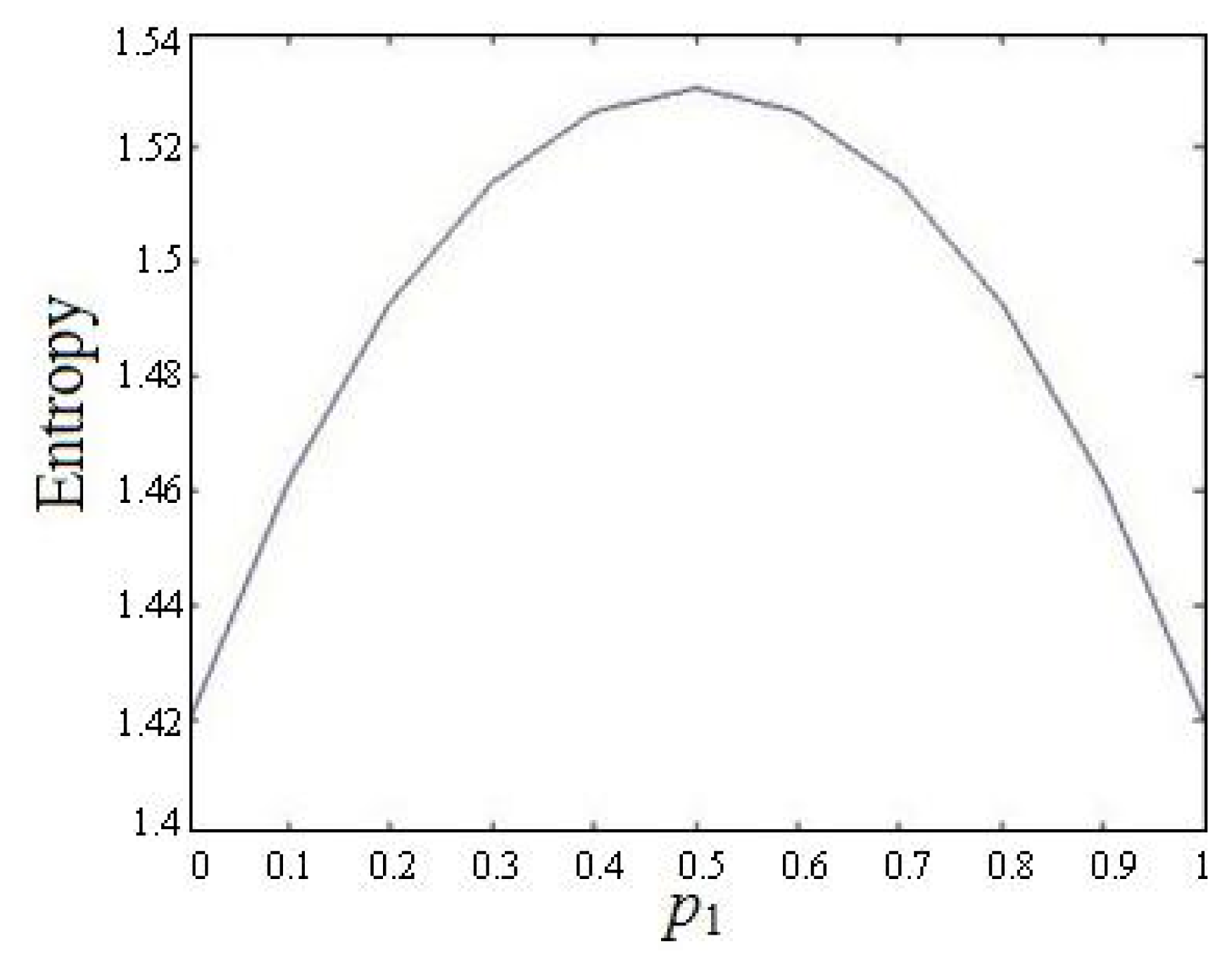
Example 4. Consider a non-stationary process which varies in two states a1 and a2 with probabilities p1 and p2 respectively. For state a1, the output variables satisfy the normal distribution N(0, 1). For state a2, the output variables satisfy the normal distribution N(1, 1). By solving the maximum entropy problem, we have that the entropy reaches its maximum value when p1 = 0.5, and Hmax = 1.5304. Figure 1 shows the relation between the Entropy and p1.
5. Conclusions
In this paper, we first prove that Shannon’s source entropy is not appropriate to measure the uncertainty of non-stationary processes. Then, we propose an entropy formula to measure the uncertainty of such non-stationary processes. Our entropy measure is greater than or equal to Shannon’s source entropy formula. These two measures are equal if and only if the process is stationary. Furthermore, we study the maximum entropy of our entropy formula. The maximum entropy can be used as a guideline for constructing a non-stationary source in cryptographic uses.
Acknowledgments
This work was supported in part by the National Natural Science Foundation of China under Grant 60773192, in part by the National High-Tech Research and Development Program of China (863) under Grant 2006AA01Z426, and in part by the 12th Five-year National Code Development Fund under Grant MMJJ201102016.
Conflicts of Interest
The authors declare no conflict of interest.
- Author ContributionsLing Feng Liu did the theoretical work and wrote this paper; Han Ping Hu proposed this idea and checked the whole paper; Ya Shuang Deng and Nai Da Ding helped in the theoretical work.
References
- Shannnon, C.E.; Weaver, W. The Mathematical Theory of Communication; University of Illinois Press: Urbana, IL, USA, 1949. [Google Scholar]
- Jaynes, E.T. Information Theory and Statistical Mechanics in Statistical Physics; Benjamin, Inc: New York, NY, USA, 1963; p. 181. [Google Scholar]
- Kolmogorov, A.N. Logical basis for information theory and probability theory. IEEE Trans. Inform. Theory 1968, 14, 662–664. [Google Scholar]
- Katz, A. Principles of statistical mechanics: The information theory approach; W.H. Freeman and Company: San Francisco, CA, USA, 1967. [Google Scholar]
- Karaca, M.; Alpcan, T.; Ercetin, O. Smart Scheduling and Feedback Allocation over Non-stationary Wireless Channels. ICC 2012, 6586–6590. [Google Scholar]
- Olivares, F.; Plastino, A.; Rosso, O.A. Contrasting chaos with noise via local versus global information quantifiers. Phys. Lett. A 2012, 376, 1577–1583. [Google Scholar]
- Reif, J.H.; Storer, J.A. Optimal encoding of non-stationary sources. Inform. Sci 2001, 135, 87–105. [Google Scholar]
- Ray, A.; Chowdhury, A.R. On the characterization of non-stationary chaotic systems: Autonomous and non-autonomous cases. Phys. A 2010, 389, 5077–5083. [Google Scholar]
- He, K.F.; Xiao, S.W.; Wu, J.G.; Wang, G.B. Time-Frequency Entropy Analysis of Arc Signal in Nom-Stationary Submerged Arc Welding. Engineering 2011, 3, 105–109. [Google Scholar]
- Kocarev, L.; Jakimoski, G. Pseudorandom bits generated by chaotic maps. IEEE Trans. Circ. Syst. Fund. Theor. Appl 2003, 50, 123–126. [Google Scholar]
- Huaping, L.; Wang, S.; Gang, H. Pseudo-random number generator based on coupled map lattices. Int. J. Mod. Phys. B 2004, 18, 2409–2414. [Google Scholar]
- Kanso, A.; Smaoui, N. Logistic chaotic maps for binary numbers generations. Chaos Solitons Fractals 2009, 40, 2557–2568. [Google Scholar]
- Prokhorov, M.D.; Ponomarenko, V.I.; Karavaev, A.S.; Bezruchko, B.P. Reconstruction of time-delayed feedback systems from time series. Physica D 2005, 203, 209–223. [Google Scholar]
- Cohen, A.B.; Ravoori, B.; Murphy, T.E.; Roy, R. Using Synchronization for Prediction of High-Dimensional Chaotic Dynamics. Phys. Rev. Lett 2008, 154102. [Google Scholar]
- Jing, M.; Chao, T.; Huan, D.G. Synchronization of the time-varying parameter chaotic system and its application to secure communication. Chinese Phys 2003, 12, 381–388. [Google Scholar]

© 2014 by the authors; licensee MDPI, Basel, Switzerland This article is an open access article distributed under the terms and conditions of the Creative Commons Attribution license (http://creativecommons.org/licenses/by/3.0/).
Share and Cite
Liu, L.F.; Hu, H.P.; Deng, Y.S.; Ding, N.D. An Entropy Measure of Non-Stationary Processes. Entropy 2014, 16, 1493-1500. https://doi.org/10.3390/e16031493
Liu LF, Hu HP, Deng YS, Ding ND. An Entropy Measure of Non-Stationary Processes. Entropy. 2014; 16(3):1493-1500. https://doi.org/10.3390/e16031493
Chicago/Turabian StyleLiu, Ling Feng, Han Ping Hu, Ya Shuang Deng, and Nai Da Ding. 2014. "An Entropy Measure of Non-Stationary Processes" Entropy 16, no. 3: 1493-1500. https://doi.org/10.3390/e16031493