Quantifying Unique Information


Abstract
: We propose new measures of shared information, unique information and synergistic information that can be used to decompose the mutual information of a pair of random variables (Y, Z) with a third random variable X. Our measures are motivated by an operational idea of unique information, which suggests that shared information and unique information should depend only on the marginal distributions of the pairs (X, Y ) and (X, Z). Although this invariance property has not been studied before, it is satisfied by other proposed measures of shared information. The invariance property does not uniquely determine our new measures, but it implies that the functions that we define are bounds to any other measures satisfying the same invariance property. We study properties of our measures and compare them to other candidate measures.MSC Classification: 94A15, 94A171. Introduction
Consider three random variables X, Y, Z with finite state spaces
 ,
,  ,
,  . Suppose that we are interested in the value of X, but we can only observe Y or Z. If the tuple (Y, Z) is not independent of X, then the values of Y or Z or both of them contain information about X. The information about X contained in the tuple (Y, Z) can be distributed in different ways. For example, it may happen that Y contains information about X, but Z does not, or vice versa. In this case, it would suffice to observe only one of the two variables Y, Z namely the one containing the information. It may also happen that Y and Z contain different information, so it would be worthwhile to observe both of the variables. If Y and Z contain the same information about X, we could choose to observe either Y or Z. Finally, it is possible that neither Y nor Z taken for itself contains any information about X, but together they contain information about X. This effect is called synergy, and it occurs, for example, if all variables X, Y, Z are binary, and X = Y XORZ. In general, all effects may be present at the same time. That is, the information that (Y, Z) has about X is a mixture of shared information SI(X : Y ; Z) (that is, information contained both in Y and in Z), unique information UI(X : Y \Z) and UI(X : Z\Y ) (that is, information that only one of Y and Z has) and synergistic or complementary information CI(X : Y ; Z) (that is, information that can only be retrieved when considering Y and Z together).
The total information that (Y, Z) has about X can be quantified by the mutual information MI(X : (Y, Z)). Decomposing MI(X : (Y, Z)) into shared information, unique information and synergistic information leads to four terms, as:
The interpretation of the four terms as information quantities demands that they should all be positive. Furthermore, it suggests that the following identities also hold:
In the following, when we talk about a bivariate information decomposition, we mean a set of three functions SI, UI and CI that satisfy (1) and (2).
Combining the three equalities in (1) and (2) and using the chain rule of mutual information:
yields the identity:
which identifies the co-information with the difference of shared information and synergistic information (the co-information was originally called interaction information in [1], albeit with a different sign in the case of an odd number of variables). It has been known for a long time that a positive co-information is a sign of redundancy, while a negative co-information expresses synergy [1]. However, although there have been many attempts, as of currently, there has been no fully satisfactory solution to separate the redundant and synergistic contributions to the co-information, and also, a fully satisfying definition of the function UI is still missing. Observe that, since we have three equations ((1) and (2)) relating the four quantities SI(X : Y ; Z), UI(X : Y \ Z), UI(X : Z \ Y ) and CI(X : Y ; Z), it suffices to specify one of them to compute the others. When defining a solution for the unique information UI, this leads to the consistency equation:
The value of (4) can be interpreted as the union information, that is, the union of the information contained in Y and in Z without the synergy.
The problem of separating the contributions of shared information and synergistic information to the co-information is probably as old as the definition of co-information itself. Nevertheless, the co-information has been widely used as a measure of synergy in the neurosciences; see, for example, [2,3] and the references therein. The first general attempt to construct a consistent information decomposition into terms corresponding to different combinations of shared and synergistic information is due to Williams and Beer [4]. See also the references in [4] for other approaches to study multivariate information. While the general approach of [4] is intriguing, the proposed measure of shared information Imin suffers from serious flaws, which prompted a series of other papers trying to improve these results [5–7].
In our current contribution, we propose to define the unique information as follows: Let Δ be the set of all joint distributions of X, Y and Z. Define:
as the set of all joint distributions that have the same marginal distributions on the pairs (X, Y ) and (X, Z). Then, we define:
where MIQ(X : Y |Z) denotes the conditional mutual information of X and Y given Z, computed with respect to the joint distribution Q. Observe that:
where the chain rule of mutual information was used. Hence, satisfies the consistency Condition (4), and we can use (2) and (3) to define corresponding functions and , such that and form a bivariate information decomposition. and are given by:
In Section 3, we show that and are non-negative, and we study further properties. In Appendix A.1, we describe ΔP, in terms of a parametrization.
Our approach is motivated by the idea that unique and shared information should only depend on the marginal distribution of the pairs (X, Z) and (X, Y ). This idea can be explained from an operational interpretation of unique information: Namely, if Y has unique information about X (with respect to Z), then there must be some way to exploit this information. More precisely, there must be a situation in which Y can use this information to perform better at predicting the outcome of X. We make this idea precise in Section 2 and show how it naturally leads to the definitions of and as given above. Section 3 contains basic properties of these three functions. In particular, Lemma 5 shows that all three functions are non-negative. Corollary 7 proves that the interpretation of as unique information is consistent with the operational idea put forward in Section 2. In Section 4, we compare our functions with other proposed information decompositions. Some examples are studied in Section 5. Remaining open problems are discussed in Section 6. Appendices A.1 to A.3 discuss more technical aspects that help to compute and .
After submitting our manuscript, we learned that the authors of [5] had changed their definitions in Version 5 of their preprint. Using a different motivation, they define a multivariate measure of union information that leads to the same bivariate information decomposition.
2. Operational Interpretation
Our basic idea to characterize unique information is the following: If Y has unique information about X with respect to Z, then there must be some way to exploit this information. That is, there must be a situation in which this unique information is useful. We formalize this idea in terms of decision problems as follows:
Let X, Y, Z be three random variables; let p be the marginal distribution of X, and let κ ∈
 and μ ∈
 be (row) stochastic matrices describing the conditional distributions of Y and Z, respectively, given X. In other words, p, κ and μ satisfy:
Observe that, if p(x) > 0, then κ(x; y) and μ(x; z) are uniquely defined. Otherwise, κ(x; y) and μ(x; z) can be chosen arbitrarily. In this section, we will assume that the random variable X has full support. If this is not the case, our discussion will remain valid after replacing
by the support of X. In fact, the information quantities that we consider later will not depend on those matrix elements κ(x; y) and μ(x; z) that are not uniquely defined.
Suppose that an agent has a finite set of possible actions
 . After the agent chooses her action a ∈
, she receives a reward u(x, a), which not only depends on the chosen action a ∈
, but also on the value x ∈
of the random variable X. The tuple (p, , u), consisting of the prior distribution p, the set of possible actions A and the reward function u, is called a decision problem. If the agent can observe the value x of X before choosing her action, her best strategy is to chose a in such a way that u(x, a) =
. After the agent chooses her action a ∈
, she receives a reward u(x, a), which not only depends on the chosen action a ∈
, but also on the value x ∈
of the random variable X. The tuple (p, , u), consisting of the prior distribution p, the set of possible actions A and the reward function u, is called a decision problem. If the agent can observe the value x of X before choosing her action, her best strategy is to chose a in such a way that u(x, a) =
 u(x, a′). Suppose now that the agent cannot observe X directly, but the agent knows the probability distribution p of X. Moreover, the agent observes another random variable Y, with conditional distribution described by the row-stochastic matrix κ ∈
. In this context, κ will also be called a channel from
to
. When using a channel κ, the agent’s optimal strategy is to choose her action in such a way that her expected reward:
u(x, a′). Suppose now that the agent cannot observe X directly, but the agent knows the probability distribution p of X. Moreover, the agent observes another random variable Y, with conditional distribution described by the row-stochastic matrix κ ∈
. In this context, κ will also be called a channel from
to
. When using a channel κ, the agent’s optimal strategy is to choose her action in such a way that her expected reward:
is maximal. Note that, in order to maximize (5), the agent has to know (or estimate) the prior distribution of X, as well as the channel κ. Often, the agent is allowed to play a stochastic strategy. However, in the present setting, the agent cannot increase her expected reward by randomizing her actions; and therefore, we only consider deterministic strategies here.
Let R(κ, p, u, y) be the maximum of (5) (over a ∈
), and let:
be the maximal expected reward that the agent can achieve by always choosing the optimal action.
In this setting, we make the following definition:
Definition 1
Let X, Y, Z be three random variables; and let p be the marginal distribution of X, and let κ ∈
and μ ∈
be (row) stochastic matrices describing the conditional distributions of Y and Z, respectively, given X.
Y has unique information about X (with respect to Z), if there is a set
![Entropy 16 02161f8]() and a reward function u ∈
and a reward function u ∈
![Entropy 16 02161f10]() that satisfy R(κ, p, u) > R(μ, p, u).
that satisfy R(κ, p, u) > R(μ, p, u).Z has no unique information about X (with respect to Y ), if for any set
![Entropy 16 02161f8]() and reward function u ∈
and reward function u ∈
![Entropy 16 02161f10]() , the inequality R(κ, p, u) ≥ R(μ, p, u) holds. In this situation we also say that Y knows everything that Z knows about X, and we write Y ⊒X Z.
, the inequality R(κ, p, u) ≥ R(μ, p, u) holds. In this situation we also say that Y knows everything that Z knows about X, and we write Y ⊒X Z.

This operational idea allows one to decide when the unique information vanishes, but, unfortunately, does not allow one to quantify the unique information.
As shown recently in [8], the question whether or not Y ⊒X Z does not depend on the prior distribution p (but just on the support of p, which we assume to be
). In fact, if p has full support, then, in order to check whether Y ⊒X Z, it suffices to know the stochastic matrices κ, μ representing the conditional distributions of Y and Z, given X.
Consider the case
=
and κ = μ ∈ K(
;
), i.e., Y and Z use a similar channel. In this case, Y has no unique information with respect to Z, and Z has no unique information with respect to Y. Hence, in the decomposition (1), only the shared information and the synergistic information may be larger than zero. The shared information may be computed from:
and so the synergistic information is:
Observe that in this case, the shared information can be computed from the marginal distribution of X and Y. Only the synergistic information depends on the joint distribution of X, Y and Z.
We argue that this should be the case in general: by what was said above, whether the unique information UI(X : Y \ Z) is greater than zero only depends on the two channels κ and μ. Even more is true: the set of those decision problems (p, , u) that satisfy R(κ, p, u) > R(μ, p, u) only depends on κ and μ (and the support of p). To quantify the unique information, this set of decision problems must be measured in some way. It is reasonable to expect that this quantification can be achieved by taking into account only the marginal distribution p of X. Therefore, we believe that a sensible measure UI for unique information should satisfy the following property:
Although this condition seems to have not been considered before, many candidate measures of unique information satisfy this property; for example, those defined in [4,6]. In the following, we explore the consequences of Assumption (*).
Lemma 2
Under Assumption (*), the shared information only depends on p, κ and μ.
Proof
This follows from SI(X : Y ; Z) = MI(X : Y ) − UI(X : Y \ Z).
Let Δ be the set of all joint distributions of X, Y and Z. Fix P ∈ Δ, and assume that the marginal distribution of X, denoted by p, has full support. Let:
be the set of all joint distributions that have the same marginal distributions on the pairs (X, Y ) and (X, Z), and let:
be the subset of distributions with full support. Lemma 2 says that, under Assumption (*), the functions UI(X : Y \ Z), UI(X : Z \ Y ) and SI(X : Y ; Z) are constant on , and only CI(X : Y ; Z) depends on the joint distribution . If we further assume continuity, the same statement holds true for all Q ∈ ΔP. To make clear that we now consider the synergistic information and the mutual information as a function of the joint distribution Q ∈ Δ we write CIQ(X : Y ; Z) and MIQ(X : (Y, Z)) in the following; and we omit this subscript, if these information theoretic quantities are computed with respect to the “true” joint distribution P.
Consider the following functions that we defined in Section 1:
These minima and maxima are well-defined, since ΔP is compact and since mutual information and co-information are continuous functions. The next lemma says that, under Assumption (*), the quantities and bound the unique, shared and synergistic information.
Lemma 3
Let UI(X : Y \ Z), UI(X : Z \ Y ), SI(X : Y ; Z) and CI(X : Y ; Z) be non-negative continuous functions on Δ satisfying Equations (1) and (2) and Assumption (*). Then:
If P ∈ Δ and if there exists Q ∈ ΔP that satisfies CIQ(X : Y ; Z) = 0, then equality holds in all four inequalities. Conversely, if equality holds in one of the inequalities for a joint distribution P ∈ Δ, then there exists Q ∈ ΔP satisfying CIQ(X : Y ; Z) = 0.
Proof
Fix a joint distribution P ∈ Δ. By Lemma 2, Assumption (*) and continuity, the functions UIQ(X : Y \ Z), UIQ(X : Z \ Y ) and SIQ(X : Y ; Z) are constant on ΔP, and only CIQ(X : Y ; Z), depends on Q ∈ ΔP. The decomposition (1) rewrites to:
Using the non-negativity of synergistic information, this implies:
Choosing P in (6) and applying this last inequality shows:
The chain rule of mutual information says:
Now, Q ∈ ΔP implies MIQ(X : Z) = MI(X : Z), and therefore,
Moreover,
where HQ(X|Z) = H(X|Z) for Q ∈ ΔP, and so:
By (3), the shared information satisfies:
By (2), the unique information satisfies:
The inequality for UI(X : Z \ Y ) follows similarly.
If there exists Q0 ∈ ΔP satisfying CIQ0 (X : Y ; Z) = 0, then:
Since and , as well as SI, UI and TI form an information decomposition, it follows from (1) and (2) that all inequalities are equalities at Q0. By Assumption (*), they are equalities for all Q ∈ P. Conversely, assume that one of the inequalities is tight for some P ∈ Δ. Then, by the same reason, all four inequalities hold with equality. By Assumption (*), the functions and are constant on ΔP. Therefore, the inequalities are tight for all Q ∈ ΔP. Now, if Q0 ∈ ΔP minimizes MIQ(X : (Y, Z)) over ΔP, then .
The proof of Lemma 3 shows that the optimization problems defining and are in fact equivalent; that is, it suffices to solve one of them. Lemma 4 in Section 3 gives yet another formulation and shows that the optimization problems are convex.
In the following, we interpret and as measures of unique, shared and complementary information. Under Assumption (*), Lemma 3 says that using the information decomposition given by is equivalent to saying that in each set ΔP there exists a probability distribution Q with vanishing synergistic information CIQ(X : Y ; Z) = 0. In other words, and are the only measures of unique, shared and complementary information that satisfy both (*) and the following property:
It is not possible to decide whether or not there is synergistic information
For any other combination of measures different from and that satisfy Assumption (*), there are combinations of (p, μ, κ) for which the existence of non-vanishing complementary information can be deduced. Since complementary information should capture precisely the information that is carried by the joint dependencies between X, Y and Z, we find Assumption (**) natural, and we consider this observation as evidence in favor of our interpretation of and .
3. Properties
3.1. Characterization and Positivity
The next lemma shows that the optimization problems involved in the definitions of and are easy to solve numerically, in the sense that they are convex optimization problems on convex sets. As always, theory is easier than practice, as discussed in Example 31 in Appendix A.2.
Lemma 4
Let P ∈ Δ and QP ∈ ΔP. The following conditions are equivalent:
MIQP (X : Y |Z) = minQ∈ΔP MIQ(X : Y |Z).
MIQP (X : Z|Y ) = minQ∈ΔP MIQ(X : Z|Y ).
MIQP (X; (Y, Z)) = minQ∈ΔP MIQ(X : (Y, Z)).
CoIQP (X; Y ; Z) = maxQ∈ΔP CoIQ(X; Y; Z).
HQP (X|Y, Z) = maxQ∈ΔP HQ(X|Y, Z).
Moreover, the functions MIQ(X : Y |Z), MIQ(X : Z|Y ) and MIQ(X : (Y, Z)) are convex on ΔP ; and CoIQ(X; Y ; Z) and HQ(X|Y, Z) are concave. Therefore, for fixed P ∈ Δ, the set of all QP ∈ ΔP satisfying any of these conditions is convex.
Proof
The conditional entropy HQ(X|Y, Z) is a concave function on Δ; therefore, the set of maxima is convex. To show the equivalence of the five optimization problems and the convexity properties, it suffices to show that the difference of any two minimized functions and the sum of a minimized and a maximized function is constant on Δp. Except for HQ(X|Y, Z), this follows from the proof of Lemma 3. For HQ(X|Y, Z), this follows from the chain rule:
The optimization problems mentioned in Lemma 4 will be studied more closely in the appendices.
Lemma 5 (Non-negativity)
and are non-negative functions.
Proof
is non-negative by definition. is non-negative, because it is obtained by minimizing mutual information, which is non-negative.
Consider the real function:
It is easy to check Q0 ∈ ΔP. Moreover, with respect to Q0, the two random variables Y and Z are conditionally independent given X, that is, MIQ0 (Y : Z|X) = 0. This implies:
Therefore, , showing that is a non-negative function.
In general, the probability distribution Q0 constructed in the proof of Lemma 5 does not satisfy the conditions of Lemma 4, i.e., it does not minimize MIQ(X : Y |Z) over .
3.2. Vanishing Shared and Unique Information
In this section, we study when and when . In particular, in Corollary 7, we show that conforms with the operational idea put forward in Section 2.
Lemma 6
vanishes if and only if there exists a row-stochastic matrix λ ∈
 that satisfies:
Proof
If MIQ(X : Y |Z) = 0 for some Q ∈ ΔP, then X and Y are independent given Z with respect to Q. Therefore, there exists a stochastic matrix λ ∈
satisfying:
Conversely, if such a matrix λ exists, then the equality:
defines a probability distribution Q which lies in ΔP. Then:
The last result can be translated into the language of our motivational Section 2 and says that is consistent with our operational idea of unique information:
Corollary 7
if and only if Z has no unique information about X with respect to Y (according to Definition 1).
Proof
We need to show that decision problems can be solved with the channel κ at least as well as with the channel μ if and only if μ = κλ for some stochastic matrix λ. This result is known as Blackwell’s theorem [9]; see also [8].
Corollary 8
Suppose that =
and that the marginal distributions of the pairs (X, Y ) and (X, Z) are identical. Then:
In particular, under Assumption (*), there is no unique information in this situation.
Proof
Apply Lemma 6 with the identity matrix in the place of λ.
Lemma 9
if and only if MIQ0 (Y : Z) = 0, where Q0 ∈ Δ is the distribution constructed in the proof of Lemma 5.
The proof of the lemma will be given in Appendix A.3, since it relies on some technical results from Appendix A.2, where ΔP is characterized and the critical equations corresponding to the optimization problems in Lemma 4 are computed.
Corollary 10
If both Y ⫫ Z |X and Y ⫫ Z, then.
Proof
By assumption, P = Q0. Thus, the statement follows from Lemma 9.
There are examples where Y ⫫ Z and (see Example 30). Thus, independent random variables may have shared information. This fact has also been observed in other information decomposition frameworks; see [5,6].
3.3. The Bivariate PI Axioms
In [4], Williams and Beer proposed axioms that a measure of shared information should satisfy. We call these axioms the PI axioms after the partial information decomposition framework derived from these axioms in [4]. In fact, the PI axioms apply to a measure of shared information that is defined for arbitrarily many random variables, while our function only measures the shared information of two random variables (about a third variable). The PI axioms are as follows:

| 1. The shared information of Y1, …, Yn about X is symmetric under permutations of Y1, …, Yn. | (symmetry) |
| 2. The shared information of Y1 about X is equal to MI(X : Y1). | (self-redundancy) |
| 3. The shared information of Y1, …, Yn about X is less than the shared information of Y1, …, Yn−1 about X, with equality if Yn−1 is a function of Yn. | (monotonicity) |
Any measure SI of bivariate shared information that is consistent with the PI axioms must obviously satisfy the following two properties, which we call the bivariate PI axioms:
| (A) SI(X : Y ; Z) = SI(X : Z; Y ). | (symmetry) |
| (B) SI(X : Y ; Z) ≤ MI(X : Y ), with equality if Y is a function of Z. | (bivariate monotonicity) |
We do not claim that any function SI that satisfies (A) and (B) can be extended to a measure of multivariate shared information satisfying the PI axioms. In fact, such a claim is false, and as discussed in Section 6, our bivariate function is not extendable in this way.
The following two lemmas show that satisfies the bivariate PI axioms, and they show corresponding properties of and .
Lemma 11 (Symmetry)
Proof
The first two equalities follow since the definitions of and are symmetric in Y and Z. The third equality is the consistency condition (4), which was proved already in Section 1.
The following lemma is the inequality condition of the monotonicity axiom.
Lemma 12 (Bounds)
Proof
The first inequality follows from:
the second from:
using the chain rule again. The last inequality follows from the first inequality, Equality (2) and the symmetry of Lemma 11.
To finish the study of the bivariate PI axioms, only the equality condition in the monotonicity axiom is missing. We show that satisfies not only if Z is a deterministic function of Y, but also, more generally, when Z is independent of X given Y. In this case, Z can be interpreted as a stochastic function of Y, independent of X.
Lemma 13
If X is independent of Z given Y, then P solves the optimization problems of Lemma 4. In particular,
Proof
If X is independent of Z given Y, then:
so P minimizes MIQ(X : Z|Y ) over ΔP.
Remark 14
In fact, Lemma 13 can be generalized as follows: in any bivariate information decomposition, Equations (1) and (2) and the chain rule imply:
Therefore, if MI(X : Z|Y ) = 0, then UI(X : Z \ Y) = 0 = CI(X : Y ; Z).
3.4. Probability Distributions with Structure
In this section, we compute the values of and for probability distributions with special structure. If two of the variables are identical, then as a consequence of Lemma 13 (see Corollaries 15 and 16). When X = (Y, Z), then the same is true (Proposition 18). Moreover, in this case, . This equation has been postulated as an additional axiom, called the identity axiom, in [6].
The following two results are corollaries to Lemma 13:
Corollary 15
Proof
If Y = Z, then X is independent of Z, given Y.
Corollary 16
Proof
If X = Y, then X is independent of Z, given Y.
Remark 17
Remark 14 implies that Corollaries 15 and 16 hold for any bivariate information decomposition.
Proposition 18 (Identity property)
Suppose that =
×
, and X = (Y, Z). Then, P solves the optimization problems of Lemma 4. In particular,
Proof
If X = (Y, Z), then, by Corollary 28 in the appendix, ΔP = {P}, and therefore:
and:
and similarly for .
The following Lemma shows that and are additive when considering systems that can be decomposed into independent subsystems.
Lemma 19
Let X1, X2, Y1, Y2, Z1, Z2 be random variables, and assume that (X1, Y1, Z1) is independent of (X2, Y2, Z2). Then:
The proof of the last lemma is given in Appendix A.3.
4. Comparison with Other Measures
In this section, we compare our information decomposition using and with similar functions proposed in other papers; in particular, the function Imin of [4] and the bivariate redundancy measure Ired of [6]. We do not repeat their definitions here, since they are rather technical.
The first observation is that both Ired and Imin satisfy Assumption (*). Therefore, and . According to [6], the value of Imin tends to be larger than the value of Ired, but there are some exceptions.
It is easy to find examples where Imin is unreasonably large [6,7]. It is much more difficult to distinguish Ired and . In fact, in many special cases, Ired and agree, as the following results show.
Theorem 20
Ired(X : Y ; Z) = 0 if and only if.
The proof of the theorem builds on the following lemma:
Lemma 21
If both Y ⫫ Z |X and Y ⫫ Z, then Ired(X : Y ; Z) = 0.
The proof of the lemma is deferred to Appendix A.3.
Proof of Theorem 20
By Lemma 3, if Ired(X : Y ; Z) = 0, then . Now assume that . Since both and Ired are constant on ΔP, we may assume that P = Q0; that is, we may assume that Y ⫫ Z |X. Then, Y ⫫ Z by Lemma 9. Therefore, Lemma 21 implies that Ired(X : Y ; Z) = 0.
Denote by UIred the unique information defined from Ired and (2). Then:
Theorem 22
UIred(X : Y \ Z) = 0 if and only if
Proof
By Lemma 3, if
vanishes, then so does UIred. Conversely, UIred(X : Y \ Z) = 0 if and only if Ired(X : Y ; Z) = MI(X : Y ). By Equation (20) in [6], this is equivalent to p(x|y) = py↘Z(x) for all x, y. In this case, p(x|y) =
 p(x|z)λ(z; y) for some λ(z; y) with
λ(z; y) = 1. Hence, Lemma 6 implies that
.
p(x|z)λ(z; y) for some λ(z; y) with
λ(z; y) = 1. Hence, Lemma 6 implies that
.
Theorem 22 implies that Ired does not contradict our operational ideas introduced in Section 2.
Corollary 23
Suppose that one of the following conditions is satisfied:
X is independent of Y given Z.
X is independent of Z given Y.
![Entropy 16 02161f3]() =
=
![Entropy 16 02161f4]() ×
×
![Entropy 16 02161f5]() , and X = (Y, Z).
, and X = (Y, Z).
Then, .
Proof
If X is independent of Z, given Y, then, by Remark 14, for any bivariate information decomposition, UI(X : Z \ Y) = 0. In particular,
(compare also Lemma 13 and Theorem 22). Therefore,
. If
=
×
and X = (Y, Z), then
by Proposition 18 and the identity axiom in [6].
Corollary 24
If the two pairs (X, Y ) and (X, Z) have the same marginal distribution, then .
Proof
In this case, .
Although and Ired often agree, they are different functions. An example where and Ired have different values is the dice example given at the end of the next section. In particular, it follows that Ired does not satisfy Property (**).
5. Examples
Table 1 contains the values of and for some paradigmatic examples. The list of examples is taken from [6]; see also [5]. In all these examples, agrees with Ired. In particular, in these examples, the values of agree with the intuitively plausible values called “expected values” in [6].
As a more complicated example, we treated the following system with two parameters λ ∈ [0, 1], α ∈ {1, 2, 3, 4, 5, 6}, also proposed by [6]. Let Y and Z be two dice, and define X = Y + αZ. To change the degree of dependence of the two dice, assume that they are distributed according to:
For λ = 0, the two dice are completely correlated, while for λ = 1, they are independent. The values of and Ired are shown in Figure 1. In fact, for α = 1, α = 5 and α = 6, the two functions agree. Moreover, they agree for λ = 0 and λ = 1. In all other cases, , in agreement with Lemma 3. For α = 1 and α = 6 and λ = 0, the fact that follows from the results in Section 4; in the other cases, we do not know a simple reason for this coincidence.
It is interesting to note that for small λ and α > 1, the function depends only weakly on α. In contrast, the dependence of Ired on α is stronger. At the moment, we do not have an argument that tells us which of these two behaviors is more intuitive.
6. Outlook
We defined a decomposition of the mutual information MI(X : (Y, Z)) of a random variable X with a pair of random variables (Y, Z) into non-negative terms that have an interpretation in terms of shared information, unique information and synergistic information. We have shown that the quantities and have many properties that such a decomposition should intuitively fulfil; among them, the PI axioms and the identity axiom. It is a natural question whether the same can be done when further random variables are added to the system.
The first question in this context is what the decomposition of MI(X : Y1, …, Yn) should look like. How many terms do we need? In the bivariate case n = 2, many people agree that shared, unique and synergistic information should provide a complete decomposition (but, it may well be worth looking for other types of decompositions). For n > 2, there is no universal agreement of this kind.
Williams and Beer proposed a framework that suggests constructing an information decomposition only in terms of shared information [4]. Their ideas naturally lead to a decomposition according to a lattice, called the PI lattice. For example, in this framework, MI(X : Y1, Y2, Y3) has to be decomposed into 18 terms with a well-defined interpretation. The approach is very appealing, since it is only based on very natural properties of shared information (the PI axioms) and the idea that all information can be “localized,” in the sense that, in an information decomposition, it suffices to classify information according to “who knows what,” that is, which information is shared by which subsystems.
Unfortunately, as shown in [10], our function cannot be generalized to the case n = 3 in the framework of the PI lattice. The problem is that the identity axiom is incompatible with a non-negative decomposition according to the PI lattice.
Even though we currently cannot extend our decomposition to n > 2, our bivariate decomposition can be useful for the analysis of larger systems consisting of more than two parts. For example, the quantity:
can still be interpreted as the unique information of Yi about X with respect to all other variables, and it can be used to assess the value of the i-th variable, when synergistic contributions can be ignored. Furthermore, the measure has the intuitive property that the unique information cannot grow when additional variables are taken into account:
Lemma 25
.
Proof
Let Pk be the joint distribution of X, Y, Z1, …, Zk, and let Pk+1 be the joint distribution of X, Y, Z1, …, Zk, Zk+1. By definition, Pk is a marginal of Pk+1. For any Q ∈ ΔPk, the distribution Q′ defined by:
lies in ΔPk+1. Moreover, Q is the (X, Y, Z1, …, Zk)-marginal of Q′, and Zk+1 is independent of Y given X, Z1, …, Zk. Therefore,
The statement now follows by taking the minimum over Q ∈ ΔPk.
Thus, we believe that our measure, which is well-motivated in operational terms, can serve as a good starting point towards a general decomposition of multi-variate information.
Acknowledgments
NB is supported by the Klaus Tschira Stiftung. JR acknowledges support from the VW Stiftung. EO has received funding from the European Community’s Seventh Framework Programme (FP7/2007-2013) under grant agreement No. 258749 (CEEDS) and No. 318723 (MatheMACS). We thank Malte Harder, Christoph Salge and Daniel Polani for fruitful discussions and for providing us with the data for Ired in Figure 1. We thank Ryan James and Michael Wibral for helpful comments on the manuscript.
Appendix: Computing and
A.1. The Optimization Domain ΔP
By Lemma 4, to compute and , we need to solve a convex optimization problem. In this section, we study some aspects of this problem.
First, we describe ΔP. For any set
 , let Δ(
) be the set of probability distributions on
, and let A be the map Δ → Δ(
×
) × Δ(
×
) that takes a joint probability distribution of X, Y and Z and computes the marginal distributions of the pairs (X, Y ) and (X, Z). Then, A is a linear map, and ΔP = (P +ker A)∩Δ. In particular, ΔP is the intersection of an affine space and a simplex; hence, ΔP is a polytope.
, let Δ(
) be the set of probability distributions on
, and let A be the map Δ → Δ(
×
) × Δ(
×
) that takes a joint probability distribution of X, Y and Z and computes the marginal distributions of the pairs (X, Y ) and (X, Z). Then, A is a linear map, and ΔP = (P +ker A)∩Δ. In particular, ΔP is the intersection of an affine space and a simplex; hence, ΔP is a polytope.
The matrix describing A (and denoted by the same symbol in the following) is a well-studied object. For example, A describes the graphical model associated with the graph Y—X—Z. The columns of A define a polytope, called the marginal polytope. Moreover, the kernel of A is known: let δx,y,z ∈
 be the characteristic function of the point (x, y, z) ∈
×
×
, and let:
be the characteristic function of the point (x, y, z) ∈
×
×
, and let:
Lemma 26
The defect of A (that is, the dimension of ker A) is | |(| | − 1)(| | − 1).
The vectors γx;y,y′;z,z′ for all x ∈
![Entropy 16 02161f3]() , y, y′ ∈
, y, y′ ∈
![Entropy 16 02161f4]() and z, z′ ∈
and z, z′ ∈
![Entropy 16 02161f5]() span ker A.
span ker A.For any fixed y0 ∈
![Entropy 16 02161f4]() , z0 ∈
, z0 ∈
![Entropy 16 02161f5]() , the vectors γx;y0,y;z0,z for all x ∈
, the vectors γx;y0,y;z0,z for all x ∈
![Entropy 16 02161f3]() , y ∈
, y ∈
![Entropy 16 02161f4]() \{y0} and z ∈
\{y0} and z ∈
![Entropy 16 02161f5]() \{z0} form a basis of ker A.
\{z0} form a basis of ker A.
Proof
See [11].
The vectors γx;y,y′;z,z′ for different values of x ∈
have disjoint supports. As the next lemma shows, this can be used to write ΔP as a Cartesian product of simpler polytopes. Unfortunately, the function MI(X : (Y, Z)) does not respect this product structures. In fact, the diagonal directions are important (see Example 31 below).
Lemma 27
Let P ∈ Δ. For all x ∈
with P(x) > 0 denote by:
the set of those joint distributions of Y and Z with respect to which the marginal distributions of Y and Z agree with the conditional distributions of Y and Z, given X = x. Then, the map πP : ΔP ↦
 ΔP,x that maps each Q ∈ ΔP to the family
  of conditional distributions of Y and Z given X = x for those x ∈
with P(X = x) > 0 is a linear bijection.
of conditional distributions of Y and Z given X = x for those x ∈
with P(X = x) > 0 is a linear bijection.
Proof
The image of πP is contained in
ΔP,x by definition of ΔP. The relation:
shows that πP is injective and surjective. Since πP is in fact a linear map, the domain and the codomain of πP are affinely equivalent.
Each Cartesian factor ΔP,x of ΔP is a fiber polytope of the independence model.
Corollary 28
If X = (Y, Z), then ΔP = {P}.
Proof
By assumption, both conditional probability distributions P(Y |X = x) and P(Z|X = x) are supported on a single point. Therefore, each factor ΔP,x consists of a single point; namely the conditional distribution P(Y, Z|X = x) of Y and Z, given X. Hence, ΔP is a singleton.
A.2. The Critical Equations
Lemma 29
The derivative of MIQ(X : (Y, Z)) in the direction γx;y,y′;z,z′ is:
Therefore, Q solves the optimization problems of Lemma 4 if and only if:
for all x, y, y′, z, z′ with Q + γx;y,y′;z,z′ ε ΔP for ε > 0 small enough.
Proof
The proof is by direct computation.
Example 30 (The AND-example). Consider the binary case
=
=
= {0, 1}; assume that Y and Z are independent and uniformly distributed, and suppose that X = Y AND Z. The underlying distribution P is uniformly distributed on the four states {000, 001, 010, 111}. In this case, ΔP,1 = {δY =1,Z=1} is a singleton, and ΔP,0 consists of all probability distributions Qα′ of the form:
for some . Therefore, ΔP is a one-dimensional polytope consisting of all probability distributions of the form:
for some . To compute the minimum of MIQα (X : (Y, Z)) over ΔP, we compute the derivative with respect to α (which equals the directional derivative of MIQ(X : (Y, Z)) in the direction γ0;0,1;0,1 at Qα) and obtain:
Since for all α > 0, the function MIQα (X : (Y, Z)) has a unique minimum at . Therefore,
In other words, in the AND-example, there is no unique information, but only shared and synergistic information. This follows, of course, also from Corollary 8.
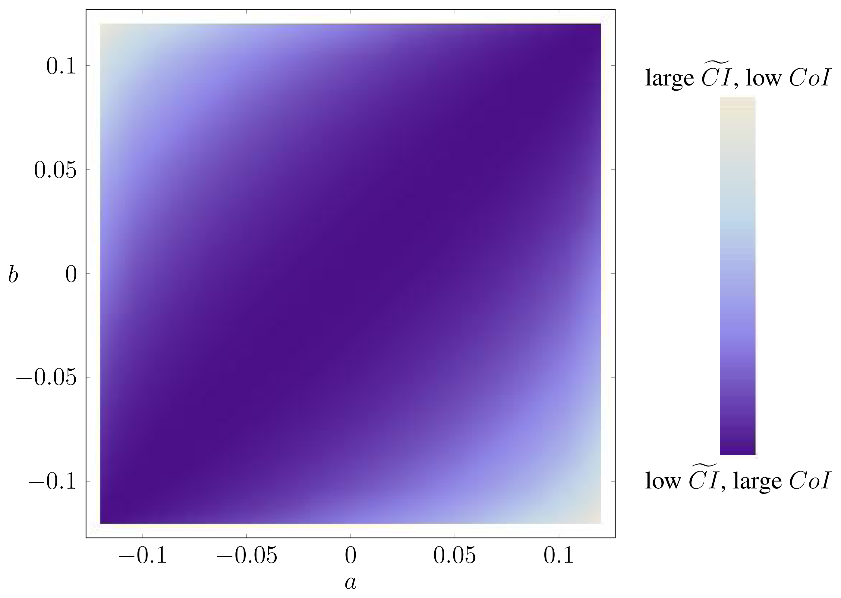
Example 31. The optimization problems in Lemma 4 can be very ill-conditioned, in the sense that there are directions in which the function varies fast and other directions in which the function varies slowly. As an example, let P be the distribution of three i.i.d. uniform binary random variables. In this case, ΔP is a square. Figure A.1 contains a heat map of CoIQ on ΔP, where ΔP is parametrized by:
Clearly, the function varies very little along one of the diagonals. In fact, along this diagonal, X is independent of (Y, Z), corresponding to a very low synergy.
Although, in this case, the optimizing probability distribution is unique, it can be difficult to find. For example, Mathematica’s function FindMinimum does not always find the true optimum out of the box (apparently, FindMinimum cannot make use of the convex structure in the presence of constraints) [12].

A.3. Technical Proofs
Proof of Lemma 9
Since , if , then:
To show that MIQ0 (Y : Z) = 0 is also sufficient, observe that:
by construction of Q0, and that:
by the assumption that MIQ0 (Y : Z) = 0. Therefore, by Lemma 29, all partial derivatives vanish at Q0. Hence, Q0 solves the optimization problems in Lemma 4, and .
Proof of Lemma 19
Let Q1 and Q2 be solutions of the optimization problems from Lemma 4 for (X1, Y1, Z1) and (X2, Y2, Z2) in the place of (X, Y, Z), respectively. Consider the probability distribution Q defined by:
Since (X1, Y1, Z1) is independent of (X2, Y2, Z2) (under P), Q ∈ ΔP. We show that Q solves the optimization problems from Lemma 4 for X = (X1, X2), Y = (Y1, Y2) and Z = (Z1, Z2). We use the notation from Appendices A.1 and A.2.
If , then:
Therefore, by Lemma 29,
and hence, again by Lemma 29, Q is a critical point and solves the optimization problems.
Proof of Lemma 21
We use the notation from [6]. The information divergence is jointly convex. Therefore, any critical point of the divergence restricted to a convex set is a global minimizer. Let y ∈
. Then, it suffices to show: If P satisfies the two conditional independence statements, then the marginal distribution PX of X is a critical point of D(P(·|y)||Q) for Q restricted to Ccl(〈Z〉X); for if this statement is true, then Py↘Z = PX; thus
, and finally, Ired(X : Y ; Z) = 0.
Let z, z′ ∈
. The derivative of D(P(·|y)||Q) at Q = PX in the direction P(X|z) − P(X|z′) is:
Now, Y ⫫ Z |X implies:
and Y ⫫ Z implies P(y)P(z) = P(y, z) and P(y)P(z′) = P(y, z′). Together, this shows that PX is a critical point.
Conflicts of Interest
The authors declare no conflict of interest.
- Author’s ContributionAll authors contributed to the design of the research. The research was carried out by all authors, with main contributions by Bertschinger and Rauh. The manuscript was written by Rauh, Bertschinger and Olbrich. All authors read and approved the final manuscript.
References
- McGill, W.J. Multivariate information transmission. Psychometrika 1954, 19, 97–116. [Google Scholar]
- Schneidman, E.; Bialek, W.; Berry, M.J.I. Synergy, redundancy, and independence in population codes. J. Neurosci 2003, 23, 11539–11553. [Google Scholar]
- Latham, P.E.; Nirenberg, S. Synergy, redundancy, and independence in population codes, revisited. J. Neurosci 2005, 25, 5195–5206. [Google Scholar]
- Williams, P.; Beer, R. Nonnegative decomposition of multivariate information. arXiv:1004.2515v1. 2010. [Google Scholar]
- Griffith, V.; Koch, C. Quantifying synergistic mutual information. arXiv:1205.4265. 2013. [Google Scholar]
- Harder, M.; Salge, C.; Polani, D. Bivariate measure of redundant information. Phys. Rev. E 2013, 87, 012130. [Google Scholar]
- Bertschinger, N.; Rauh, J.; Olbrich, E.; Jost, J. Shared information–new insights and problems in decomposing Information in Complex Systems. Proceedings of the ECCS 2012, Brussels, September 3–7 2012; pp. 251–269.
- Bertschinger, N.; Rauh, J. The blackwell relation defines no lattice. arXiv:1401.3146. 2014. [Google Scholar]
- Blackwell, D. Equivalent comparisons of experiments. Ann. Math. Stat 1953, 24, 265–272. [Google Scholar]
- Rauh, J.; Bertschinger, N.; Olbrich, E.; Jost, J. Reconsidering unique information: Towards a multivariate information Decomposition. arXiv:1404.3146. 2014. Accepted for ISIT 2014. [Google Scholar]
- Hoşten, S.; Sullivant, S. Gröbner bases and polyhedral geometry of reducible and cyclic Models. J. Combin. Theor. A 2002, 100, 277–301. [Google Scholar]
- Wolfram Research, Inc, Mathematica, 8th ed; Wolfram Research Inc: Champaign, Illinois, USA, 2003.

| Example | Imin | Note | ||
|---|---|---|---|---|
| Rdn | 0 | 1 | 1 | X = Y = Z uniformly distributed |
| Unq | 1 | 0 | 1 | X = (Y, Z), Y, Z i.i.d. |
| Xor | 1 | 0 | 0 | X = Y XORZ, Y, Z i.i.d. |
| And | 1/2 | 0.311 | 0.311 | X = Y AND Z, Y, Z i.i.d. |
| RdnXor | 1 | 1 | 1 | X = (Y1 XOR Z1, W), Y = (Y1, W), Z = (Z1, W), Y1, Z1, W i.i.d. |
| RdnUnqXor | 1 | 1 | 2 | X = (Y1 XOR Z1, (Y2, Z2), W), Y = (Y1, Y2, W), Z = (Z1, Z2, W), Y1, Y2, Z1, Z2, W i.i.d. |
| XorAnd | 1 | 1/2 | 1/2 | X = (Y XORZ, Y AND Z), Y, Z i.i.d. |
| Copy | 0 | MI(X : Y ) | 1 | X = (Y, Z) |
© 2014 by the authors; licensee MDPI, Basel, Switzerland This article is an open access article distributed under the terms and conditions of the Creative Commons Attribution license (http://creativecommons.org/licenses/by/3.0/).
Share and Cite
Bertschinger, N.; Rauh, J.; Olbrich, E.; Jost, J.; Ay, N. Quantifying Unique Information. Entropy 2014, 16, 2161-2183. https://doi.org/10.3390/e16042161
Bertschinger N, Rauh J, Olbrich E, Jost J, Ay N. Quantifying Unique Information. Entropy. 2014; 16(4):2161-2183. https://doi.org/10.3390/e16042161
Chicago/Turabian StyleBertschinger, Nils, Johannes Rauh, Eckehard Olbrich, Jürgen Jost, and Nihat Ay. 2014. "Quantifying Unique Information" Entropy 16, no. 4: 2161-2183. https://doi.org/10.3390/e16042161