Identifying the Coupling Structure in Complex Systems through the Optimal Causation Entropy Principle

Abstract

Inferring the coupling structure of complex systems from time series data in general by means of statistical and information-theoretic techniques is a challenging problem in applied science. The reliability of statistical inferences requires the construction of suitable information-theoretic measures that take into account both direct and indirect influences, manifest in the form of information flows, between the components within the system. In this work, we present an application of the optimal causation entropy (oCSE) principle to identify the coupling structure of a synthetic biological system, the repressilator. Specifically, when the system reaches an equilibrium state, we use a stochastic perturbation approach to extract time series data that approximate a linear stochastic process. Then, we present and jointly apply the aggregative discovery and progressive removal algorithms based on the oCSE principle to infer the coupling structure of the system from the measured data. Finally, we show that the success rate of our coupling inferences not only improves with the amount of available data, but it also increases with a higher frequency of sampling and is especially immune to false positives.

1. Introduction

Deducing equations of dynamics from empirical observations is fundamental in science. In real-world experiments, we gather data of the state of a system. Then, to achieve the comprehension of the mechanisms behind the system dynamics, we often need to reconstruct the underlying dynamical equations from the measured data. For example, the laws of celestial mechanics were deduced based on observations of planet trajectories [1]; the forms of chemical equations were inferred upon empirical reaction relations and kinetics [2]; the principles of economics were uncovered through market data analysis [3]. Despite such important accomplishments, the general problem of identifying dynamical equations from data is a challenging one. Early efforts, such as the one presented in [4], utilized embedding theory and relative entropy to reconstruct the deterministic component of a low-dimensional dynamical system.

Later, more systematic methods were developed to design optimal models from a set of basis functions, where model quality was quantified in various ways, such as the Euclidean norm of the error [5], the length of the prediction time window (chaotic shadowing) [6] or the sparsity in the model terms (compressive sensing) [7]. Each method achieved success in a range of systems, but none is generally applicable. This is, in fact, not surprising in light of the recent work that showed that the identification of exact dynamical equations from data is NP hard and, therefore, unlikely to be solved efficiently [8].

Fortunately, in many applications, the problem we face is not necessarily the extraction of exact equations, but rather, uncovering the cause-and-effect relationships (i.e., direct coupling structure) among the components within a complex system. For example, in medical diagnosis, the primary goal is to identify the causes of a disease and/or the roots of a disorder, so as to prescribe effective treatments. In structural health monitoring, the main objective is to locate the defects that could cause abrupt changes of the connectivity structure and adverse the performance of the system. Due to its wide range of applications, the problem of inferring causal relationships from observational data has attracted broad attention over the past few decades [9–25].

Among the various notions of causality, we adopt the one originally proposed by Granger, which relies on two basic principles [10,11]:

(1)

The cause should occur before the effect (caused);

(2)

The causal process should carry information (unavailable in other processes) about the effect.

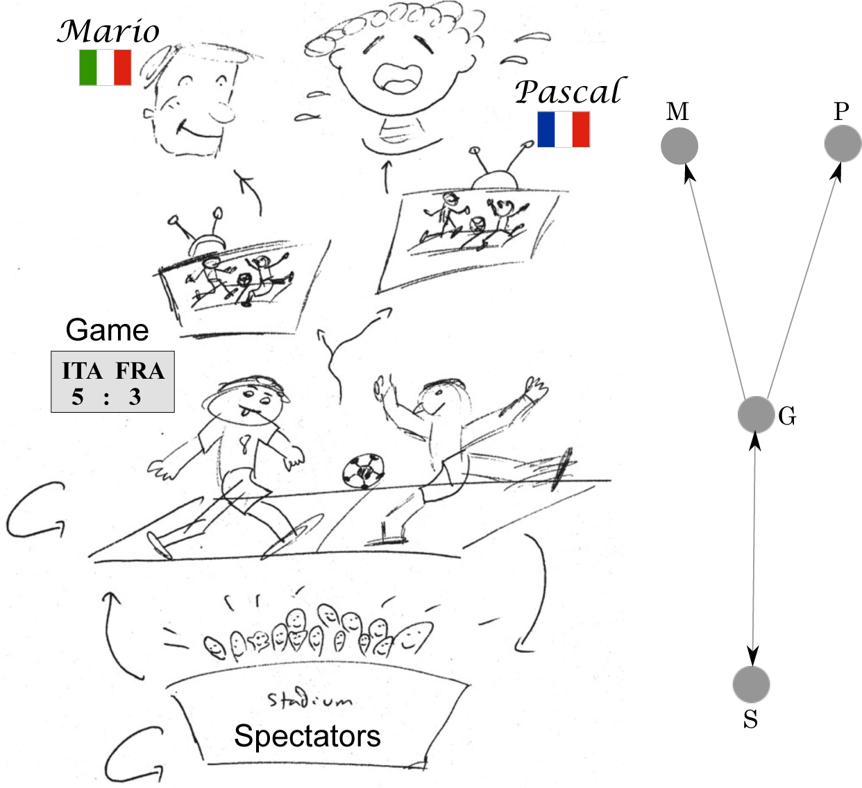
A causal relationship needs to satisfy both requirements. See Figure 1 as a schematic illustration.

The classical Granger causality is limited to coupled linear systems, while most recently developed methods based on information-theoretic measures are applicable to virtually any model, although their effectiveness relies on the abundance of data. Notably, transfer entropy (TE), a particular type of conditional mutual information, was introduced to quantify the (asymmetric) information flow between pairs of components within a system [26,27] and further developed to detect the directionality of coupling in systems with two components [28–30]. The application of these pairwise inference methods to identify direct coupling in systems with more than two components warrants caution: the inferred couplings are often incorrect regardless of the amount of available data [24,25,31]. In fact, Granger’s second principle implies that a true causal relationship should remain effective upon the removal of all other possible causes. As a consequence, an inference method cannot correctly identify the direct coupling between two components in a system without appropriate conditioning on the remaining components [15,24,25].

Inferring causal relationships in large-scale complex systems is challenging. For a candidate causal relationship, one needs to effectively determine whether the cause and effect is real or is due to the presence of other variables in the system. A common approach is to test the relative independence between the potential cause and effect conditioned on all other variables, as demonstrated in linear models [17,33,34]. Although analytically rigorous, this approach requires the estimation of the related inference measures for high dimensional random variables from (often limited available) data, and therefore, suffers the curse of dimensionality [22]. Many heuristic alternatives have been proposed to address this issue. The essence of these alternative approaches is to repeatedly measure the relative independence between the cause and effect conditioned on a combination of the other variables, often starting with subsets of only a few variables [22,23,35]. As soon as one such combination renders the proposed cause and effect independent, the proposed relationship is rejected, and there is no need to condition on subsets with more variables. The advantage of such an approach is that it reduces the dimensionality of the sample space if the proposed relationship is rejected at some point. However, if the relationship is not rejected, then the algorithm will continue, potentially having to enumerate over all subsets of the other variables. In this scenario, regardless of the dimensionality of the sample space, the combinatorial search itself is often computationally infeasible for large or even moderate-size systems.

In our recent work in [24,25], we introduced the concept of causation entropy (CSE), proposed and proved the optimal causation entropy (oCSE) principle and presented efficient algorithms to infer causal relationships within large complex systems. In particular, we showed in [25] that by a combination of the aggregate discovery and progressive removal of variables, all causal relationships can be correctly inferred in an computational feasible and data-efficient manner. We repeat for emphasis that without properly accounting for multiple interactions and conditioning accordingly, erroneous or irrelevant casual influences may be inferred, and specifically, any pairwise-only method will inherent the problem that many false-positive connections will arise. The design of oCSE specifically addresses this issue.

In this paper, we focus on the problem of inferring the coupling structure in synthetic biological systems. When the system reaches an equilibrium state, we employ random perturbations to extract time series that approximate a linear Gaussian stochastic process. Then, we apply the oCSE principle to infer the system’s coupling structure from the measured data. Finally, we show that the success rate of causal inferences not only improves with the amount of available data, but it also increases with the higher frequency of sampling.

2. Inference of Direct Coupling Structure through Optimal Causation Entropy

To infer causal structures in complex systems, we clearly need to specify the mathematical assumptions under which the task is to be accomplished. Accurate mathematical modeling of complex systems demands taking into account the coupling of neglected degrees of freedom or, more generally, the fluctuations of external fields that describe the environment interacting with the system itself [36]. This requirement can be addressed in a phenomenological manner by adding noise in deterministic dynamical models. The addition of noise, in turn, generally leads to the stochastic process formalism used in the modeling of natural phenomena [37]. We study the system in a probabilistic framework. Suppose that the system contains n components, V = {1, 2,…, n}. Each component i is assumed to be influenced by a unique set of components, denoted by N_i. Let:

$$X_t=[X_t^{(1)},X_t^{(2)},\dots ,X_t^{(n)}]$$

(1)

be a random variable that describes the state of the system at time t. For a subset K = {k₁, k₂,…., k_q} ⊂ V, we define:

$$X_t^{(K)}\equiv \left[X_t^{(k_1)},X_t^{(k_2)},\dots ,X_t^{(k_q)}\right].$$

(2)

2.1. Markov Conditions

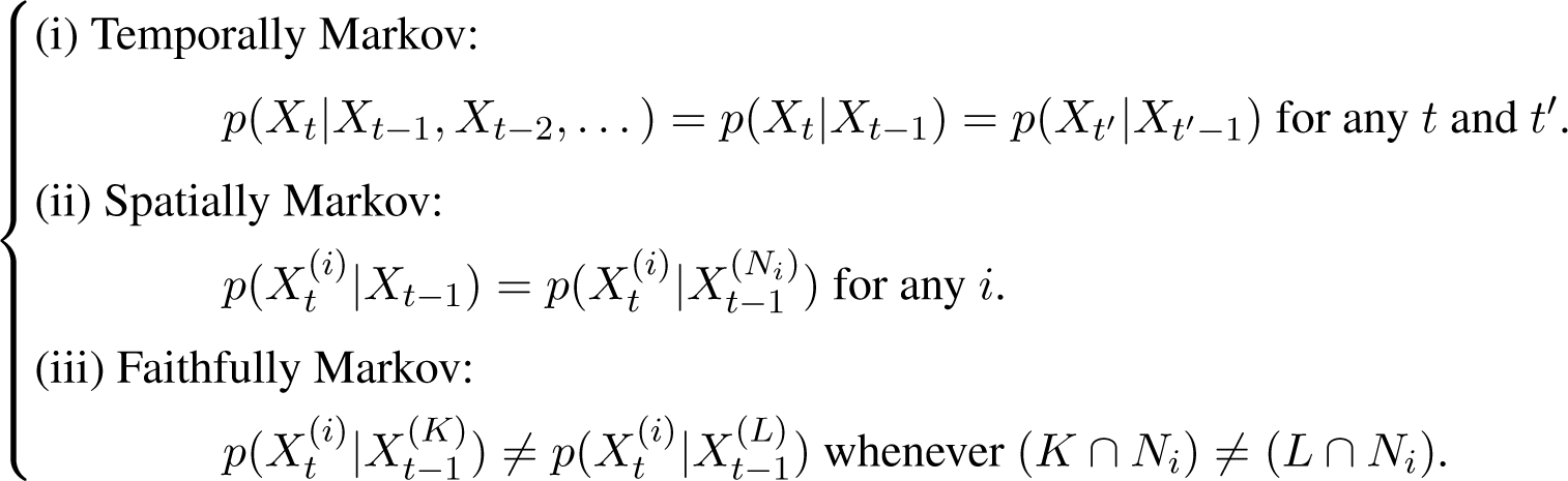
We assume that the system undergoes a stochastic process with the following Markov conditions [25].

(3)

Here, p(·|·) denotes conditional probability. The relationship between two probability density functions p₁ and p₂ is denoted as “p₁ = p₂” iff they equal almost everywhere, and “p₁ ≠ p₂” iff there is a set of positive measure on which the two functions do not equal. Note that the Markov conditions stated in Equation (3) ensure that for each component i, there is a unique set of components N_i that renders the rest of the system irrelevant in making inference about X⁽ⁱ⁾ and each individual component in N_i presents an observable cause regardless of the presence or absence of the other components.

Although several complex systems can be properly modeled in terms of Markov processes [38], we cannot avoid recalling that, after all, non-Markov is the rule and Markov is only the exception in nature [39]. Therefore, it is important to develop a theoretical framework suitable for identifying coupling structures in complex systems driven by correlated fluctuations where memory effects cannot be neglected. It is in fact possible to relax the assumptions in Equation (3) to a stochastic process with finite or vanishing memory, as discussed in the last section of the paper.

The problem of inferring direct (or causal) couplings can be stated as follows. Given time series data $\left\{x_t^{(i)}\right\}(i=1,2,\dots ,n;t=1,2,\dots T)$ drawn from a stochastic process that fulfills the Markov conditions in Equation (3), the goal is to uncover the set of causal components N_i for each i. We solve this problem by means of algorithms that implement the oCSE principle.

2.2. Causation Entropy

We follow Shannon’s definition of entropy to quantify the uncertainty of a random variable. In particular, the entropy of a continuous random variable X is defined as [40]:

$$h\left(X\right)\equiv -{\displaystyle \int p\left(x\right)\log p\left(x\right)dx,}$$

(4)

where p(x) is the probability density function of X. The conditional entropy of X given Y is defined as [41]:

$$h\left(X|Y\right)\equiv -{\displaystyle \int p\left(x,y\right)\log p\left(x|y\right)dxdy.}$$

(5)

Equations (4) and (5) are valid for both univariate and multivariate random variables. Consider a stochastic process. Let I, J and K be arbitrary sets of components within the system. We propose to quantify the influence of J on I conditioned upon K via the CSE:

$$C_{J\to I|K}=\underset{t\to \infty }{\lim }[h(X_{t+1}^{(I)}|X_t^{(K)})-h(X_{t+1}^{(I)}|X_t^{(K)},X_t^{(J)})],$$

(6)

provided that the limit exists [24,25]. Since, in general, H(X|Y)−H(X|Y, Z) = I(X; Z|Y), where the latter defines the conditional mutual information between X and Z conditioned on Y, it follows from the nonnegativity of conditional mutual information that CSE is nonnegative. When K = Ø, we omit the conditioning part and simply use the notation C_J→I. Notice that if K = I, CSE reduces to TE. On the other hand, CSE generalizes TE by allowing K to be an arbitrary set of components.

2.3. Optimal Causation Entropy Principle

In our recent work [25], we revealed the equivalence between the problem of identifying the causal components and the optimization of CSE. In particular, we proved that for an arbitrary component i, its unique set of causal components N_i is the minimal set of components that maximizes CSE. Given the collection of sets (of components) with maximal CSE with respect to component i,

$${\mathcal{K}}_i=\{K\subset \mathcal{V}|C_{K\to i}\ge C_{K^{\prime }\to i}\text{for any }{K}^{\prime }\subset \mathcal{V}\},$$

(7)

it was shown that N_i is the unique set in ${\mathcal{K}}_i$ with minimal cardinality, i.e.,

$$N_i={\cap }_{K\in {\mathcal{K}}_i}K={\text{argmin}}_{K\in {\mathcal{K}}_i}\left|K\right|.$$

(8)

We refer to this minimax principle as the oCSE principle [25].

2.4. Computational Causality Inference

Based on the oCSE principle, we developed two algorithms whose joint sequential application allows the inference of causal relationships within a system [25]. The goal of these algorithms is to effectively and efficiently identify for a given component i the direct causal set of components N_i. The first algorithm aggregatively identifies the potential causal components of i. The outcome is a set of components M_i that includes N_i as its subset, with possibly additional components. These additional components are then progressively removed by applying the second algorithm.

For a given component i, the first algorithm, referred to as aggregative discovery, starts by selecting a component k₁ that maximizes CSE, i.e.,

$$k_1={\mathrm{argmax}}_{k\in \mathcal{V}}{C}_{k\to i}.$$

(9)

Then, at each step j (j = 1, 2,…), a new component k_j+1 is identified among the rest of the components to maximize the CSE conditioned on the previously selected components:

$$k_{j+1}=\underset{k\in v/\{k_1,k_2,\dots ,k_j\}}{\mathrm{argmax}}{C}_{k\to i\left|\right\{k_1,k_2,\dots ,k_j\}}.$$

(10)

Recall that CSE is nonnegative. The above iterative process is terminated when the corresponding maximum CSE equals zero, i.e., when:

$$\underset{k\in \mathcal{V}/\{k_1,k_2,\dots k_j\}}{max}{C}_{k\to i\left|\right\{k_1,k_2,\dots k_j\}}=0,$$

(11)

and the outcome is the set of components M_i = {k₁, k₂,…, k_j} ⊃ N_i.

Next, to remove non-causal components (including indirect and spurious ones) that are in M_i, but not in N_i, we employ the second algorithm, referred to as progressive removal. A component k_j in M_i is removed when:

$$C_{k_j\to i\left|M_i\text{/}\right\{k_j\}}=0,$$

(12)

and M_i is updated accordingly (An alternative way of removing non-causal components is to test conditioning on subsets of M_i with increasing cardinality, potentially reducing the dimensionality of sample space at the expense of increased computational burden. This is similar to the PC-algorithm originally proposed in Reference [12] and successfully employed in Reference [22], with the key difference that here the enumeration of conditioning subsets only needs to be performed for M_i instead of for the entire system V). After removing all such components, the resulting set is identified as N_i.

2.5. Estimation of CSE in Practice

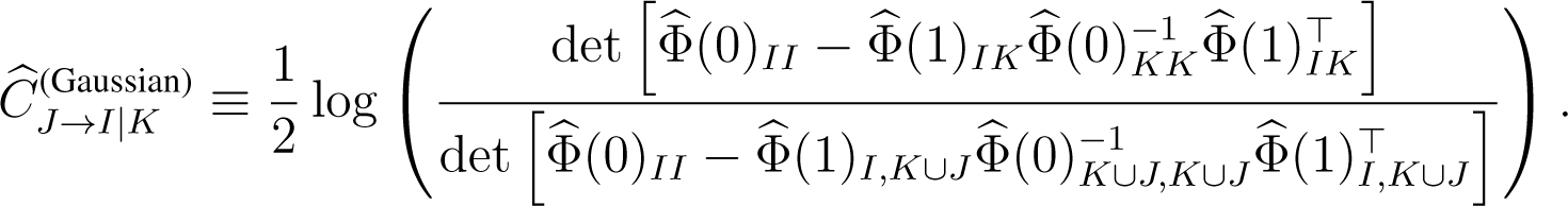
In practice, causation entropy C_J→I|K needs to be estimated from data. We define the Gaussian estimator of causation entropy as:

(13)

Here:

$$\Phi {(\tau )}_{IJ}\equiv \text{Cov}+(X_{t+\tau }^{(I)},X_t^{(J)})$$

(14)

denotes a covariance matrix where τ ∈ {0, 1}, and $\widehat{\Phi }{\left(\tau \right)}_{IJ}$ denotes the corresponding sample covariance matrix estimated from the data [25]. The estimation ${\widehat{C}}_{J\to I|K}^{(\text{Gaussian})}\approx C_{J\to I|K}$ if: (i) the underlying random variables are Gaussians; and (ii) the amount of data is sufficient for the relevant sample covariances to be close to their true values. When the underlying random variables are non-Gaussian, an efficient estimator for CSE is yet to be fully developed. As previously pointed out, binning-related estimators, although conceptually simple, are generally inefficient, unless the sample space is low-dimensional [16]. To gain efficiency and to minimize bias for a large system where the sample space is high-dimensional, an idea would be to build upon the k-nearest neighbor estimators of entropic measures [29,42–44].

Regardless of the method that is being adopted for the estimation of C_J→I|K, the estimated value is unlikely to be exactly zero due to limited data and numerical precision. In practice, it is necessary to decide whether or not the estimated quantity should be regarded as zero. Such a decision impacts the termination criterion Equation (11) in the aggregative discovery algorithm and determines which components need to be removed based on Equation (12) in the progressive removal algorithm. As discussed in [25], such a decision problem can be addressed via a nonparametric statistical test, called the permutation test, as described below.

For given time series data $\left\{x_t^{(i)}\right\}(i=1,2,\dots ,n;t=1,2,\dots ,T)$, let ${\widehat{C}}_{J\to I|K}$ denote the estimated value of C_J→I|K. Based on the set of components J and a permutation function π on the set of integers from one to T, the corresponding permuted time series $\left\{y_t^{(i)}\right\}$ is defined as:

$$y_t^{(i)}=\{\begin{array}{cc}{x}_{\pi (t)}^{(i)}& \text{if }i\in J,\\ x_t^{(i)}& \text{if }i\notin J.\end{array}$$

(15)

To apply the permutation test, we generate a number of randomly permuted time series (the number will be denoted by r). We then compute the causation entropy from J to I conditioned on K for each permuted time series to obtain r values of the estimates, which are consequently used to construct an empirical cumulative distribution F as:

$$F(C)\equiv \frac{1}{r}\left|\{{\widehat{C}}_{J\to I|K}^{(s)}:{\widehat{C}}_{J\to I|K}^{(s)}\le C,1\le s\le r\}\right|,$$

(16)

where ${\widehat{C}}_{J\to I|K}^{(s)}$ are estimates from the permuted time series with 1 ≤ s ≤ r and |·| denotes the cardinality of a set. Finally, with the null hypothesis that C_J→I|K = 0, we regard C_J→I|K as strictly positive if and only if:

$$F({\widehat{C}}_{J\to I|K})>\theta ,$$

(17)

where 0 < (1 − θ) < 1 is the prescribed significance level. In other words, the null hypothesis is rejected at level (1 − θ) if the above inequality holds. Therefore, the permutation test relies on two input parameters: (i) the number of random permutations r; and (ii) the significance level (1 − θ). In practice, the increase of r improves the accuracy of the empirical distribution at the expense of additional computational cost. A reasonable balance is often achieved when 10³ ≲ r ≲ 10⁴ [25]. The value of θ sets a lower bound on the false positive ratio and should be chosen to be close to one (for example, θ = 99%) [25].

3. Extracting Stochastic Time Series from Deterministic Orbits

Biological systems can exhibit both regular and chaotic features [45]. For instance, a healthy cardiac rhythm is characterized by a chaotic time series, whereas a pathological rhythm often exhibits regular dynamics [46]. Therefore, a decrease of the chaoticity of the cardiac rhythm is an alarming clinical signature. A similar connection between the regularity of the time series and pathology is observed in spontaneous neuronal bursting in the brain [47,48]. When a system settles into a periodic or equilibrium state, it becomes nearly impossible to infer the coupling structure among the variables, as the system is not generating any information to be utilized for inference. To overcome this difficulty, we propose to apply small stochastic perturbations to the system while in an equilibrium state (this is equivalent to adding dynamic noise to a system to facilitate coupling inference, as shown in [49]). Then, we measure the system’s response over short time intervals. Finally, we follow the oCSE principle and apply the aggregative discovery and progressive removal algorithms to the measured data to infer the couplings among the variables.

3.1. Dynamical System and Equilibrium States

Consider a continuous dynamical system:

$$dx/dt=f(x),$$

(18)

where $x={[x_1,x_2,\dots x_n]}^{\top }\in {\mathrm{ℝ}}^n$ is the n-dimensional state variable, the symbol “⊤” denotes transpose, and f = [f₁, f₂,…, f_n]^⊤: ℝⁿ → ℝⁿ is a smooth vector field, which models the dynamic rules of the system. A trajectory of the system (18) is a solution x(t) to the differential equation, Equation (18), with a given initial condition x(0) = x₀.

An equilibrium of the system is a state x^∗, such that f(x^∗) = 0. When a system reaches an equilibrium, the time evolution of the state ceases. An equilibrium x^∗ is called stable if nearby trajectories approach x^∗ forward in time, i.e., there exists a constant ρ > 0, such that $x(t)\stackrel{t\to \infty }{\to }x*$ whenever ‖x₀ – x*‖ < ρ, where ‖ · ‖ denotes the standard Euclidean norm. Otherwise, the equilibrium is called unstable.

3.2. Response of the System to Stochastic Perturbations

To gain information about the coupling structure of a system, it is necessary to apply external perturbations to “knock” the system out of an equilibrium state and observe how it responds to these perturbations. Suppose that we apply and record a sequence of random perturbations to the system in such a manner that before each perturbation, the system is given sufficient time to evolve back to its stable equilibrium. In addition, the response of the system is measured shortly after each perturbation, but before the system reaches the equilibrium again. Denote the stable equilibrium of interest as x^∗; we propose to repeatedly apply the following steps.

Step 1.

Allow the system to (spontaneously) reach x^∗.

Step 2.

At time t, apply and record a random perturbation ξ to the system, i.e., x(t) = x^∗ + ξ.

Step 3.

At time t + Δt, measure the rate of response, defined as η = [x(t + Δt) − x^∗ − ξ]/Δt.

Repeated application of these steps L times results in a collection of perturbations, denoted as $\left\{{\xi }_{\ell }\right\}$, and rates of response, denoted as {η_ℓ}, where ℓ = 1, 2,…, L. Here, each perturbation ξ_ℓ is assumed to be drawn independently from the same multivariate Gaussian distribution with zero mean and covariance matrix σ²$\mathbb{I}$. For a given equilibrium x^∗, in addition to L—the number of times the perturbations are applied—there are two more parameters in the stochastic perturbation process: the sample frequency defined as 1/Δt and the variance of perturbation defined as σ². To ensure that the perturbation approximates the linearized dynamics of the system, we require that 1/Δt ≫ 1 and σ ≪ 1. The influence of these parameters will be studied in the next section with a concrete example.

We remark here that the choice of Gaussian distribution is a practical rather than a conceptual one. In theory, any multivariate distribution can be used to generate the perturbation vector ξ_ℓ as long as the component-wise distributions of ${\xi }_{\ell }^{(i)}$ and ${\xi }_k^{(j)}$ are identical and independent whenever i ≠ j or ℓ ≠ k. In practice, since the effectiveness of any information theoretic method (including the one proposed here) depends on the estimation of entropies, choosing the perturbations to be Gaussian greatly improves the reliability of estimation and, thus, the accuracy of the inference. This is because the entropy of Gaussian variables depends only on covariances, rendering its estimation relatively straightforward [25,50,51].

Note that each perturbation ξ_ℓ and its response η_ℓ are related through the underlying nonlinear differential equation dx/dt = f (x), where the nonlinearity is encoded in the function f (x), which is assumed to be unknown. For an equilibrium x^∗, the dynamics of nearby trajectories can be approximated by its linearized system, as follows. Consider a state x ≈ x^∗ and define the new variable δx = x − x^∗. To the first order, the time evolution of δx can be approximated by the following linear system:

$$d(\delta x)/dt=Df(x*)\delta x,$$

(19)

where Df(·) is the n-by-n Jacobian matrix of f, defined as [D f (x)]_ij = ∂f_i/∂x_j. A sufficient condition for x^∗ to be stable is that all eigenvalues of Df(x^∗) must have negative real parts. From Equation (19), with the additional assumption that Δt ≪ 1, the relationship between the perturbation and response is approximated by the following equation:

$${\eta }_{\ell }=Df(x*){\xi }_{\ell }.$$

(20)

Note that since ξ_ℓ is a multivariate normal random variable and Df(x^∗) is a constant matrix, the variable η_ℓ is also (approximately) a multivariate normal random variable. Equation (20) therefore represents a drive-response type of Gaussian process.

4. Application to Synthetic Biology

4.1. The Repressilator

Cellular dynamics is centrally important in biology [52]. To describe and, to a certain extent, to understand what happens in cells, fluctuating chemical concentrations and reaction rates need to be measured experimentally. However, constructing dynamic models that accurately reproduce the observed phenomena in cells is quite challenging. An alternative approach consists in engineering synthetic biological systems that follow prescribed dynamic rules. An important example is the so-called repressilator (or repression-driven oscillator) presented in [53]. The repressilator is based upon three transcriptional repressors inserted into the E. coli bacteria with a plasmid. The three repressors, lacl, tetR and cl, are related as follows: lacl inhibits the transcription of the gene coding for tetR; tetR inhibits the transcription of the gene coding for cl; cl inhibits the transcription of the gene coding for lacl. In the absence of inhibition, each of the three proteins reaches a steady-state concentration resulting from a balance between its production and degradation rates within the bacterium. In the presence of cross-inhibition by the other two repressors, this network architecture potentially allows oscillations and other interesting dynamical behaviors and serves as a prototype of modeling the quorum sensing among bacteria species [54].

The repressilator dynamics can be modeled by a system of coupled differential equations, which describe the rates of change for the concentration p_i of each protein repressor and the concentration m_i of its associated mRNA in their network, as: [53]

(21)

where m₁ (p₁), m₂ (p₂) and m₃ (p₃) represent the mRNA (protein) concentration of the genes lacl, tetR and cl, respectively. See Figure 2a for a schematic representation of the system. Each ODE in Equation (21) consists of positive terms modeling the production rate and a negative term representing degradation. There are four parameters in the ODEs in Equation (21), namely: β is the ratio of the decay rate to the mRNA decay rate; n is the so-called Hill coefficient and describes the cooperativity of the binding of repressor to promoter; α₀, the leakiness of the promoter, is the rate of transcription of mRNA in the presence of saturating concentration of the repressor; α₀ + α is the additional rate transcription of mRNA in the absence of the inhibitor. Note that units of time and concentration Equation (21) have been rescaled in order to make these equations non-dimensional [53].

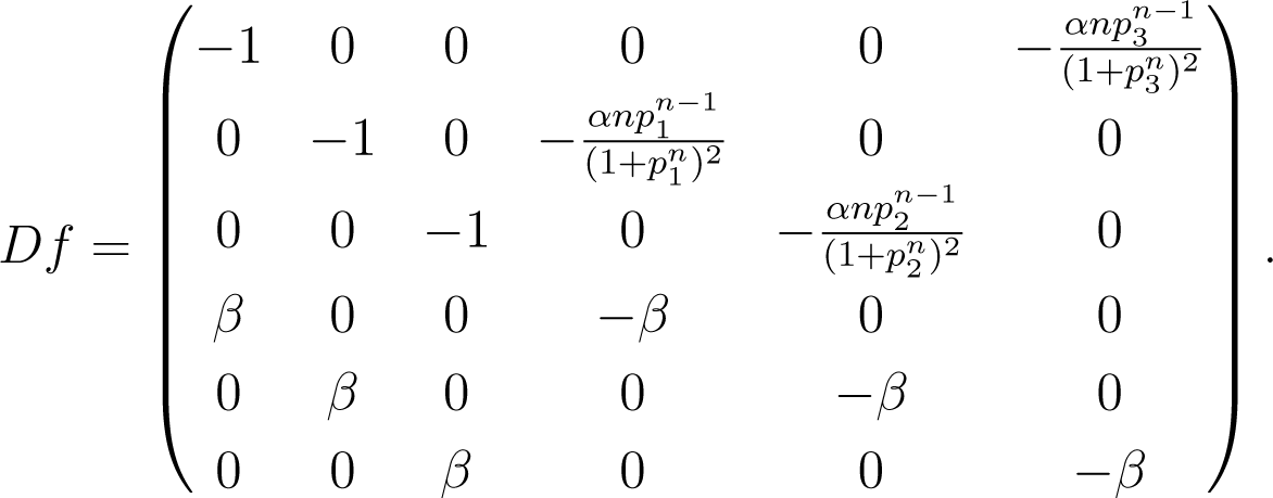
As shown in [53], there is an extended region in the parameter space for which the system described in Equation (21) exhibits a single stable equilibrium. The Jacobian matrix at the equilibrium is:

(22)

Problem statement: The goal of coupling inference is to identify the location of the nonzero entries of the Jacobian through time series generated by the system near equilibrium.

4.2. Inference of Coupling Structure via the Repressilator Dynamics

We consider the repressilator dynamics as modeled by Equation (21) with the parameters n = 2, α₀ = 0, α = 10 and β = 100. Under this setting, the system exhibits a single stable equilibrium [53] at which m₁ = m₂ = m₃ = p₁ = p₂ = p₃ = 2. Typical time series are shown in Figure 2b. After the system settles at the equilibrium, we apply the stochastic perturbations as described in Section 3 and obtain a time series of the perturbations {ξ_ℓ}, as well as responses {η_ℓ}. The goal is to identify, for each component (the mRNA or protein of a gene) in the system, the set of components that determine its dynamics (i.e., the variables that appear on the right-hand side of each relation in Equation (21)).

To apply our algorithms according to the oCSE principle, we define the set of random variables $X_t^{\left(i\right)}\left(i=1,2,\dots ,12;t=1,2,\dots \right)$ as:

$$X_t^{\left(i\right)}=\{\begin{array}{cc}{\xi }_t^{\left(i\right)}& \text{if}1\le i\le 6,\\ {\eta }_{t-1}^{\left(i-6\right)}& \text{if}7\le i\le 12.\end{array}$$

(23)

The approximate relationship between the perturbation and response as in 0Equation (20) can be expressed as:

$$X_{t+1}^{\left(I\right)}=A{X}_t^{\left(J\right)},$$

(24)

where I = {7, 8,…, 12}, J = {1, 2,…, 6} and A = Df(x^∗). Since this equation defines a stochastic process that satisfies the Markov assumptions in Equation (3), the oCSE principle applies. This implies that the direct couplings can be correctly inferred, at least in principle, by jointly applying the aggregative discovery and progressive removal algorithms.

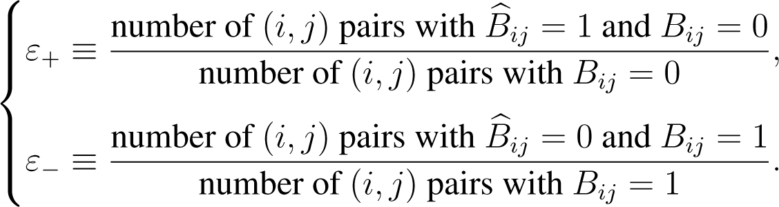
Since the perturbations {ξ_ℓ} and responses {η_ℓ} depend on the number of samples L, the rate of perturbation 1/∆t and the variance of perturbation σ², so is the accuracy of the inference. Next, we explore the change in performance of our approach by varying these parameters. We use two quantities to measure the accuracy of the inferred coupling structure, namely, the false positive ratio ε₊ and the false negative ratio ε₋. Since our goal is to infer the structure rather than the weights of the couplings, we focus on the structure of the Jacobian matrix Df(x^∗), encoded in the binary matrix B, where:

$${\left[B\right]}_{ij}=\{\begin{array}{cc}1,& \text{if}{\left[Df\left(x*\right)\right]}_{ij}\ne 0,\\ 0,& \text{otherwise}.\end{array}$$

(25)

On the other hand, applying the oCSE principle, the inferred direct coupling structure gives rise to the estimated binary matrix $\widehat{B}$ where:

$${\left[\widehat{B}\right]}_{ij}=\{\begin{array}{cc}1,& \text{if}j\text{is a direct causal component of}i,\\ 0,& \text{otherwise}.\end{array}$$

(26)

Given matrices B and $\widehat{B}$, the false positive and false negative ratios are defined, respectively, as:

(27)

It follows that 0 ≤ ε₊, ε₋ ≤ 1 and ε₊ = ε₋ = 0 when exact (error-free) inference is achieved.

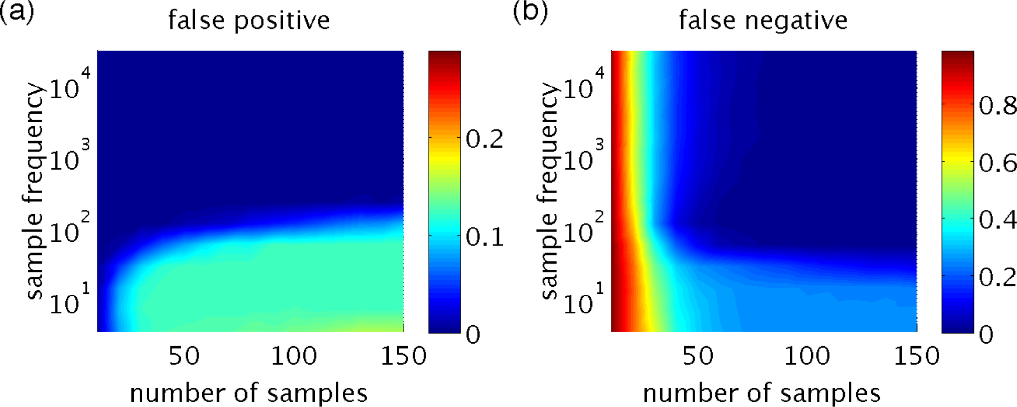
Figure 3a,b shows that both the false positives and false negatives converge as the number of samples increases. However, they converge to zero only if the rate of perturbation is sufficiently high. Figure 3c,d supports this observation and, in addition, shows that in the high rate of perturbation regime, exact inference is achieved with a sufficient number of samples (in this case, L ∼ 100). The combined effects of L and 1/∆t are shown in Figure 4. In all simulations, the variation of the perturbation is set to be σ² = 10⁻⁴ and is found to have little effect on the resulting inference, provided that it is sufficiently small to keep the linearization in Equations (20) and (24) valid.

5. Discussion and Conclusions

5.1. Results Summary

In this paper, we considered the challenging problem of inferring the causal structure of complex systems from limited available data (enjoy Figure 1 for a cartoon depiction of the concept of causality during a soccer game). Specifically, we presented an application of the so-called oCSE principle to identify the coupling structure of a synthetic biological system, the repressilator. First, we briefly reviewed the main points of the oCSE principle (Equations (7) and (8)), which states that for an arbitrary component i of a complex system, its unique set of causal components N_i is the minimal set of components that maximizes CSE (causation entropy, defined in Equation (6) is a generalization of transfer entropy). We strengthen in this work our claim that CSE is a suitable information-theoretic measure for reliable statistical inferences, since it takes into account both direct and indirect influences that appear in the form of information flows between nodes of networks underlying complex systems. We also devoted some attention to the implementation of the oCSE principle. This task is accomplished by means of the joint sequential application of two algorithms, aggregative discovery and progressive removal, respectively. Second, having introduced the main theoretical and computational frameworks, we used a stochastic perturbation approach to extract time series data approximating a Gaussian process when the model system—the repressilator (see Equation (21))—reaches an equilibrium configuration. We then applied the above-mentioned algorithms implementing the oCSE principle in order to infer the coupling structure of the model system from the observed data. Finally, we numerically showed that the success rate of our causal entropic inferences not only improves with the amount of available measured data (Figure 2a), but it also increases with a higher frequency of sampling (Figure 2b).

One especially important feature of our oCSE-based causality inference approach is that it is immune (in principle) to false positives. When data is sufficient, false positives are eliminated by sequential joint application of the aggregative discovery and progressive removal algorithms, as well as raising the threshold θ used in the permutation test (see [25] for a more detailed investigation of this point). In contrast, any pairwise causality measure without additional appropriate conditioning will in principle be susceptible to false positives, result in too many connections and, sometimes, even, implies that everything causes everything. Such a limitation is intrinsic and cannot be overcome merely by gathering more data [25]. On the other hand, false negatives are less common in practice and are usually caused by ineffective statistical estimation or insufficient data.

5.2. oCSE for General Stochastic Processes

We presented the oCSE principle for stochastic processes under the Markov assumptions stated in Equation (3). From an inference point of view, each and every one of these assumptions has a well-defined interpretation. For instance, the temporal Markov condition implies the stationarity of causal dependences between nodes. The loss of temporal stationarity could be addressed by partitioning the time series data into stationary segments and, then, performing time-dependent inferences. Clearly, such inferences would require extra care. Furthermore, the loss of the spatially and/or faithfully Markov condition would imply that the set of nodes that directly influence any given node of the network describing the complex system is no longer minimal and unique. Causality inference in this case becomes an ill-posed problem. These issues will be formally addressed in a forthcoming work.

Note that a finite k-th order Markov process {X_t} can always be converted into a first-order (memoryless) one {Z_t} by lifting, or in other words, defining new random variables Z_t = (X_t−k+1, X_t−k+2,…, X_t) [55]. In this regard, the oCSE principle extends naturally to an arbitrary finite-order Markov process. On the other hand, for a general stationary stochastic process that is not necessarily Markov (i.e., considering a process with potentially infinite memory), there might exist an infinite number of components from the past that causally influence the current state of a given component. However, under an assumption of vanishing (or fading) memory, such influences decay rapidly as a function of the time lag, and consequently, the process itself can be approximated by a finite-order Markov chain [56–59]. We plan to leave such generalizations for forthcoming investigations.

References

- Fitzpatrick, R. An Introduction to Celestial Mechanics; Cambridge University Press: New York, NY, USA, 2012. [Google Scholar]
- Atkins, P.; de Paula, J. Physical Chemistry, 9th ed.; W. H. Freeman Publishers: New York, NY, USA, 2010. [Google Scholar]
- Mankiw, N.G. Principles of Economics, 6th ed.; Cengage Learning: Stamford, CT, USA, 2011. [Google Scholar]
- Crutchfield, J.P.; McNamara, B.S. Equations of motions from a data series. Complex Syst 1987, 1, 417. [Google Scholar]
- Yao, C.; Bollt, E.M. Modeling and nonlinear parameter estimation with Kronecker product representation for coupled oscillators and spatiotemporal systems. Phys. Nonlinear Phenom 2007, 227, 78–99. [Google Scholar]
- Sun, J.; Bollt, E.M.; Nishikawa, T. Judging model reduction of complex systems. Phys. Rev. E 2011, 83, 046125. [Google Scholar]
- Wang, W.-X.; Yang, R.; Lai, Y.-C.; Kovanis, V.; Harrison, M.A.F. Time-series based prediction of complex oscillator networks via compressive sensing. Europhys. Lett 2011, 94, 48006. [Google Scholar]
- Cubitt, T.S.; Eisert, J.; Wolf, M.W. Extracting dynamical equations from experimental data is NP hard. Phys. Rev. Lett 2012, 108, 120503. [Google Scholar]
- Heider, F. Social perception and phenomenal causality. Psychol. Rev 1944, 51, 358–374. [Google Scholar]
- Granger, C.W.J. Investigating causal relations by econometric models and cross-spectral methods. Econometrica 1969, 37, 425–438. [Google Scholar]
- Granger, C.W.J. Some recent developments in a concept of causality. J. Econom 1988, 39, 199–211. [Google Scholar]
- Spirtes, P.; Glymour, C.N.; Scheines, R. Causation, Prediction, and Search, 2nd ed.; MIT Press: Cambridge, MA, USA, 2000. [Google Scholar]
- Rothman, K.J.; Greenland, S. Causation and causal inference in epidemiology. Am. J. Public Health 2005, 95, S144–S150. [Google Scholar]
- Caticha, A.; Cafaro, C. From information geometry to Newtonian dynamics, 8–13 July 2007; 954, pp. 165–174.
- Frenzel, S.; Pompe, B. Partial mutual information for coupling analysis of multivariate time series. Phys. Rev. Lett 2007, 99, 204101. [Google Scholar]
- Hlaváčková-Schindlera, K.; Paluš, M.; Vejmelka, M.; Bhattacharya, J. Causality detection based on information-theoretic approaches in time series analysis. Phys. Rep 2007, 441, 1–46. [Google Scholar]
- Guo, S.; Seth, A.K.; Kendrick, K.M.; Zhou, C.; Feng, J. Partial Granger causality—Eliminating exogenous inputs and latent variables. J. Neurosci. Methods 2008, 172, 79–93. [Google Scholar]
- Heckman, J.J. Econometric causality. Int. Stat. Rev 2008, 76, 1–27. [Google Scholar]
- Pearl, J. Causality: Models, Reasoning and Inference, 2nd ed.; Cambridge University Press: Cambridge, UK, 2009. [Google Scholar]
- Gao, Q.; Duan, X.; Chen, H. Evaluation of effective connectivity of motor areas during motor imagery and execution using conditional Granger causality. NeuroImage 2011, 54, 1280–1288. [Google Scholar]
- Vicente, R.; Wibral, M.; Lindner, M.; Pipa, G. Transfer entropy—A model-free measure of effective connectivity for the neurosciences. J. Comput. Neurosci 2011, 30, 45–67. [Google Scholar]
- Runge, J.; Heitzig, J.; Petoukhov, V.; Kurths, J. Escaping the curse of dimensionality in estimating multivariate transfer entropy. Phys. Rev. Lett 2012, 108, 258701. [Google Scholar]
- Runge, J.; Heitzig, J.; Marwan, N.; Kurths, J. Quantifying causal coupling strength: A lag-specific measure for multivariate time series related to transfer entropy. Phys. Rev. E 2012, 86, 061121. [Google Scholar]
- Sun, J.; Bollt, E.M. Causation entropy identifies indirect influences, dominance of neighbors and anticipatory couplings. Phys. Nonlinear Phenom 2014, 267, 49–57. [Google Scholar]
- Sun, J.; Taylor, D.; Bollt, E.M. Causal network inference by optimal causation entropy 2014, arXiv, 1401.7574.
- Schreiber, T. Measuring information transfer. Phys. Rev. Lett 2000, 85, 461–464. [Google Scholar]
- Kaiser, A.; Schreiber, T. Information transfer in continuous processes. Phys. Nonlinear Phenom 2002, 166, 43–62. [Google Scholar]
- Palus, M.; Komarek, V.; Hrncir, Z.; Sterbova, K. Synchronization as adjustment of information rates: Detection from bivariate time series. Phys. Rev. E 2001, 63, 046211. [Google Scholar]
- Vejmelka, M.; Palus, M. Inferring the directionality of coupling with conditional mutual information. Phys. Rev. E 2008, 77, 026214. [Google Scholar]
- Bollt, E.M. Synchronization as a process of sharing and transferring information. Int. J. Bifurc. Chaos 2012, 22, 1250261. [Google Scholar]
- Smirnov, D.A. Spurious causalities with transfer entropy. Phys. Rev. E 2013, 87, 042917. [Google Scholar]
- Nevill, A.M; Balmer, N.J; Mark Williams, A. The influence of crowd noise and experience upon refereeing decisions in football. Psychol. Sport Exer 2002, 3, 261–272. [Google Scholar]
- Barrett, A.B.; Barnett, L.; Seth, A.K. Multivariate granger causality and generalized variance. Phys. Rev. E 2010, 81, 041907. [Google Scholar]
- Papana, A.; Kyrtsou, C.; Kugiumtzis, D.; Diks, C. Simulation study of direct causality measures in multivariate time series. Entropy 2013, 15, 2635–2661. [Google Scholar]
- Marinazzo, D.; Pellicoro, M.; Stramaglia, S. Causal information approach to partial conditioning in multivariate data sets. Comput. Math. Methods Med 2012, 2012, 303601:1–303601:8. [Google Scholar]
- Bazzani, A.; Bassi, G.; Turchetti, G. Diffusion and memory effects for stochastic processes and fractional Langevin equations. Phys. A 2003, 324, 530–550. [Google Scholar]
- Doukhan, P.; Wintenberger, O. Weakly dependent chains with infinite memory. Stoch. Processes Appl 2008, 118, 1997–2013. [Google Scholar]
- Eichler, M. Graphical modelling of multivariate time series. Probab. Theor. Relat. Field 2012, 153, 233–268. [Google Scholar]
- Van Kampen, N.G. Remarks on non-Markov processes. Braz. J. Phys 1998, 28, 90–96. [Google Scholar]
- Shannon, C.E. A mathematical theory of communication. Bell Syst. Tech. J 1948, 27, 379–423. [Google Scholar]
- Cover, T.M.; Thomas, J.A. Elements of Information Theory, 2nd ed.; John Wiley & Son, Inc: Hoboken, NJ, USA, 2006. [Google Scholar]
- Kraskov, A.; Stogbauer, H.; Grassberger, P. Estimating mutual information. Phys. Rev. E 2004, 69, 066138. [Google Scholar]
- Vlachos, I.; Kugiumtzis, D. Nonuniform state-space reconstruction and coupling detection. Phys. Rev. E 2010, 82, 016207. [Google Scholar]
- Tsimpiris, A.; Vlachos, I.; Kugiumtzis, D. Nearest neighbor estimate of conditional mutual information in feature selection. Expert Syst. Appl 2012, 39, 12697. [Google Scholar]
- Murray, J.D. Mathematical Biology: I. An Introduction; Springer: New York, NY, USA, 2002. [Google Scholar]
- Garfinkel, A.; Spano, M.L.; Ditto, W.L.; Weiss, J.N. Controlling cardiac chaos. Science 1992, 257, 1230–1235. [Google Scholar]
- Schiff, S.J.; Jerger, K.; Duong, D.H.; Chang, T.; Spano, M.L.; Ditto, W.L. Controlling chaos in the brain. Nature 1994, 370, 615–620. [Google Scholar]
- Lesne, A. Chaos in biology. Riv. Biol 2006, 99, 467–482. [Google Scholar]
- Pompe, B.; Runge, J. Momentary information transfer as a coupling measure of time series. Phys. Rev. E 2011, 83, 051122. [Google Scholar]
- Ahmed, N.A.; Gokhale, D.V. Entropy expressions and their estimators for multivariate distributions. IEEE Trans. Inf. Theory 1989, 35, 688. [Google Scholar]
- Barnett, L.; Barrett, A.B.; Seth, A.K. Granger causality and transfer entropy are equivalent for gaussian variables. Phys. Rev. Lett 2009, 103, 238701. [Google Scholar]
- Ellner, S.P.; Guckenheimer, J. Dynamic Models in Biology; Princeton University Press: Princeton, NJ, USA, 2006. [Google Scholar]
- Elowitz, M.B.; Leibler, S. A synthetic oscillatory network of transcriptional regulators. Nature 2000, 403, 335–338. [Google Scholar]
- Ullner, E.; Zaikin, A.; Volkov, E.I.; García-Ojalvo, J. Multistability and clustering in a population of synthetic genetic oscillators via phase-repulsive cell-to-cell communication. Phys. Rev. Lett 2007, 99, 148103. [Google Scholar]
- Gallager, R.G. Stochastic Processes, Theory for Applications; Cambridge University Press: Cambridge, UK, 2013. [Google Scholar]
- Harris, T.E. On chains of infinite order. Pac. J. Math 1955, 5, 707–724. [Google Scholar]
- Berbee, H. Chains with infinite connections: Uniqueness and Markov representation. Probab. Theor. Relat. Field 1987, 76, 243–253. [Google Scholar]
- Fernández, R.; Galves, A. Markov approximations of chains of infinite order. Bull. Braz. Math. Soc 2002, 33, 1–12. [Google Scholar]
- Fernández, R.; Maillard, G. Chains with complete connections: General theory, uniqueness, loss of memory and mixing properties. J. Stat. Phys 2005, 118, 555–588. [Google Scholar]
What affects the state of mind of Mario?
- □
Is Mario happy because Pascal is sad? No. Mario has no idea about who Pascal is.
Is Mario happy because the spectators are cheering? No. If anything, Mario is only jealous of those attending the game.
Is Mario happy because of the game? Yes. Check the scoreboard.
What affects the behavior of the spectators?
Are the spectators cheering because Mario is happy? No. Why would they?
Are the spectators cheering because Pascal is sad? No. Why would they?
Are the spectators cheering because of the game? Yes. They are restless soccer lovers, just like the players.
What affects the state of the game?
Is Mario helping his team to win? No. Although Mario probably thinks so after too much wine and cheese.
Is Pascal causing his team to lose? No. Pascal is only causing his TV to break after kicking a ball against it.
Do the spectators influence the game? Yes. This is even scientifically proven [32].
© 2014 by the authors; licensee MDPI, Basel, Switzerland This article is an open access article distributed under the terms and conditions of the Creative Commons Attribution license (http://creativecommons.org/licenses/by/3.0/).
Share and Cite
Sun, J.; Cafaro, C.; Bollt, E.M. Identifying the Coupling Structure in Complex Systems through the Optimal Causation Entropy Principle. Entropy 2014, 16, 3416-3433. https://doi.org/10.3390/e16063416
Sun J, Cafaro C, Bollt EM. Identifying the Coupling Structure in Complex Systems through the Optimal Causation Entropy Principle. Entropy. 2014; 16(6):3416-3433. https://doi.org/10.3390/e16063416
Chicago/Turabian StyleSun, Jie, Carlo Cafaro, and Erik M. Bollt. 2014. "Identifying the Coupling Structure in Complex Systems through the Optimal Causation Entropy Principle" Entropy 16, no. 6: 3416-3433. https://doi.org/10.3390/e16063416
APA StyleSun, J., Cafaro, C., & Bollt, E. M. (2014). Identifying the Coupling Structure in Complex Systems through the Optimal Causation Entropy Principle. Entropy, 16(6), 3416-3433. https://doi.org/10.3390/e16063416