Some Trends in Quantum Thermodynamics


Abstract
: Traditional answers to what the 2nd Law is are well known. Some are based on the microstate of a system wandering rapidly through all accessible phase space, while others are based on the idea of a system occupying an initial multitude of states due to the inevitable imperfections of measurements that then effectively, in a coarse grained manner, grow in time (mixing). What has emerged are two somewhat less traditional approaches from which it is said that the 2nd Law emerges, namely, that of the theory of quantum open systems and that of the theory of typicality. These are the two principal approaches, which form the basis of what today has come to be called quantum thermodynamics. However, their dynamics remains strictly linear and unitary, and, as a number of recent publications have emphasized, “testing the unitary propagation of pure states alone cannot rule out a nonlinear propagation of mixtures”. Thus, a non-traditional approach to capturing such a propagation would be one which complements the postulates of QM by the 2nd Law of thermodynamics, resulting in a possibly meaningful, nonlinear dynamics. An unorthodox approach, which does just that, is intrinsic quantum thermodynamics and its mathematical framework, steepest-entropy-ascent quantum thermodynamics. The latter has evolved into an effective tool for modeling the dynamics of reactive and non-reactive systems at atomistic scales. It is the usefulness of this framework in the context of quantum thermodynamics as well as the theory of typicality which are discussed here in some detail. A brief discussion of some other trends such as those related to work, work extraction, and fluctuation theorems is also presented.1. Introduction
New experimental evidence (e.g., [1–10]) over the last three decades has seen the emergence at atomistic scales of the phenomenon of “spontaneous decoherence”, which in turn has led to a revival of interest in matters related to the unitary foundations of quantum mechanics (QM) and what if anything the 2nd Law of thermodynamics may have to say about this. Thus, despite the fact that some call it a “tired old mystery” [11], the search for the origin and the true nature of the 2nd Law has recently gained new traction. Although all researchers are utterly used to the 2nd Law, even if not agreed on what it is and from where it comes, the idea of almost any system always approaching a state of stable equilibrium, which for example, from a quantum statistical mechanical (QSM) viewpoint is in accord with the concept of the system occupying an immense multitude of micro-states at the same time, is still quite puzzling. Traditional answers to what the 2nd Law is are well known. Some are based on the microstate of the system wandering rapidly through all accessible phase space (ergodicity), while others are based on the idea of the system occupying an initial multitude of states due to the inevitable imperfections of measurements that then effectively, in a coarse grained consideration, grow in time (mixing).
Of course, as is well known, thermodynamics preceded QM, and consistency with thermodynamics led to Planck’s law and the dawn of quantum theory. Following the ideas of Planck on black body radiation, Einstein in 1905 quantized the electromagnetic field [12]; and from that point on, QM developed independently. What is amazing is that most of the founders of quantum theory criticized the emerging formulation of the theory. The most concise axiomatic description of quantum theory was formulated by von Neumann [13], which was termed by his friend Wigner as the orthodox version. There are three basic axioms in the theory:
States and observables: A physical observable has a one-to-one correspondence with a Hermitian operator  on the Hilbert space of the system and its mean value 〈Â〉 is determined by the density operator defining the state of the system via . The state operator has no independent meaning in the theory.
Dynamics: The dynamics is generated by the Hamiltonian operator Ĥ, which is a Hermitian operator generating a unitary evolution Û = exp(−(i/ħ)Ĥt).
Collapse of the wave packet: Measurement generates an irreversible change of state to the system depending on the observable being measured. where the projectors emerge from the spectral decomposition of the operator representing the observable .
The theory was criticized by Schrödinger and de Broglie both claiming that the state or wave function has a direct observable physical meaning. Moreover, de Broglie tried to formulate a complete alternative theory based on a nonlinear evolution equation. Einstein criticized the probabilistic interpretation and the non-local character of the theory as, in his words, violating “objective reality” as summarized in the EPR paper [14]
The measurement axiom has drawn significant criticism. One objection concerns the abrupt collapse of the wave function leading to irreversible change. This idea is counter to our intuition of differential changes. Schrödinger by introducing his famous cats criticized both the probabilistic interpretation and the objectivity of the theory, which seems to depend on the back action of either the cat or the human observer. Another remedy is the many world interpretation of QM due to Everett [15,16] that asserts the objective reality of the universal wave function and denies the actuality of wave function collapse. Others as well have denied the viability of such a collapse (see, e.g., [17–20]). A recent development is the experimental observations of Haroche et al. [21–23], which demonstrate a Bayesian interpretation to an individual collapse event during a von Neumann measurement.
Nonetheless, quantum measurement theory has developed within the orthodox framework of QM with the purpose of streamlining the interpretation by replacing the abrupt collapse of the wave function by a more gentle differentiable dynamical evolution. What has emerged are two somewhat less traditional approaches from which it is said that the 2nd Law emerges, namely, that of the theory of quantum open systems [24–28] and that of the theory of typicality [28–33]. In fact, the former may be shown to emerge as a special case of the latter, relying on a partition between the primary system and the environment, which in some cases can be the measuring apparatus. It is assumed that the total evolution is unitary and generated by the Hamiltonian of the system-environment composite. If initially system and environment are uncorrelated, the evolution of the system can be described by a Kraus completely positive map [24]. This map is the basis of reduced dynamics, i.e., the local dynamics of the system in terms of system only operators. An additional step is to seek a differential form for the evolution of the system state, which leads to the Markovian master equation pioneered by Lindblad and Gorini-Kossakowski-Sudarshan, the so-called LGKS generator [25,26].
In contrast, the idea underlying the typicality approach [28] is that there are different, individual microstates each of which leads for a set of observables to the same outcomes as if the system were in a multitude of states, which form the ensemble. Furthermore, these micro-states supposedly fill almost the entire accessible phase space such that, drawing states at random, they appear as being “typical”. From a more dynamical point of view, a generic evolution likely eventually leads to and proceeds inside a region in phase space, which is filled with the above mentioned typical states, if this region is overwhelmingly large. Of course, this concept immediately raises a number of questions. For what class of observables can this concept hold at all? How can the overwhelming relative frequency of the above mentioned states be proven?
These are the two principal approaches, which form the basis of what today has come to be called quantum thermodynamics. Both are firmly founded on the orthodox belief that the unitary dynamics of QM for all systems is foundational, i.e., that the 2nd Law emerges from QM. However, a number of recent publications [34–39] have proposed possible fundamental tests of these dynamics, emphasizing on the basis of the fairly general ansatz “that if the pure states happen to be attractors of a nonlinear evolution, then testing the unitary propagation of pure states alone cannot rule out a nonlinear propagation of mixtures” [39]. This last statement is illustrated in the context of recent work on nonlinear Lie-Poisson dynamics [35–38]. However, testing these particular dynamics experimentally is necessarily a matter of guesswork since the physicality of these theories is quite obscure. In contrast, a possibly meaningful, nonlinear dynamics results when the postulates of QM are complemented by the 2nd law of thermodynamics. In this case, the 2nd Law does not emerge from QM but instead supplements it. In such an approach, the evolution of state of a quantum system is no longer unitarily constrained but can, in fact, occur non-unitarily in time. Thus, at the expense of violating the unitarity constraint but no other postulate of QM, a highly speculative and unorthodox approach such as intrinsic quantum thermodynamics (IQT) [6,40,41] provides a non-unitary QM with a built-in 2nd Law. Originally motivated by this approach, the mathematical framework called steepest-entropy-ascent quantum thermodynamics (SEA-QT) [42–47] has evolved into an effective mathematical framework for modeling the non-unitary dynamics of relaxation and decoherence and has been applied independently of the original interpretation with some success to the modelling of the non-equilibrium processes of non-reactive and reactive systems at an atomistic level. It is the usefulness of this framework of SEA-QT in the context of quantum thermodynamics, which is discussed here.
It should also be noted that there are a number of ways to prepare an ensemble described by a mixed density operator. Each appears to be physically very different from the other. For example, there is the heterogeneous ensemble representing a statistical mixture of homogeneous orthogonal state vectors introduced by Schrödinger [48] and assumed operative for most orthodox approaches. However, there is also von Neumann’s [49] heterogeneous ensemble of mixed state operators; Maccone’s [50] homogeneous ensemble of subsystems with past interactions; Park’s, Band’s, Margenau’s, and Fano’s [51–55] heterogeneous ensemble representing a statistical mixture of homogeneous non-orthogonal state vectors; and Hatsopoulos’ and Gyftopoulos’ [40] homogenous ensemble of independent systems. As argued in [56], what could be said of all or some of these preparations is that they must be considered physically equivalent if no conceivable local measurement can be devised to distinguish between them.
Now, another useful mathematical framework within the quantum thermodynamic formalism is that which formulates the probability density distribution of an atomistic level system in terms of position and momentum and its momentum spectrum as discrete [57]. Such a formulation becomes useful when the thermal de Broglie wave length of particles is no longer negligible in comparison with system size. In this case, quantum size effects (QSE) appear and considerably change the thermodynamic behavior of systems, especially near internal and external walls so that size and shape become additional parameters in the thermodynamic state function resulting in a number of effects not seen in large systems, e.g., quantum surface energy, anisotropic gas pressure, diffusion driven by size difference, quantum boundary layers, quantum forces, thermosize effects, etc. Predicting these effects constitutes a relatively new area of research (e.g., [58–60]) and awaits experimental verification.
It is the first of these two mathematical modelling frameworks, i.e., SEA-QT, as well as the first of the fundamental orthodox approaches, i.e., that of typicality, which are discussed in some detail in Sections 2 and 3, respectively, below. This is followed in Section 4 by a brief discussion of the distinction between emergent versus fundamental non-linear system state evolutions after which Section 5 provides a brief discussion of some other trends in quantum thermodynamics such as those related to work, work extraction, and fluctuation theorems. It is left to the reader to consult the references cited for the second mathematical framework and the second orthodox approach although the latter is very briefly described in the following paragraph. With the first of these fundamental orthodox approaches, it is demonstrated here that one could view all states from some accessible region in Hilbert space as exhibiting very similar properties such as the expectation values of pertinent observables, the probabilities to measure certain values, the reduced density matrices corresponding to smaller parts of a larger system, etc. Therefore, as long as some concrete pure state ventures through regions in Hilbert space that are entirely filled with such typical states, the motion is never visible from a consideration only of the above properties. Of course, inherent to this theory of so-called thermalization [61–63] is that it cannot directly predict the thermalizing dynamics of specific initial states as generated by specific Hamiltonians, since it primarily addresses relative frequencies.
In the second fundamental orthodox approach, the theory of quantum open systems [27] is used as the basic construct to deal with the irreversible evolution in state of a quantum subsystem. The source of the irreversibility in the theory is the uncorrelated initial state and the partition of the total system into a small subsystem and a large environment. As a result, possible recurrences are delayed to infinity. Furthermore, it can be shown how the laws of thermodynamics, in particular the 3rd Law [64], could emerge from QM and how both equilibrium and non-equilibrium thermodynamic states may be viewed in this context [65,66]. For more details on this approach, the reader is referred to the literature cited.
Finally, a description of the developed mathematical framework of SEA-QT and its applications (e.g., [67–74]) to the thermodynamic modelling of atomistic-level system behavior is given here. Avoided is any fundamental interpretation of the basis for the density operator used since it can be viewed as originating from any of the descriptions given above, including that resulting from the more speculative interpretation of the foundations of the laws of thermodynamics, particularly that of the 2nd law. The assumption made is that it simply represents the state of a given system at a given instant of time, be it one of equilibrium or non-equilibrium. However, before describing this framework and its applications, we begin with a detailed discussion of the typicality approach to quantum thermodynamics.
2. Typicality Approach to Quantum Thermodynamics
A number of publications [28–33] aim at showing that the typicality-principle applies to quantum physics in a quite general sense. Some of these papers consider a quantum system in contact with some quantum environment. Instead of considering one or a few observables the authors consider the reduced density matrix for the system which is tantamount to considering the set of all observables that may be locally defined for the system. These papers convincingly show that for a large majority of pure states drawn from an energy interval E, E –ΔE (of the full system) the reduced local density matrix assumes the same form as the one resulting from a micro-canonical ensemble corresponding to the same interval. In the case of standard environment spectra and weak couplings this accounts for the typicality of the canonical equilibrium state. Other papers intend to avoid the system-environment partition as well as the restriction of the states onto energy intervals. They essentially analyse the (Hilbert space-) variance of a distribution of expectation values 〈ψ|Â|ψ〉 corresponding to a more general distribution of states ψ in Hilbert space. In this way, an upper bound to this variance based on the difference between the highest and the lowest eigenvalue of  and the purity of the averaged density matrix is established.
In the paper at hand, we consider both the typicality of observables and of reduced states. The fashion according to which we “draw” our states from Hilbert space is neither just given by a restriction onto a projective subspace as in [29–31] nor is it defined by a rather general probability distribution as in [32]. Instead we consider a region in Hilbert space which is in accord with the system, occupying different projective (invariant) subspaces with different probabilities. We define these subspaces (labelled by α) by projectors:
i.e., the probability to find the system in state ψ in some subspace α is Wα. The accessible region (AR) we are going to consider may now be defined by a set of probabilities Wα. If and only if ψ is in accord with Equation (1) does it belong to the AR. This choice of AR has primarily dynamical reasons: if the correspond to natural invariants of the system (e.g., particle number, magnetization, etc.), the (pure) state of the system ψ(t) can never leave the AR in which it started. Of course, subspaces that correspond to energy eigenstates are invariants of the motion. However, if there is a small perturbation of strength ε, one can nevertheless expect subspaces spanned by the eigenstates of the unperturbed system corresponding to an energy interval ΔE < ε to be approximately invariant, i.e., even the perturbed system will not substantially leave the AR defined on the basis of such subspaces.
2.1. Typicality of Observables
In the following, we are interested in the Hilbert Space Average (HA) of an expectation value of an arbitrary Hermitian operator  (an observable) restricted to the above defined AR. The average is defined as a mean of the expectation value over all states of AR with respect to the unitary invariant measure (Haar measure), . For details on how to concretely compute such integrals see [28].
According to the partitioning in subspaces α, the general operator  can be decomposed into subspaces defined by the projection operators Equation (1) finding:
Using this decomposition, the HA yields:
where is simply the state that corresponds to the Boltzmann “a priori principle of equal weights”, a state for which probability in each subspace Wα is uniformly distributed onto all states that span the subspace .
So far, however, this does not classify an 〈Â〉 in accord with the Boltzmann ensemble as being typical. To quantify this typicality, i.e., whether or not a concrete expectation value of  is most frequently close to the average, we furthermore introduce the Hilbert space variance (HV):
Again, using the decomposition given in Equation (2), carefully calculating these HV’s using techniques described in [28] yields:
This is a rigid result and my in principle be evaluated for any given AR Â. Whenever it is small, the average result (3) can be considered as being typical. For what scenarios can such typicality be expected? Specializing without substantial loss of generality to observables with Tr{Â}= 0, the variance of the spectrum of  reads:
where N is simply the total dimension of the system. A HV is by construction positive as are both terms that appear in the difference in (5). Thus, omitting the second of these will only make the outcome larger. Hence an upper bound to the HV written in a suggestive way reads:
with nα(β) ≡ Nα(β)/N Thus, whenever the system only occupies with significant probability subspaces that are large enough to represent a substantial fraction of the full dimension of the system, the HV is roughly by a factor N smaller than the variance of the spectrum. Thus, a result for 〈Â〉 as calculated from classifies as typical for a wide range of accessible regions if  has a bounded spectrum and is defined on a large-dimensional Hilbert space. This essentially reflects results by Reimann [32].
In which cases can this be expected? Consider as an instructive example the case of no restriction, i.e., the AR being all of Hilbert space. One may be interested in a “local” variable  which should really be written as  ⊗ îE, where îE denotes the unit operator acting on the (for this inquiry irrelevant) rest of the system. If this rest of the system is enlarged, N increases drastically while remains constant. Thus, the corresponding HV will decrease according to Equation (7). This means whenever a bounded local variable of interest is embedded in a large surrounding featuring a high dimensionality, typicality can be expected. Such a scenario is naturally implemented if the considered system is coupled to a large environmental system. One may then even observe a set of local variables which determine the reduced (local) state of the considered system completely, finding that they all relax to equilibrium due to all their HV’s being small. Such a scenario will be considered in more detail below. However, since the above reasoning does not require weak coupling, it also applies in principle to scenarios in which the system-environment partition in the traditional sense is absent. If one, for example, considers a many particle system of some solid state type, one may be interested in the number of particles that can be expected in some spatial region of the system. The variance of the corresponding number operator surely remains unchanged if the whole system is increased (at constant particle density) but the dimension on which the number operator is defined increases exponentially. Thus, a strongly typical occupation number will result from this scenario.
The same overall picture can be considered more or less appropriate even if there are restrictions to different subspaces . Thus, in very many scenarios and for many observables one finds small HV’s, and in all those cases the typicality argument applies.
2.2. Typicality of States
Thus, measuring only one (or a few) observable(s) Â, one is most likely not able to distinguish some ψ from the AR from . However, measuring more and more observables, one will eventually be able to determine the full, true quantum state of the system (ψ). Thus, one may ask the question whether a true quantum state from the AR is typically close to the state that represents the ensemble, i.e., ? To quantify this question, we use as a measure for the “size” of an operator D2(Ô) ≡ Tr{ÔÔ†}.Thus, the distance between two operators  and is simply . As the HV of 〈Â〉 is simply the HA over the squared distance between 〈Â〉 and , we define:
For the situation discussed above this HV is easy to calculate since is simply the purity of . Since in this example the purity of is always one, regardless of the actual ψ, we find: . If the purity of is low, which will be the case for most realistic scenarios, the HV will be close to one and, thus, not small at all. This means that regardless of for very many Â, the states from the HA are not close to , i.e., there is no typical state in the HA. This also obviously includes the purities or entropies (e.g., von Neumann entropies) of states from the HA being very different from the purity or entropy of .
In the following, we analyze whether or not there is a typical state for a considered system which is in contact with some environment E. Here, we require the pure state of the full system to be confined to some HA which is also defined in the full system. The considered state, however, is now a reduced state, i.e., . Its possibly typical outcome, i.e., its HA, is:
To analyze typicality in this case, it is more convenient to write in terms of the matrix elements of i.e., where |l〉, |m〉 are energy eigenstates of the local system. Defining and , we straightforwardly find:
The quantities Xlm, Ylm may be expressed as expectation values of the corresponding (local) operators , Ŷlm with:
Writing it this way we can use Equation (7) to compute an upper bound to the HV as given by Equation (10). Concentrating for simplicity on the case of the HA consisting of a restriction onto just one projective subspace, we may write, and the corresponding one for Ylm. Since , (NS being the dimension of the considered system) for all l, m, we find plugging all this into Equation (10):
for this situation. Hence, whenever the dimension of the subspace onto which the full system is confined is much larger than the dimension of the Hilbert space of the considered system, will be the most likely, typical reduced state of the considered system for almost all pure states from the AR. In this case, also the local entropies and purities of the ’s are close to those of . In short, in this case, there is a typical state. This essentially reflects the results by Popescu et al. [33]
2.3. Eigenstate Thermalization Hypothesis and Typicality
So far everything stated above has referred to the relative frequency of states featuring certain typical properties in Hilbert space. However, this does not imply directly anything rigorous on the dynamics, especially not on whether they may be classified as equilibrating, thermalizing, etc. Even though almost all of Hilbert space may be filled with typical states, concrete evolutions may never reach this giant region of typical states. Or depending on the initial state, some evolutions may do so while others may not. It is thus instructive to consider the link between typicality and concrete quantum dynamics. Let us start by considering a generic evolution of a quantum expectation value (QEV):
with |m〉, |n〉 being energy eigenstates of the system corresponding to eigenvalues Em, En and ψm, ψn, being amplitudes of the initial wave function ψ(0) with respect to the energy eigenbasis. If the QEV reaches a more or less constant value at all after a (possibly very long) time, this value can only be the time average over an even longer time. Denoting this average (somewhat vaguely) as and specializing to cases without degeneracy yields:
For a thermodynamic system one would expect the expectation value of a relevant variable to reach an equilibrium value that is independent of the details of the initial state, even though it may depend, e.g., on the overall energy, etc. This equilibrium value would be given by the right-hand side of Equation (15). This, nonetheless, can only be independent of the initial state if 〈n|Â|n〉 does not (strongly) depend on n, at least not for energy eigenstates within a given energy region of a pertinent width. Such an independence has become popular under the name of “eigenstate thermalization hypothesis” [61–63]. However, it may also be rephrased from the perspective of typicality: this approximate independence results if the energy eigenstates belong to the typical set. This in turn is to be expected in an unbiased guess. Put simply, if the energy region is high-dimensional and the spectrum of  is bounded, there are many more typical states than there are non-typical ones. This, however is only an unbiased guess. Whether or not it holds for a concrete Hamiltonian and a concrete observable within a concrete energy regime cannot be answered on the basis of typicality arguments.
2.4. Dynamical Typicality
So far we have been concerned with the question of whether or not certain QEV’s (or reduced states) will reach constant values that are independent of the details of the initial states, possibly after a very long time. The experiences with non-equilibrium thermodynamics are, however, even more far reaching. Thermodynamic observables not only reach final equilibrium values that are independent of the details of the initial states, but starting from the same non-equilibrium values, all evolutions, at any point in time, will be more or less the same irrespective of the details of the initial state. In the following, we turn towards the question of how this can be understood on the basis of typicality. More specifically we demonstrate that pure states from a set {|φ} featuring a common QEV of some observable  at some time t, i.e., 〈ϕ|Â|(t)ϕ〉 = a most likely yield very similar QEV’s at any later time, i.e., 〈ϕ|Â|(t + τ)ϕ〉 ≈ 〈ϕ′|Â|(t + τ)ϕ′〉 (with |ϕ〉, |ϕ′〉 both being states from the above set).
We present some analytical derivations based on the above considerations, in particular on Equations (3) and (7); and we additionally support the results with numerical calculations. Finally, we discuss what consequences arise for the validity of projection operator methods (Nakajima-Zwanzig (NZ), etc. [27,75,76]) with respect to initial states and the corresponding inhomogeneities. Furthermore, we comment on the irreversibility of QEV’s corresponding to individual pure states.
We specify our considered observable  only by the moments, ci, of its spectrum (ci := Tr{Âi}/n with n being the dimension of the relevant Hilbert space) and specialize without substantial loss of generality to observables which are trace-free, i.e., c1 = 0, and normalized to c2 = 1. Furthermore, we require the ci with i = 2,…,8 to be of the order 1. Next, we introduce an ensemble of pure states |φ which is characterized as follows: all its states must feature the same QEV of the observable Â, 〈ϕ|Â|ϕ〉 = a, and must be normalized (〈ϕ|ϕ〉 = 1) and uniformly distributed otherwise. That means the ensemble has to stay invariant under all unitary transformations in Hilbert space that leave the expectation value of  unchanged, i.e. those transformations that commute with Â, or, concretely, transformations of the form with . This specifies the most general ensemble consistent with the restriction that all its states should yield a given a.
For the following calculations we further introduce some kind of “substitute” ensemble {|ω>}, which is much easier to handle. As will be shown below, this ensemble approximates the exact ensemble {|ϕ〉} described above very well for large Hilbert spaces.
The ensemble {|ω>} is generated by:
where |ψ〉 are pure states drawn from a uniform distribution of normalized states without further restriction as described above by Equation (3). d is some small parameter which describes the deviation from the “equilibrium” ensemble {|ψ〉}. Since it is essentially the operator  itself that generates {|ω>} from the entirely uniform distribution, {|ω>} is invariant under the above uniform transformations that leave a invariant.
The construction (16) allows for an evaluation of the moments of the distribution of based on results of the moments of the distribution of , or concretely (for simplicity of notation we denote in the remainder of this development Hilbert space averages as HA[⋯] and Hilbert space variances as HV[⋯]):
(of course, the average on the left-hand side corresponds to the substitute ensemble {|ω>} while the average on the right-hand side is based on the completely uniform ensem {|ψ〉}). Exploiting this, the average and variance of may be evaluated with the help of Equations (3) and (7).
To assure that the ensemble {|ω>} indeed approximates the ensemble {|ϕ〉}, in the limit of large n, we evaluate the following four quantities:
where Â(t) denotes the time dependence according to the Heisenberg picture. For clarity, the results are given in Equations (19), (20), (21) and (23).
Of course, the states |ω> are not exactly normalized which would render them unphysical. However, one finds from Equations (3) and (17) (by implementing ) that
By exploiting Equations (7) and (17), one finds analogously for the variance:
As defined above, the ci are of the order 1, i.e., the HV of the norms scales with 1/n and becomes small for large Hilbert spaces. Therefore, the vast majority of the states |ω> are approximately normalized for large n.
The average of the QEV’s of  with respect to the ensemble {|ω>} (which is meant to correspond to the above a) is calculated by exploiting Equations (3) and (17) (by implementing ):
That is, the mean QEV can be adjusted through the choice of the parameter d. However, the replacement ensemble is restricted on expectation values not too far away from zero (i.e., the average expectation value of the “equilibrium” ensemble {|ω>}) because by sweeping through all possible d, not all possible expectation values up to the maximum eigenvalue of  are reachable.
The evaluation of HV[〈ω|Â(t)|ω>] turns out to be somewhat more complicated, since we, in general, cannot fully diagonalize the Hamiltonian and, thus, do not know Â(t) in detail. However, we are able to perform an estimation for an upper bound. For this purpose we make use of the Hilbert Schmidt scalar product for complex matrices defined as . Thus, one can formulate a Cauchy-Schwarz inequality of the form:
In particular, one obtains Tr{Â(t)Â}≤Tr{Â2}. Evaluating HV[〈ω|Â(t)|ω>] based on Equations (7) and (17) (by implementing Ĉ = Â(t)), realizing that is always positive, and repeatedly applying the Cauchy-Schwarz inequality, Equation (22) yields the inequality:

Again, since the ci are of the order 1, the upper bound decreases as 1/n. Thus, the variance (Equation (23)) becomes small for large Hilbert spaces just like the variance of the norms, Equation (20). This result yields two major direct implications.
First, if one evaluates (23) at t = 0, one finds that the majority of the states |ω〉 feature approximately the same QEV of the observable  for large n. From this property together with the result that the states |ω〉 are nearly normalized, one concludes that the replacement ensemble {|ω〉} indeed approximates the exact ensemble {|ϕ〉} very well for large Hilbert spaces (with a = HA[〈ω|Â|ω〉] as given in Equation (21)).
Second, the upper bound from Equation (23) is valid for any time t. Thus, for large enough systems, the dynamical curves for aω(t):= 〈ω|Â(t)|ω〉 of the vast majority of pure states from the initial ensemble {|ω〉} are very close to each other and, thus, to the evolving ensemble average at any time t. Due to the similarity of {|ω〉} and {|ϕ〉}, this should also hold true for the “exact” ensemble {|ϕ〉}. Thus, there is a typical evolution for the expectation values 〈ϕ|Â(t)|ϕ〉 or, to rephrase, there is “dynamical typicality”. This statement represents the main result of this development here. Particularly, this typicality is independent of the concrete form of the dynamics, which may be a standard exponential decay into equilibrium or something completely different. For more details on and a numerical demonstration of dynamical typicality see [77]
The mean QEV, i.e., essentially a, can alternatively be reformulated using the notion of a density matrix as is usually done in the framework of projection operator formalisms:
The HA[|ω〉〈ω|] takes the role of the density matrix. Further evaluation gives (using the “substitute” ensemble {|ω〉}) (see [28]):
For ensembles close to equilibrium, i.e., small d, which is fulfilled in the examples presented here, one can neglect the terms, which grow quadratically in d. In this case, the density matrix takes approximately the same form as the initial state which is often used in projection operator calculations that aim at determining the dynamics of expectation values like a(t) = 0 [78]. There, for reasons given below, the (mixed) initial state is simply taken to be such that c = a(0). That means, correct dynamical results from the projection operator methods based on the above initial state describe the dynamics of the ensemble average of {|ω〉}.
From this point of view some consequences on the applicability of projection operator theories (NZ, time-convolutionless, Mori formalism, etc.), which are standard tools for the description of reduced dynamics, arise. These methods have in common the occurrence of an inhomogeneity in the central equations of motion that typically has to be neglected in order to solve them. Generally, the inhomogeneity depends on the true initial state. It, however, vanishes if the true initial state indeed is of some specific form determined by the pertinent projector [27,76,79]. For the abovementioned case, the above is exactly of that form, which means the dynamics of the ensemble are equal to the dynamics generated by the pertinent projected equation of motion without the inhomogeneity. However, the evolution of the ensemble is typical, this implies that the inhomogeneity, as generated by most of the true initial states, should be negligible. On the other hand, there are investigations in the field of open quantum systems, e.g., [80] and [81], suggesting that the true initial states may have an utterly crucial influence on the dynamics, such that, for example, some correlated initial states may yield projected dynamics which are entirely different from the ones obtained by the corresponding product states.
Nevertheless, to rephrase, the results of this paper indicate that in the limit of large (high-dimensional) systems, the inhomogeneity should become more and more irrelevant in the sense that the statistical weight of initial states, which yield an inhomogeneity that substantially changes the solution of the projected equation of motion, should decrease to zero. Note that this does not contradict the concrete results of [80] and [81].
The above results also shed some light on the relation of the apparently irreversible dynamics of QEVs to the, in some sense, reversible dynamics of the underlying Schrödinger equation. If a mean QEV as generated by some initial non-equilibrium ensemble (pertinent density matrix) relaxes to equilibrium (which can often be reliably shown [27]), then for the majority of the individual states that form the ensemble, the corresponding individual QEVs will relax to equilibrium in the same way. Thus, for the relaxation of the QEVs, the question whether or not the initial ensemble truly exists is largely irrelevant. Of course, there may be individual initial states giving rise to QEV evolutions that do not (directly) relax to equilibrium, but, to repeat, for high dimensional systems, their statistical weight is low.
3. Use of the SEA-QT Framework
The relaxations of QEVs from some initial non-equilibrium state to that of (stable) equilibrium (or possibly some other stationary state: unstable equilibrium, metastable equilibrium, or steady state) is of great interest for a large class of both reactive and non-reactive systems, particularly at the atomistic level. To predict these relaxations, one might use (at least in some cases) the reduced density operator and one of the equations of motion of the theory of quantum open systems [27] to deal with the irreversible evolution of state of a quantum subsystem. In that case, but, nonetheless, with possible limitations of applicability (e.g., in the case of the Markovian master equations of the Lindblad type, weak couplings between subsystem and environment), the reduced density operator can be viewed as originating from the concept of typicality discussed in the previous sections. An alternative approach would be to predict these relaxations using the equation of motion of the SEA-QT framework briefly described in the Introduction above. The fundamental basis for the density operator used in this framework could also possibly be viewed as originating from the concept of typicality but as well from some other interpretation (e.g., that of the more speculative interpretations of von Neumann [49]; Maccone [50]; Park, Band, Margenau, and Fano [51–55]; Hatsopoulos and Gyftopoulos [40], etc.). However, in the presentation given below, the assumption made is that it simply represents the state of a given system at a given instant of time, be it one of equilibrium or non-equilibrium.
The equation of motion of the SEA-QT framework governs how the diagonal and off-diagonal elements of the thermodynamic state or density operator (or matrix) [82] evolve in time. The formulation is based on the hypothesis that physical systems naturally seek the path of local steepest entropy increase on their way to stable equilibrium [31,47,83,84]. For an isolated or non-isolated, single elementary constituent (i.e., a single particle, a single assembly of indistinguishable particles, or a single field) closed (i.e., not experiencing a non-work interaction) system, this non-linear equation is given by:
Where Ĥ is the Hamiltonian operator, τ a scalar time constant or functional [85], and kB is Boltzmann’s constant. Both the 1st and 2nd Laws of thermodynamics are implied by this equation and its other forms given below [86]. The first term on the right of this equation is the Schrödinger term, which governs the reversible (linear) dynamics for the system, and it along with the time-derivative term on the left are equivalent to the temporal part of the Schrödinger equation. This term governs the relative phases between system energy eigenlevels and quantum interference effects. The second term on the right, , the so-called dissipation term, depends on , ln and Ĥ pulls the state operator in the direction of the projection of the gradient of the entropy functional onto the hyper-plane of constant system energy 〈Ĥ〉. This term governs the dissipation of a system’s adiabatic availability [87] as its state relaxes to one of maximal entropy and is written as:
Here is a non-equilibrium Massieu function and ΔĤ and ΔŜ are the deviation operators of Ĥ and Ŝ defined as:
The Ŝ operator is expressed as:
with and , respectively, the projection operators onto the range and the kernel of .
For a closed composite system composed of two distinguishable particles, assemblies of particles, fields, or a combination of these, Equation (26) is replaced by the following equation [43,46,47]:

and J = A,B, while . Equation (34) is easily generalized to three or more distinguishable constituents.
Finally, for a system experiencing a non-work interaction (i.e., a heat or mass interaction), the SEA-QT equation of motion in the form of Equation (26) may be extended to the following [67,88]:

where the last term on the right accounts for either a heat or mass interaction. If the latter, is a non-equilibrium, Massieu-like, mass-interaction operator as described in detail in [88]. If the former, is a non-equilibrium Massieu heat interaction operator expressed as:
where is a non-equilibrium temperature defined as:
and the and operators result from a rotation of the original Ŝ and Ĥ operators, i.e.:

The angle of rotation φ is a function of the slope of the heat interaction trajectory and is expressed as:
The quantity T* is yet another non-equilibrium temperature that corresponds to the slope of the line in the energy versus entropy operator plane, which connects the current state of the system and a state in mutual stable equilibrium with the heat reservoir.
We now turn to a brief discussion of the application of each one of these equations of motion and a comparison of the results generated with experimental data found in the literature. The results presented and discussed are taken from [67,71–73]. Equation (26) is used to predict the reaction rate constant of the chemically reactive systems in [71,72] based on the SEA-QT framework laid out by Beretta and von Spakovsky in [89], while Equation (33) is employed to predict the rate of decoherence of a composite atom-field system [73]. Finally, Equation (37) is utilized to predict the relaxation to stable equilibrium of a single ion in a cat state contained in a Paul trap as it interacts with a heat reservoir [67].
3.1. SEA-QT: Chemically Reactive System Results
Since the SEA-QT equation of motion implements the principle of SEA, its application to chemical kinetics is consistent with the idea put forward by Ziegler [90] concerning the thermodynamic consistency of the standard model of chemical kinetics. In [89], Beretta and von Spakovsky develop a general modeling framework for applying SEA-QT to chemically reactive systems at very small scales, i.e., to an isolated, chemically reactive mixture with one or more, active reaction mechanisms. In modeling the non-equilibrium time evolution of state of these systems, both the system energy and particle number eigenvalue problems as well as the non-linear SEA-QT equation of motion must be solved, i.e., in this case Equation (26). The former establish the so-called energy and particle number eigenstructure of the system, i.e., the landscape of quantum eigenstates available for the system, while the latter determines the unique non-equilibrium thermodynamic path, i.e., unique cloud of trajectories, taken by the system, showing how the density operator, which represents the thermodynamic state of the system at every instant of time, evolves from a given initial non-equilibrium state to the corresponding stable chemical equilibrium state. Once this path is established, the time dependences of all the non-equilibrium thermodynamic properties (e.g., composition, chemical potentials, chemical affinities, reaction coordinates, reaction rates), including, of course, the entropy, are known. In fact, the reaction rate in the literature is typically reported at a given temperature in terms of the so-called reaction rate constant (i.e., the forward reaction rate constant), which is determined both experimentally as well as numerically via a phletora of classical (e.g., [91]), quasi-classical (e.g., [92–98]), and time-independent (e.g., [99,100]) and time-dependent quantum methods (e.g., [100,101]). The SEA-QT results presented here and the more extensive ones in [71,72] are reported in terms of this parameter. It should be noted that no a priori limiting assumption of stable equilibrium via a specific choice of temperature nor of pseudo-equilibrium between reactant and activated complex, both of which are common to the other methods in the literature, is made. In addition, the reaction rate constants found via the SEA-QT formulation are in reality not constants but instead instantaneous values found at each instant of time along the non-equilibrium path determined by the SEA-QT equation of motion.
The SEA-QT kinematic models, which establish the energy and particle number eigenstructures for the finite- and infinite-eigenlevel, chemically reactive systems considered below, are not repeated here due to their complexity; and, thus, the reader is referred to [71,72,89] for details. The finite-level system model includes vibrational, rotational, and translational eigenlevels consistent with the number and types of eigenlevels used by other models tied to experiment found in the literature. The dynamic model is that of Equation (26).
For purposes of the comparisons given below, both the finite- and infinite-eigenlevel systems initially consist of 1 particle of F and 1 of H2 contained in a tank with dimensions 4 nm × 2 nm × 2 nm and are governed by the following reaction mechanism:
An initial non-equilibrium state is established by finding a metastable equilibrium state far from equilibrium, which is then perturbed into the initial non-equilibrium state used by the equation of motion, Equation (26). This equation evolves the system density or state operator for the reacting mixture in time at constant system energy until a state of stable equilibrium is reached. The temperature at the initial equilibrium state is 298 K. The eigenlevels considered initially for each of the molecules and atoms in the SEA-QT finite-level model are given in Table 1. Results for the non-equilibrium compositional changes of the reacting mixture are shown in Figure 1 for both the finite- and infinite-level systems, while Figure 2 provides the instantaneous values of the forward and backward reaction rate constants kf (T,t) and kb(T,t), respectively, for both systems at every instant of time t. Included as well is the equilibrium constant K(T), which is the ratio between kf and kb. The time evolutions of the net, forward and backward reaction rates (i.e., r, rf, and rb) for both systems corresponding to these rate constants are shown in Figure 3. Similar time-evolutions for other non-equilibrium thermodynamic properties such as the reaction coordinate, reaction coordinate rate, entropy, entropy generation, species energies, non-equilibrium temperature, etc. can be generated. The relaxation times for the time evolutions presented in these figures for the finite- and infinite-level systems, respectively, are 4.7764 × 10⁻¹¹ s and 15.027 × 10⁻¹¹ s and are based on a fit of the SEA-QT results to the value of kf at 298 K reported in the fourth column of Table 2 [71,101].
This table also includes the values of kf from a number of other researchers. Note that the computational time to complete a single evolution, which provides a complete picture of the non-equilibrium quantum and thermodynamic evolution in time of the system is on the order of seconds for this size system on a conventional PC with a dual-core processor. Much larger systems have already been simulated.
Finally, additional validation of the SEA-QT predictions is needed via a comparison of the forward reaction rate constants predicted with SEA-QT to those given in Table 2 based on a τ, which is a function- al of the density operator and which reflects the physics of the problem. This validation has not yet been done. The first author and his co-authors in [71,72] are currently working on identifying a unique functional capable of capturing the dynamics of the reaction. However, it should be pointed out that the kinetic path of the chemical reaction process predicted by SEA-QT is independent of the speed of system state evolution, i.e., of the relaxation time τ No matter which relaxation time is used, the non-equilibrium path in state space remains the same. This result can be shown from the equation of motion where the relaxation time does not influence the relative value of each probability. The relaxation time is fit to experimental data in order to show the state-space path result in the proper time scale.
3.2. SEA-QT: Composite Atom-Field System Results
In [73], the modeling of the non-linear dynamic change in state of a composite system formed by an atom and an electromagnetic field mode is accomplished using SEA-QT (Equation (33)). The state of the composite (closed and adiabatic) microscopic system evolves in time towards stable equilibrium, resulting in the loss of correlations between its constituents. The SEA-QT description assumes the composite system to be isolated and the time evolution of its state to be intrinsically both Hamiltonian and non-Hamiltonian. In so doing, a loss of quantum entanglement or coherence is fully predicted.
The SEA-QT model of the composite system considered here is that given in [73] and for sake of brevity is not repeated here. A description of the Cavity Quantum Electrodynamic (CQED) experimental system upon which the SEA-QT theoretical model is based is given in [73,106–111]. A very brief description is provided here beginning with the experimental configuration depicted in Figure 4. Rb atoms are contained in oven B from which one atom in an excited state |ψB〉 = |e〉 is selected and subsequently subjected to a classical resonant microwave π/2 pulse in R1 supplied by source S′. This creates a state in a superposition of circular Rydberg levels |e〉 and |g〉 (ground level) for the atom, corresponding to principal quantum numbers 51 and 50, respectively. The atom is then allowed to enter the high-Q quantum cavity C that contains an electromagnetic field mode in a Fock state |α〉 previously injected into the cavity by an external source S. The atom-field interaction lasts for a time ti and since the atom and cavity are off-resonant, absorption of photons is not exhibited during the interaction; and the atom only shifts the phase of the field mode by an amount ϕ. This dephasing provokes the coupling of the excited level of the atom to the field mode state with phase |αeiϕ〉 and the coupling of the ground state of the atom to the field mode state with phase |αe−iϕ〉 In this manner, an entanglement between the states of the constituents is created.
After leaving the cavity, the atom is subjected again to a resonant microwave pulse in R2 equal to that at R1, mixing the atom energy levels and creating a “blurred” state for the composite, , which preserves the quantum ambiguity of the field phase. The excited level state of the Rb atom is then observed and recorder at D.
To measure the decay of coherence left on the field mode state by the Rb atom, a second atom of identical characteristics to the first is sent along the same path after a delay time of td. The state of the second atom recorded at D reveals the effects left by the first atom on the state of the field mode. A theoretical description of the experimental observations in [108] provides a functional for the correlation signal which is plotted in Figure 5 relative to the measured data found in [1].
The red triangles with error bars correspond to the experimental values, while the blue line corresponds to the theoretical prediction made using the correlation functional of [108]. The initial point of the correlation has been moved consistent with [1] from a value of 0.5 to 0.18 on the vertical axis to account for experimental imperfections. As can be seen the fit is good for the initial points but deviates at the end and even becomes negative, which is inconsistent with what is observed.
The SEA-QT prediction is given by the green line, which is the norm ‖C‖ of the commutator operator (C = i[H,ρ]). It is used as a direct indicator of how the coherence of the electromagnetic field mode is dissipated in time since the detection of the atom in the excited level state projects the state of the field in a maximally coherent local state. The green line corresponds to a value for the internal relaxation times of τA = τB = 0.26 for the atom and field in Equation (33). This value is comparable to that reported in [112]. As in the case of the correlation functional, the maximum value for ‖C‖ is moved to 0.18 on the vertical axis. As seen in this figure, SEA-QT predicts the experimental data well. A very slight deviation from the experimental values is observed with the fourth and fifth points but is well within the experimental error bars. The deviation may correspond to normal imperfections in the experimental equipment (e.g., the quality of mirror reflections which allows a leak of photons from the cavity [110,113]); or it may be that the value chosen for τA and τB do not completely take into account the physical characteristics of the constituents. For example, it may be that slightly differing values for each relaxation time are needed or that these times are instead functionals of the state operator as described in [114,115].
3.3. SEA-QT: Single Trapped Ion System Results
In [67], the modeling of the non-linear dynamic change in state of a single ion system in an excited cat state interacting with a heat reservoir is accomplished using the SEA-QT framework and Equation (37). In this case, the system is not isolated and experiences a heat interaction. The time evolution of its state is intrinsically governed by the dissipation term and extrinsically by the heat interaction term in Equation (37).
The SEA-QT model for this system is that given in [67] and for sake of brevity is not repeated here. A description of the experimental system upon which the theoretical model is based is given in [2,67,116] and involves a single trapped ion contained in a Paul trap put into various quantum superposition states. A very brief description is provided here beginning with the experimental configuration. The decay of the initial state is observed and measured after the ion trap is put into contact with a range of engineered external electromagnetic sources. Radio frequency fields are produced to trap an ion, while noise signals serve as an external electromagnetic source. The strength of the fields is quadratic so the particle behaves as a quantum harmonic oscillator within the trap. The harmonic superposition or “cat” or “motional” states that are produced in the experiments are also known as Fock states, and density matrices describing these states contain only diagonal elements [116]. The amount of decoherence over time is measured using interferometry techniques. Nuclear spin states in the ion are excited and combined by means of optical pumping and laser cooling methods with the superpositions of the motional eigenstates of interest. The spins constitute a “carrier” signal that enables the degree of decoherence of the cat states to be readily measured. Because the spin states are correlated with the energy eigenstates of the harmonic oscillator, any changes or degradation of the cat state result in proportional changes between the phases of the spin eigenstates. During the experimental procedure, a state is created and immediately coupled to the electromagnetic source. After a given delay, a measurement is made. The phase shift between the spin components is seen as a loss of signal contrast from which the magnitude of decoherence of the cat state is calculated. The electromagnetic source consists of a noise spectrum of a given mean frequency and power that is applied to the fields containing the ion in the Paul trap. Numerous measurements are conducted to produce ensemble average values that make up each experimental data point.
Both Turchette et al. [116] using the theory of quantum open systems (TQOS) and Smith and von Spakovsky using SEA-QT [67] have successfully modelled the decay (i.e., decoherence) observed in this first experiment. Levin et al. have studied this problem minus the external source using the so-called “closed quantum system” (CQS) approach [117]. The SEA-QT simulations use 100 equally spaced energy eigenlevels to represent the lowest eigenlevels of the trap. Results are presented here for one of the superposition eigenstates experimentally studied in [2], i.e., cat state |3〉 which is the state associated with the energy eigenlevel three levels above the ground energy level. In the experiments, the power applied to the heat source 〈V2〉 is used to represent the relaxation time.
Results for the SEA-QT simulations are compared with the experimental probability distribution versus time data in Figure 6 as well as with experimental data plotted on the energy-entropy diagram in Figure 7 [67]. The temperatures of the heat reservoirs of the experiment are estimated by noting the tightness of the probability distribution for the data as stable equilibrium is approached. In Figure 6, comparisons between the SEA-QT results and the experimental data for the lowest 5 energy eigenlevels of the cat state are shown. The experimental data is indicated by the symbols. The solid lines are the probabilities predicted by SEA-QT using Equation (37). The time constants used for the SEA-QT simulation are τ = 20.0 and τG = 25.0 for the dissipation term and heat interaction term, respectively. The scaled reservoir temperature in each figure for a Boltzmann constant set to 1.0 is estimated to be 0.15. As can be seen, the SEA-QT simulation matches the data quite well.
Comparisons with the experimental data shown in Figure 7 include predictions from the TQOS quantum master equation used in [2] and from the SEA-QT equation of motion, Equation (37). Comparisons are made for the five lowest eigenlevels with the experimental data given in dark blue, those for TQOS in light blue, and those for SEA-QT in magenta. Note that the fact that the experimental data as well as the TQOS and SEA-QT trajectories curve back on themselves is, of course, physically impossible, i.e., violates the 2nd Law. However, this occurs here solely due to the fact that these trajectories are only based on the lowest five energy eigenlevels. When 100 eigenlevels are considered, the result for the SEA-QT equation of motion is the magenta curve, which shows the evolution in state predicted by SEA-QT from the initial state designated by the cross in magenta to a state of mutual stable equilibrium with the heat reservoir. Clearly, the SEA-QT simulations do a good job of matching the experimental data, providing an alternative, comprehensive, and reasonable explanation to that provided by TQOS.
4. Emergent versus Fundamental Non-Linearity
The introduction of nonlinear terms into the von Neumann framework is, of course, not new nor necessarily original to IQT and its SEA-QT mathematical framework. Non-linear modifications of the von Neumann equation of motion have long appeared in the literature and are the result of two essentially distinct approaches, one fundamental and the other emergent [118]. The prevailing, best-known, and widely accepted approach is the one in which the nonlinear terms emerge when the fundamental description, which obeys the strict von Neumann equation, is coarse grained as in the construction of the quantum BBGKY hierarchy of equations for the one-particle, two-particles, three-particles, etc. reduced density operators. In such coarse grained descriptions, the few-particles, reduced density operators turn out to obey von Neumann equations with additional nonlinear dissipative terms. For example, the one-particle reduced density operator obeys the well-known quantum version of the Boltzmann equation, i.e., the Uehling-Uhlenbeck-Boltzmann equation [119–121]. In these approaches, irreversibility is an emergent feature of the coarse graining procedure. The dynamical equations satisfy the H-theorem [122], i.e., they lead to a monotonic increase of the von Neumann entropy; and the irreversibility is the result of the key approximation whereby it is assumed that at any level of the hierarchy, the correlations that are generated by collisions and other interactions and that, according to the fundamental dynamics, would require a description at the next level of the hierarchy, decohere quickly enough so that the description can effectively remain at the chosen level of the hierarchy. In other words, if we choose the one-particle level such as for the Uehling-Uhlenbeck-Boltzmann equation, then the key assumption entails that the collision dynamics can effectively be described in terms of one-particle density operators even though the Hamiltonian term in the evolution equation generates correlations (as a result of collisions) that could only be described with two-particle density operators.
In contrast to the above approach, the second approach tries to rationalize irreversibility by assuming that it is not an emergent effect of coarse graining and decoherence approximations but instead a fundamental phenomenon. This idea can be traced back to some of the work by Prigogine and collaborators [123–126] and by Hatsopoulos and Gyftopoulos and collaborators [20,40–43,56,127,128] as well as by a few more recent contributors with diverse motivations [39,129–131]. Their efforts are attempts at building thermodynamics and irreversibility directly into the quantum dynamical level of description under the assumption that entropy and irreversibility have a microscopic foundation. Although there is no conclusive empirical evidence to prove these theories right or wrong, there is some empirical evidence, as seen, for example, in Sections 3.2 and 3.3 above, to at least suggest that one of these approaches, i.e., IQT, may indeed be a reasonable physical explanation for the phenomena of decoherence and decorrelation recently experimentally reported at a microscopic level [106–113,116]. Furthermore, although the validity of the ansatz of a fundamental nonlinearity at the quantum level of description has often been criticized as incompatible with the so-called “no-signaling condition”, recent work by Ferreo, Salgado, and Sánchez-Gómez [132] suggests that nonlinear quantum evolution is in principle perfectly compatible with the impossibility of supraluminal communication, thus, reopening the discussion of fundamental non-linearity from this standpoint as well. Nonetheless, these theories remain controversial and not widely accepted even though in a number of instances their mathematical and geometrical formulations have begun to provide new, powerful, and effective modeling tools for reactive and non-reactive systems as demonstrated, for example, by the applications above of the SEA-QT framework to a number of diverse systems and phenomena (e.g., see Section 3).
Of course, it should be noted that a general criticism of fundamental non-linearity is also made by Peres [133], namely, that nonlinear variants of Schrödinger’s equation violate the 2nd Law of thermodynamics. This assertion by Peres and the counter one by Weinberg [134] as well as a subsequent paper by Gisin [135] are focused on a paper by Weinberg [136] in which he is concerned with setting bounds not for possible modifications of the von Neumann equation for the time evolution of the density operator but instead for possible modifications of the Schrödinger equation for the time evolution of the wave vector |ψ〉. Such modifications would mine an even more fundamental milestone of mechanics for they would deny that the evolution of pure quantum states is Hamiltonian. From the point of view of thermodynamics, pure quantum states have zero (von Neumann) entropy since they are of course represented by idempotent density operators, , i.e., projectors onto the linear span of a wave vector |ψ〉. It is important to note that for such states, the IQT/SEA-QT equation of motion reduces to the Schrödinger equation. In other words, the pure states remain pure states and evolve precisely according to Hamiltonian dynamics. However, the presence of the additional nonlinear term in the evolution equation for the density operators makes such Hamiltonian, periodic evolutions of pure states mildly unstable limit cycles in the sense that the mixed density operators in their neighborhood slowly evolve away from the limit cycle and, for a closed system, eventually reach the stable, maximum entropy canonical form of . This final state is stable in the Lyapunov sense [137]. In fact, the stability of these canonical states is the strongest known form of compatibility with the 2nd law of thermodynamics, and, thus, it can be safely said that Beretta [115] must have purposely designed the IQT/SEA-QT equation of motion for the evolution of non-zero entropy states (density operators) around the need to encompass this stability requirement within the framework developed by Hatsopoulos and Gyftopoulos [40] as a test of the ansatz that both the entropy and irreversibility could have microscopic foundations.
Finally, laying the issue of emergent versus foundational non-linearity aside, the question arises as to why one might use one non-linear formulation over another. For example, the Uehling-Uhlenbeck-Boltzmann equation cannot be used to model decoherence at the single pair of particles level. One reason is that like the classical Boltzmann equation and its collision integral, it assumes full decoherence between one collision and the next; and, therefore, the decoherence time turns out to be the same as the mean collision time. Another reason is that the distribution function is the one-particle marginal distribution of an indistinguishable ensemble of a many-particle system, and, thus, it is not clear how it could be adapted to try to regularize experiments made on single pairs of particles. Neither of these limitations exist with the IQT/SEA-QT equation. An additional concern is the computational requirements. The Uehling-Uhlenbeck-Boltzmann equation is an integral-differential equation, while the IQT/SEA-QT equation is a first order, ordinary differential equation in time. The computational resources needed for the former are significantly greater than those for the latter; and for complex, multi-physics, multi-scale phenomena such as, for example, the multiple coupled reaction-diffusion pathways one might want to model at microscopic scales, the computational resources needed can make the difference between a problem, which is solvable, and one that is not.
5. Work Definition, Work Extraction, and Fluctuation Theorems
Neither the typicality approach nor the eigenstate thermalization hypothesis nor the SEA-QT framework refer to “work” and “heat” as basic notions, although the latter is able to deal with these phenomenologically by treating them as work or heat interactions (e.g., see Section 3.3 above) between the system under consideration and some reservoir(s). A similar treatment of mass interactions is made within this framework [88]. Of course, both work and heat are basic notions of standard thermodynamics. Indeed, one formulation of the second law essentially consists in bounds on the amount of work that may be drawn from a system. Given just quantum mechanics (QM), it is surprisingly subtle to even rigorously define work W and heat Q. A widely used approach to such definitions starts from the following equation:
which follows directly from the von Neumann equation. Here denotes the density operator and the system’s Hamiltonian. Since if the dynamics are fully generated by (which is the case in QM but not in the SEA-QT framework), i.e., if there is no other coupled system which could play the role of a heat source or sink, and since if is not explicitly time-dependent, one routinely identifies the internal energy as , the heat rate as and the work rate as . In this way, one directly obtains the following energy balance equation:
which is a direct consequence, i.e., theorem, of the first law of thermodynamics [87]. This definition is, however, less clear than it may appear since if there is another system (reservoir, etc.) with which heat could be exchanged, then the total Hamiltonian of the full system, which eventually controls the dynamics, takes the form Ĥtot = ĤS + ĤR + ÎSR where ÎSR represents the interaction operator. The problem now is that it is not clear what exactly appears in Equation (44) as Ĥ. It should surely contain ĤS but apart from that it may or may not contain parts of ÎSR. While this question may be irrelevant in the macroscopic, weak coupling regime, it is of importance on the microscopic scale. Thus, Equation (44) is in and of itself strictly speaking physically ill-defined.
A challenge for approaches based on Equations (43) and (44) is the necessity for a time-dependent Hamiltonian to obtain work at all, while on a fundamental level, Hamiltonians are usually time-independent. However, in open system scenarios, adequate effective Hamiltonians for local systems (in contact with an environment of some sort) may very well be time dependent [138]. Also bounds on work extraction in the sense of Equations (43) and (44) have been examined. It has been found that if Ĥ is only time dependent for a finite time and then returns to its initial form and if furthermore is diagonal in the eigenbasis of Ĥ(0) and has monotonically decreasing eigenvalues (in the order of increasing eigenvalues of , then no work can be drawn from the system, i.e., is non-negative [139]. This class of initial states is called “passive” and obviously the standard Gibbs equilibrium state belongs to this class [140]. Also, the more subtle, phenomenological thermodynamic principle, stating that the work required to go from one macrostate to another is minimal if the change is performed as slowly as possible, has been addressed from the viewpoint of Equations (43) and (44) and found not to be necessarily true. Specifically, it may break down in the case of level crossings [141]. Some recent work aims at overcoming the above restriction of the time-dependent Hamiltonian eventually returning to its initial form [142]. However, the correct choice for the time-dependent Hamiltonian is not unambiguously identified.
In order to overcome the aforementioned obstacles arising from Equation (44), some authors address work definitions using the notion of a “weight”. The weight is a usually a quantum system that has no degeneracies and a constant density of states, much like a harmonic oscillator. Within this framework, work is performed if the average energy of the weight is increased without increasing the energy spread at all [143] or at least not very much [144]. This energy increase is not induced by a time-dependent Hamiltonian but by coupling to other quantum systems. Usually one of these plays the role of a non-equilibrium system and another one plays the role of a heat bath. The heat bath is usually assumed to feature an exponentially increasing density of states and to be initially in a standard thermal, mixed Gibbs (equilibrium) state. Now, a unitary operation on the full space of the three systems is performed in order to swap energy from the non-equilibrium system and the bath into the weight. The only restriction on this unitary operation is that it must be energy conserving, either approximately [144] or exactly [143], with respect to the three decoupled systems. It turns out that from such a setting, bounds on maximum work extraction may indeed be derived. They turn out to be given by a quantity comparable to the initial Helmholtz free energy of the non-equilibrium system or, more precisely, the difference between this initial free energy and the minimum free energy resulting from the Gibbs state. The free energy is taken to be F = U – TS where S is the von Neumann entropy of the non-equilibrium system, U is its internal energy, and T corresponds to the initial temperature of the bath. These bounds on energy extraction are put into close connection with the 2nd law of thermodynamics, in spite of the fact that they provide no statement whatsoever on situations where no work at all is involved such as in the case of heat conduction, etc. Because of this, it has been argued (problematically so) that there are many rather than just one second law(s) of thermodynamics based on the fact that bounds on state transformations may be formulated with respect to all Renyi entropies (which as argued in [145] are not the entropies of thermodynamics) rather than just the von Neumann entropy [146]. Frequently, such approaches are cast into the form of a “resource theory”. The goal then is the extraction of work, and the “free” resources are the above energy conserving unitaries as well as an arbitrary number of (usually small) uncorrelated quantum systems in Gibbs states, which all together replace the bath [147].
An approach similar to that of maximum work extraction but with a focus in the opposite direction is the starting point for so-called quantum fluctuation relations. The approach asks the following question: Given that a system is driven from one state to another, possibly far from equilibrium but in a prescribed fashion, what is the amount of work needed to drive this process? If the system is small, fluctuations may play a significant role and the amount of work becomes a stochastic variable. In this case, one asks for the work distribution or specific features of it. This approach also starts from Equation (43). However, no additional systems or couplings are considered. There is just one system with a Hamiltonian containing a time-dependent parameter λ(t),i.e., Ĥ(t) = Ĥ(λ(t)). The definition of work is also simply the one suggested by Equation (43). It turns out that significant results may be obtained under the condition [148] that the dynamics be “microreversible”. This somewhat subtle notion very roughly implies that the Hamiltonian must be real in the basis that diagonalizes the relevant observables. The initial state of the system must be a standard equilibrium Gibbs state. Then the following holds:
Here 〈…〉λ denotes the average over all different amounts of work obtained while changing the Hamiltonian by the same protocol, i.e., from Ĥ(λ(0)) to Ĥ(λ(τ)). The inverse temperature β is taken from the initial equilibrium state and ΔF is the difference of the equilibrium free energies based on Ĥ(λ(0)) and Ĥ(λ(τ)) respectively, but using the same β One remarkable feature of Equation (44) is that its right-hand side only contains equilibrium quantities and does not even depend on the protocol λ(t) In case the work distribution is singular, i.e., every repetition of the protocol yields the same amount of work, then the average may be removed from Equation (44). If one furthermore takes the log of the resulting equation, one essentially obtains the same result that has been derived in the context of the above weight framework.
6. Conclusions
This paper has examined in some detail the theory of typicality, which is one of the two principal orthodox approaches that form the basis of what today is called quantum thermodynamics. The other, only very briefly described, is that of the theory of quantum open systems, which can be shown to emerge as a special case of the former. This second approach relies on a partition between the primary system and the environment and assumes the total state evolution of the composite system-environment to be unitary and generated by the composite Hamiltonian. The evolution of system state alone is then based on a reduced dynamics, the differential form for which is found via a Markovian master equation of the Lindblad type. The underlying “irreversible” dynamics, nonetheless, remains unitary. The detailed discussions surrounding the theory of typicality shed light on this apparent contradiction, namely, on the relationship of the so-called irreversible dynamics of QEVs to the reversible dynamics of the underlying Schrödinger equation. If, for example, a mean QEV as generated by some initial non-equilibrium ensemble relaxes to stable equilibrium, then for the majority of the individual states that form the ensemble, the corresponding individual QEVs will relax to stable equilibrium in the same way. Of course, there may be individual initial states giving rise to QEV evolutions that do not relax to stable equilibrium. Furthermore, inherent to this theory is the fact that it cannot directly predict the thermalizing dynamics of specific initial states as generated by specific Hamiltonians, since it primarily addresses relative frequencies.
To make such predictions, an unorthodox approach such as IQT and its mathematical framework SEA-QT can be used. The power of this rather unique approach to do so has been illustrated here via a number of applications of the SEA-QT framework to non-reactive and reactive systems. Validations of this framework via comparisons of predicted results to experimental and numerical data found in the literature demonstrate the power of this approach and support the claim that this framework provides an alternative, comprehensive, and reasonable explanation of irreversible phenomena at atomistic scales.
Finally, a brief discussion outlining the differences between emergent as opposed to fundamental non-linear approaches and the principal issues involved is given. This is followed by a presentation of some other recent trends in quantum thermodynamics, which involve approaches that are based on the thermodynamic notions of “work” and “heat”. The starting point for these approaches, which strive to arrive at a stringent definition of work, is an energy balance which follows directly from the von Neumann equation. The problem is that the balance is ill-defined. To address this, an approach based on the notion of a “weight”, which is usually a quantum system that has no degeneracies and a constant density of states, is used. This approach results in a formulation for the maximum extraction of work. A competing approach is that based on quantum fluctuations, which requires the assumption of a microreversible dynamics and results in a stochastic description for the amount of work extracted. Both approaches are shown to be equivalent in terms of the results obtained when the work distribution of the second approach is singular.
Acknowledgments
The first author would like to thank Christian Bartsch, Mathias Michel, Sheldon Goldstein, Roderich Tumulka, and Joel Lebowitz for fruitful discussions and collaborations on the subject of typicality and quantum thermodynamics, while the second author would like to thank Gian Paolo Beretta for their continuing collaboration on the generalization of thermodynamics to all scales of analysis. He also gratefully acknowledges the support provided by the U.S. Office of Naval Research under ONR grant N00014-11-1-0266 for a portion of the research results presented in this paper. In addition, both authors would like to thank Gian Paolo Beretta for organizing JETC13 at the Università di Brescia and for inviting us to be members of Panel K on Quantum thermodynamics: what is it and what can be done with it?, which inspired this paper. We would also like to thank panel members Ronald Kosloff of the Institute of Chemistry of The Hebrew University and Altug Sisman of the Energy Institute of the Istanbul Technical University for contributing to the Introduction section of this paper.
PACS Codes: 05.70.-a Thermodynamics; 05.70.Ln Non-equilibrium; 03.65.-w Quantum mechanics
Author Contributions
The introduction and conclusions (Sections 1 and 6) are a joint effort of both authors. The section on typicality (Section 2) is the work of the second author, while that on the SEA-QT framework (Section 3) is the work of the first author. The section on emergent vs fundamental non-linearity (Section 4) is a contribution from the first author and that on work and fluctuations (Section 5) primarily from the second author.
Conflicts of Interest
The authors declare no conflicts of interest.
References and Notes
- Brune, M.; Hagley, E.; Dreyer, J.; Maıtre, X.; Maali, A.; Wunderlich, C.; Raimond, J.M.; Haroche, S. Observing the progressive decoherence of the “meter” in a quantum measurement. Phys. Rev. Lett 1996, 77, 4887–4890. [Google Scholar]
- Turchette, Q.A.; Myatt, C.J.; King, B.E.; Sackett, C.A.; Kielpinski, D.; Itano, W.M.; Monroe, C.; Wineland, D.J. Decoherence and decay of motional quantum states of a trapped atom coupled to engineered reservoirs. Phys. Rev. A 2000, 62, 053807. [Google Scholar]
- Bollinger, J.J.; Heinzen, D.J.; Itano, W.M.; Gilbert, S.L.; Wineland, D.J. Test of the linearity of quantum mechanics by rf spectroscopy of the 9Be+ ground state. Phys. Rev. Lett 1989, 63, 1031–1034. [Google Scholar]
- Walsworth, R.L.; Silvera, F.; Mattison, E.M.; Vessot, R.F.C. Test of the linearity of quantum mechanics in an atomic system with a hydrogen maser. Phys. Rev. Lett 1990, 64, 2599–2602. [Google Scholar]
- Chupp, T.E.; Hoare, R.J. Coherence in freely precessing 21Ne and a test of linearity of quantum mechanic. Phys. Rev. Lett 1990, 64, 2261–2264. [Google Scholar]
- Majumder, P.K.; Venema, B.J.; Lamoreaux, S.K.; Heckel, B.R.; Fortson, E.N. Test of the linearity of quantum mechanics in optically pumped 201Hg. Phys. Rev. Lett 1990, 65, 2931–2934. [Google Scholar]
- Benatti, F.; Floreanini, R. Complete positivity and neutron interferometry. Phys. Lett. B 1999, 451, 422–429. [Google Scholar]
- Lisi, E.; Marrone, A.; Montanino, D. Probing Possible Decoherence Effects in Atmospheric Neutrino Oscillations. Phys. Rev. Lett 2000, 85, 1166. [Google Scholar]
- Klapdor-Kleingrothaus, H.V.; Päs, H.; Sarkar, U. Effects of quantum space time foam in the neutrino sector. Eur. Phys. J. A 2000, 8, 577–580. [Google Scholar]
- Hooper, D.; Morgan, D.; Winstanley, E. Probing quantum decoherence with high-energy neutrinos. Phys. Lett. B 2005, 609, 206–211. [Google Scholar]
- Bennett, C.H. The Second Law and Quantum Physics. In Meeting the Entropy Challenge: An International Thermodynamics Symposium in Honor and Memory of Professor Joseph H. Keenan; Beretta, G.P., Ghoniem, A., Hatsopoulos, G.N., Eds.; AIP Publishing: New York, NY, USA, 2008; Volume 1033, pp. 66–76. [Google Scholar]
- Einstein, A. Über einen die Erzeugung und Verwandlung des Lichtes betreffenden heuristischen Gesichtspunkt. Annalen der Physik 1905, 17, 132–148. [Google Scholar]
- Von Neumann, J. Mathematical Foundations of Quantum Mechanics; Princeton University Press: Princeton, NJ, USA, 1955. [Google Scholar]
- Einstein, A.; Podolsky, B.; Rosen, N. Can Quantum-Mechanical Description of Physical Reality Be Considered Complete? Phys. Rev 1935, 47, 777. [Google Scholar]
- Everett, H. Theory of the Universal Wavefunction. Ph.D Thesis, Princeton University, Princeton, NJ, USA, 1956; pp. 1–140. [Google Scholar]
- Everett, H. “Relative State” Formulation of Quantum Mechanics”. Rev. Modern Phys 1957, 29, 454–462. [Google Scholar]
- Margenau, H. Quantum-Mechanical Description. Phys. Rev 1936, 49, 240–242. [Google Scholar]
- Margenau, H. Measurements in Quantum Mechanics. Ann. Phys 1963, 23, 469–485. [Google Scholar]
- Park, J.L. Quantum theoretical concepts of measurement: Part I. Phil. Sci 1968, 35, 205–231. [Google Scholar]
- Park, J.L. Nature of Quantum States. Am. J. Phys 1968, 211. [Google Scholar]
- Guerlin, C.; Bernu, J.; Deleglise, S.; Sayrin, C.; Gleyzes, S.; Kuhr, S.; Brune, M.; Raimond, J.-M.; Haroche, S. Progressive field-state collapse and quantum non-demolition photon counting. Nature 2007, 448, 889–893. [Google Scholar]
- Gleyzes, S.; Kuhr, S.; Guerlin, C.; Bernu, J.; Deleglise, S.; Busk Hoff, U.; Brune, M.; Raimond, J.-M.; Haroche, S. Quantum Jumps of Light Recording the Birth and Death of a Photon in a Cavity. Nature 2007, 446, 297–300. [Google Scholar]
- Sayrin, C.; Dotsenko, I.; Zhou, X.X.; Peaudecerf, B.; Rybarczyk, T.; Gleyzes, S.; Rouchon, P.; Mirrahimi, M.; Amini, H.; Brune, M.; et al. Real-time quantum feedback prepares and stabilizes photon number states. Nature 2011, 477, 73–77. [Google Scholar]
- Kraus, K. General state changes in quantum theory. Ann. Phys 1971, 64, 311–335. [Google Scholar]
- Lindblad, G. On the generators of quantum dynamics semigroups. Comm. Math. Phys 1976, 48, 119–130. [Google Scholar]
- Gorini, V.; Kossakowski, A.; Sudarshan, E.C.G. Completely positive dynamical semigroups of N-level systems. J. Math. Phys 1976, 17, 821–825. [Google Scholar]
- Breuer, H.-P.; Petruccione, F. Open Quantum Systems; Oxford University Press: Oxford, UK, 2002. [Google Scholar]
- Gemmer, J.; Michel, M.; Mahler, G. Quantum Thermodynamics; Springer: Berlin, Germany, 2009. [Google Scholar]
- Goldstein, S.; Lebowitz, J.L.; Tumulka, R.; Zanghi, N. Long-time behavior of macroscopic quantum systems Commentary accompanying the English translation of John von Neumann’s 1929 article on the quantum ergodic theorem. Eur. Phys. J. H 2010, 35, 173–200. [Google Scholar]
- Lubkin, E. Entropy of an n-system from its correlation with a k-reservoir. J. Math. Phys 1978, 19, 1028–1031. [Google Scholar]
- Goldstein, S.; Lebowitz, J.L.; Tumulka, R.; Zanghi, N. Canonical Typicality. Phys. Rev. Lett 2006, 96, 050403. [Google Scholar]
- Reimann, P. Typicality for Generalized Microcanonical Ensembles. Phys. Rev. Lett 2007, 99, 160404. [Google Scholar]
- Popescu, S.; Short, A.J.; Winter, A. Entanglement and the foundations of statistical mechanics. Nat. Phys 2006, 2, 754–758. [Google Scholar]
- Domokos, G.; Kovesi-Domokos, S. Tests of basic quantum mechanics in oscillation experiments. J. Phys. A 1999, 32, 4105. [Google Scholar]
- Czachor, M. Nonlocal-looking equations can make nonlinear quantum dynamics local. Phys. Rev. A 1998, 57, 4122. [Google Scholar]
- Czachor, M.; Kuna, M. Complete positivity of nonlinear evolution: A case study. Phys. Rev. A 1998, 58, 128–134. [Google Scholar]
- Czachor, M.; Naudts, J. Microscopic foundation of nonextensive statistics. Phys. Rev. E 1999, 59, R2497. [Google Scholar]
- Jordan, T.F. Reconstructing a Nonlinear Dynamical Framework for Testing Quantum Mechanics. Ann. Phys 1993, 225, 83–113. [Google Scholar]
- Gheorghiu-Svirschevski, S. Addendum to “Nonlinear quantum evolution with maximal entropy production”. Phys. Rev. A 2001, 63, 054102. [Google Scholar]
- Hatsopoulos, G.N.; Gyftopoulos, E.P. A Unified Quantum Theory of Mechanics and Thermodynamics. Part I. Postulates. Found. Phys 1976, 6, 15–31. [Google Scholar]
- Simmons, R.F., Jr.; Park, J.L. The essential nonlinearity of N-level quantum thermodynamics. Found. Phys 1981, 11, 297–305. [Google Scholar]
- Beretta, G.P.; Gyftopoulos, E.P.; Park, J.L.; Hatsopoulos, G.N. Quantum thermodynamics. A new equation of motion for a single constituent of matter. Il Nuovo. Cimento. B 1984, 82, 169–191. [Google Scholar]
- Beretta, G.P.; Gyftopoulos, E.P.; Park, J.L. Quantum thermodynamics. A new equation of motion for a general quantum system. Nuovo. Cimento B 1985, 87, 77–97. [Google Scholar]
- Beretta, G.P. Nonlinear Extensions of Schrödinger–Von Neumann Quantum Dynamics: A Set of Necessary Conditions for Compatibility with Thermodynamics. Mod. Phys. Lett. A 2005, 20, 977–984. [Google Scholar]
- Beretta, G.P. Nonlinear model dynamics for closed-system, constrained, maximal-entropy-generation relaxation by energy redistribution. Phys. Rev. E 2006, 73, 026113. [Google Scholar]
- Beretta, G.P. Nonlinear quantum evolution equations to model irreversible adiabatic relaxation with maximal entropy production and other nonunitary processes. Reports on Math. Phys 2009, 64, 139–168. [Google Scholar]
- Beretta, G.P. Maximum entropy production rate in quantum thermodynamics. J. Phys. Conf. Ser 2010, 237, 012004. [Google Scholar]
- Schrödinger, E. Probability relations between separated systems. Proc. Camb. Phil. Soc 1936, 32, 446. [Google Scholar]
- Von Neumann, J. Mathematische. Grundlagen. der Quantenmechanik; Springer: Berlin, Germany, 1932. [Google Scholar]
- Maccone, L. Quantum Solution to the Arrow-of-Time Dilemma. Phys. Rev. Lett 2009, 103, 080401. [Google Scholar]
- Band, W.; Park, J.L. The empirical determination quantum states. Found. Phys 1970, 1, 133–144. [Google Scholar]
- Park, J.L.; Band, W. A general method of empirical state determination in quantum physics: Part I 1971, 1, 211–226.
- Band, W.; Park, J.L. A general method of empirical state determination in quantum physics: Part II 1971, 1, 339–357.
- Fano, U. Description of States in Quantum Mechanics by Density Matrix and Operator Techniques. Rev. Mod. Phys 1957, 29, 74–93. [Google Scholar]
- Park, J.L.; Margenau, H. Simultaneous Measurability in Quantum Theory. Int. J. Theor. Phys 1968, 1, 211. [Google Scholar]
- Hatsopoulos, G.N.; Beretta, G.P. Where is the Entropy Challenge? In Meeting the Entropy Challenge: An International Thermodynamics Symposium in Honor and Memory of Professor Joseph H. Keenan; Beretta, G.P., Ghoniem, A., Hatsopoulos, G.N., Eds.; AIP Publishing: New York, NY, USA, 2008; Volume 1033, pp. 34–54. [Google Scholar]
- Sisman, A.; Ozturk, Z.F.; Firat, C.; Babac, G. Thermodynamics Under Quantum Size Effects, Proceedings of the 12th Joint European Thermodynamics Conference, Brescia, Italy, 1–5 July 2013.
- Sisman, A.; Müller, I. The Casimir-like size effects in ideal gases. Phys. Lett. A 2004, 320, 360–366. [Google Scholar]
- Sisman, A. Surface dependency in thermodynamics of ideal gases. J. Phys. Math. Gen 2004, 37, 11353–11361. [Google Scholar]
- Sisman, A.; Ozturk, Z.F.; Firat, C. Quantum boundary layer: A non-uniform density distribution of an ideal gas in thermodynamic equilibrium. Phys. Lett. A 2007, 362, 16–20. [Google Scholar]
- Deutsch, J.M. Quantum statistical mechanics in a closed system. Phys. Rev. A 1991, 43, 2046–2049. [Google Scholar]
- Srednicki, M. Chaos and quantum thermalization. Phys. Rev. E 1994, 50, 888–1994. [Google Scholar]
- Rigol, M.; Dunjiko, V.; Olshanii, M. Thermalization and its mechanism for generic isolated quantum systems. Nature 2008, 452, 854–858. [Google Scholar]
- Levy, A.; Alicki, R.; Kosloff, R. Quantum refrigerators and the third law of thermodynamics. Phys. Rev. E 2012, 85, 061126. [Google Scholar]
- Kosloff, R. Quantum Thermodynamics: A Dynamical Viewpoint. Entropy 2013, 15, 2100–2128. [Google Scholar]
- Kosloff, R. A quantum mechanical open system as a model of a heat engine. J. Chem. Phys 1984, 80, 1625–1631. [Google Scholar]
- Smith, C.E.; von Spakovsky, M.R. Comparison of the non-equilibrium predictions of quantum thermodynamics at the atomistic level with experimental evidence. J. Phys 2012, 380, 012015. [Google Scholar]
- Smith, C.E.; Sciacovelli, A.; von Spakovsky, M.R.; Verda, V. 3D quantum thermodynamic description of the nonequilibrium behavior of an unbounded system at an atomistic level. J. Phys 2010, 237, 012022. [Google Scholar]
- Von Spakovsky, M.R. The Second Law: A Unified Approach to Thermodynamics Applicable to All Systems and All States, Proceedings of the AIP Conference: Meeting the Entropy Challenge, Cambridge, MA, USA, 4–5 October 2007; AIP Publishing: New York, NY, USA, 2008; 1033, p. 302.
- Von Spakovsky, M.R. Intrinsic Quantum Thermodynamic: What It Is and What Can Be Done with It, Proceedings of the 12th Joint European Thermodynamics Conference, Brescia, Italy, 1–5 July 2013.
- Al-Abbasi, O.; von Spakovsky, M.R.; Beretta, G.P. Intrinsic Quantum Thermodynamic Prediction of the Non-equilibrium Atomistic-Level Behavior of Chemically Reactive Systems, Proceedings of the 12th Joint European Thermodynamics Conference, Brescia, Italy, 1–5 July 2013.
- Li, G.; Al-Abbasi, O.; von Spakovsky, M.R. Atomistic-level non-equilibrium model for chemically reactive systems based on steepest-entropy-ascent quantum thermodynamics. J. Phys 2014. in press. [Google Scholar]
- Cano-Andrade, S.; Beretta, G.P.; von Spakovsky, M.R. Non-Equilibrium Thermodynamic Modeling of an Atom-Field State Evolution with Comparisons to Published Experimental Data, Proceedings of the 12th Joint European Thermodynamics Conference, Brescia, Italy, 1–5 July 2013.
- Cano-Andrade, S.; Beretta, G.P.; von Spakovsky, M.R. Steepest-Entropy-Ascent Quantum Thermodynamic Non-equilibrium Modeling of Decoherence of a Composite System of Two Interacting Spin-½ Systems, Proceedings of the ASME 2013 International Mechanical Engineering Congress and Exposition, San Diego, CA, USA, 15–21 November 2013. [CrossRef]
- Breuer, H.P.; Gemmer, J.; Michel, M. Non-Markovian quantum dynamics: Correlated projection superoperators and Hilbert space averaging. Phys. Rev. E 2006, 73, 016139. [Google Scholar]
- Fick, E.; Sauermann, G. Quant. Stat. Dyn. Process; Springer: Berlin, Germany, 1990. [Google Scholar]
- Bartsch, C.; Gemmer, J. Dynamical Typicality of Quantum Expectation Values. Phys. Rev. Lett 2009, 102, 110403. [Google Scholar]
- Bartsch, C.; Steinigeweg, R.; Gemmer, J. Occurrence of exponential relaxation in closed quantum systems. Phys. Rev. E 2008, 77, 011119. [Google Scholar]
- Weiss, U. Dissipative Quantum Systems; World Scientific: Singapore, 1999. [Google Scholar]
- Pechukas, P. Reduced Dynamics Need Not Be Completely Positive. Phys. Rev. Lett 1994, 73, 1060–1062. [Google Scholar]
- Romero, K.M. F.; Talkner, P.; Haenggi, P. Is the dynamics of open quantum systems always linear? Phys. Rev. A 2004, 69, 052109. [Google Scholar]
- The state operator is a linear, self-adjoint, non-negative definite, unit-trace operator (i.e., an operator whose diagonal elements sum to one) on Hilbert space H.
- Beretta, G.P. Steepest entropy ascent in quantum thermodynamics. Lect. Notes Phys 1986, 278, 441–443. [Google Scholar]
- Beretta, G.P. The Second Law from Locally Maximal Entropy Generation Quantum Dynamics, Proceedings of the AIP Conference: Meeting the Entropy Challenge, Cambridge, MA, USA, 4–5 October 2007; AIP Publishing: New York, NY, USA, 2008; 1033, p. 180.
- Note, that a lower bound for τ and thus, an upper bound on may be suggested by the time-energy Heisenberg uncertainty relation [47].
- This equation implies the 1st Law because as is proven in Beretta et al. [43], each of the generators (e.g., the identity and Hamiltonian operators) of the motion (i.e., the evolution or change in state of the system) is also a constant of the motion of the system. Thus, is conserved and the ΔE in any adiabatic process is uniquely related to the amount of work involved in the process. This equation also implies the 2nd law since as proven in Beretta et al. [42], a system admits of one and only one stable equilibrium state for given finite mean values of the generators of the motion. This, of course, is simply a generalization of the Hatsopoulos-Keenan statement of the second law [40,149].
- Gyftopoulos, E.P.; Beretta, G.P. Thermodynamics: Foundations and Applications2005, 2nd ed.; Dover: New York, NY, USA, 2005.
- Smith, C.E. Intrinsic Quantum Thermodynamics: Application to Hydrogen Storage on a Carbon Nanotube and Theoretical Consideration of Non-Work Interactions. Ph.D. Thesis, Virginia Tech, Blacksburg, VA, USA, 2012. [Google Scholar]
- Beretta, G.P.; von Spakovsky, M.R. Steepest-entropy-ascent quantum thermodynamic framework for describing the non-equilibrium behavior of a chemically reactive system at an atomistic level 2013, arXiv. physics.chem-ph/0899107.
- Ziegler, H.J. Chemical reactions and the principle of maximal rate of entropy production. Appl. Math. Phys 1983, 34, 832–844. [Google Scholar]
- Wilkins, R.L. Monte Carlo Calculations of Reaction Rates and Energy Distributions Among Reaction Products. I. F+H2→HF+H. J. Chem. Phys 1972, 57, 912–917. [Google Scholar]
- Karplus, M.; Porter, R.N.; Sharma, R.D. Exchange Reactions with Activation Energy. I. Simple Barrier Potential for (H, H2). J. Chem. Phys 1965, 43, 3259–3287. [Google Scholar]
- Fernandez-Ramos, A.; Ellingson, B.A.; Garrett, B.C.; Truhlar, D.G. Variational Transition State Theory with Multidimensional Tunneling. Rev. Comput. Chem 2007, 23, 125–232. [Google Scholar]
- Simons, J. An Introduction to Theoretical Chemistry; Cambridge University Press: Cambridge, NY, USA, 2003. [Google Scholar]
- Manthe, U.; Miller, W.H. The cumulative reaction probability as eigenvalue problem. J. Chem. Phys 1993, 99, 3411–1993. [Google Scholar]
- Garrett, B.C.; Truhlar, D.G.; Grev, R.S.; Magnuson, A.W. Improved treatment of threshold contributions in variational transition-state theory. J. Phys. Chem 1980, 84, 1730–1748. [Google Scholar]
- Marcus, R.A.; Coltrin, M.E. A new tunneling path for reactions such as H+H2→H2+H. J. Chem. Phys 1977, 67, 2609–2613. [Google Scholar]
- Yang, X.; Liu, K. Modern Trends in Chemical Reaction Dynamics: Experiment and Theory; World Scientific Publishing: Company Incorporated; Singapore, 2004. [Google Scholar]
- Schatz, G.C. Scattering Theory and Dynamics: Time-Dependent and Time-Independent Methods. J. Phys. Chem 1996, 100, 12839–12847. [Google Scholar]
- Neuhauser, D.; Baer, M.; Judson, R.S. The application of time-dependent wavepacket methods to reactive scattering. Comp. Phys. Commun 1991, 63, 460–481. [Google Scholar]
- Wang, H.; Thompson, W.H.; Miller, W.H. “Direct” Calculation of Thermal Rate Constants for the F + H2→ HF + F Reaction”. J. Phys. Chem. A 1998, 102, 9372–9379. [Google Scholar]
- Wurzberg, E.; Houston, P. L. The temperature dependence of absolute rate constants for the F+H2 and F+D2 reactions. J. Phys. Chem 1980, 72, 4811–4814. [Google Scholar]
- Stevens, P.S.; Brune, W.H.; Anderson, J.G. Kinetic and mechanistic investigations of fluorine atom + water/water-D2 and fluorine atom + hydrogen/deuterium over the temperature range 240–373 K. J. Phys. Chem 1989, 93, 4068–4079. [Google Scholar]
- Heidner, R.F.; Bott, J.F.; Gardner, C.E.; Melzer, J.E. Absolute rate coefficients for F+H2 and F+D2 at T=295–765 K. J. Phys. Chem 1980, 72, 4815–4821. [Google Scholar]
- Rosenman, E.; Hochman-Kowal, S.; Persky, A.; Baer, M. A three-dimensional quantum mechanical study of the F + H2/D2 reactions on a new potential energy surface. Chem. Phys. Lett 1996, 257, 421–428. [Google Scholar]
- Zhou, X.; Dotsenko, I.; Peaudecerf, B.; Rybarczyk, T.; Sayrin, C.; Gleyzes, S.; Raimond, J.M.; Brune, M.; Haroche, S. Field Locked to a Fock State by Quantum Feedback with Single Photon Corrections. Phys. Rev. Lett 2012, 108, 243602. [Google Scholar]
- Haroche, S.; Brune, M.; Raimond, J.M. Atomic clocks for controlling light fields. Phys. Today 2013, 66, 27–32. [Google Scholar]
- Raimond, J.M.; Brune, M.; Haroche, S. Reversible Decoherence of a Mesoscopic Superposition of Field States. Phys. Rev. Lett 1997, 79, 1964–1967. [Google Scholar]
- Deleglise, S.; Dotsenko, I.; Sayrin, C.; Bernu, J.; Brune, M.; Raimond, J.M.; Haroche, S. Reconstruction of non-classical cavity field states with snapshots of their decoherence. Nat. Lett 2008, 455, 510–514. [Google Scholar]
- Haroche, S.; Raimond, J.M. Exploring the Quantum; Oxford University Press: Oxford, UK, 2006. [Google Scholar]
- Raimond, J.M.; Haroche, S. Quantum Decoherence, 48 ed; Birkhäuser Verlag Basel: Basel, Switzerland, 2007; pp. 33–83. [Google Scholar]
- Brune, M.; Schmidt-Kaler, F.; Maali, A.; Dreyer, J.; Hagley, E.; Raimond, J.M.; Haroche, S. Quantum Rabi Oscillation: A Direct Test of Field Quantization in a Cavity. Phys. Rev. Lett 1996, 76, 1800–1803. [Google Scholar]
- Raimond, J.M.; Brune, M.; Haroche, S. Colloquium: manipulating quantum entanglement with atoms and photons in a cavity. Rev. Modern Phys 2001, 73, 565–582. [Google Scholar]
- Beretta, G.P. Steepest-entropy-ascent irreversible relaxation towards thermodynamic equilibrium: the dynamical ansatz that completes the gyftopoulos-hatsopoulos unified theory with a general quantal law of causal evolution. Int. J. Thermodyn 2006, 9, 117. [Google Scholar]
- Beretta, G.P. On the general equation of motion of Quantum Thermodynamics and the distinction between quantal and nonquantal uncertainties 1981, arXiv. quant-ph/0509116.
- Turchette, Q.A.; Kielpinski, D.; King, B.E.; Leibfreid, D.; Meekhof, D.M.; Sackett, C.A.; Wood, C.S.; Itano, W.M.; Monroe, C.; Wineland, D.J.; et al. Heating of trapped ions from the quantum ground state. Phys. Rev. A 2000, 61, 063418. [Google Scholar]
- Levin, G.A.; Jones, W.A.; Walzcak, K.; Yerkes, K.L. Energy transport in closed quantum systems. Phys. Rev. E 2012, 85, 031109. [Google Scholar]
- Allahverdyan, A.E.; Balian, R.; Nieuwenhuizen, T.M. Understanding quantum measurement from the solution of dynamical models. Phys. Rep 2013, 525, 1–166. [Google Scholar]
- Torres-Rincon, J.M. Boltzmann-Uehling-Uhlenbeck Equation. In Hadronic. Transport. Coefficients from Effective Field Theories; Springer: New York, NY, USA, 2013. [Google Scholar]
- Rossani, A.; Kaniadakis, G. A generalized quasi-classical Boltzmann equation. Physica A 2000, 277, 349–358. [Google Scholar]
- Garcia, A.L.; Wagner, W. Direct simulation Monte Carlo method for the Uehling-Uhlenbeck-Boltzmann equation. Phys. Rev. E 2003, 68, 056703. [Google Scholar]
- Put more accurately, the H-theorem emerges from the dynamical equations, which contrasts with the IQT/SEA-QT dynamical equation for which the principle of steepest entropy assent is fundamental.
- Misra, B.; Prigogine, I.; Courbage, M. From deterministic dynamics to probabilistic descriptions. Proc. Natl. Acad. Sci. USA 1979, 76, 3607–3611. [Google Scholar]
- Misra, B.; Prigogine, I.; Courbage, M. Lyapounov variable: Entropy and measurement in quantum mechanics. Proc. Nat. Acad. Sci. USA 1979, 76, 4768–4772. [Google Scholar]
- Prigogine, I. What is entropy? Naturwissenschaften 1986, 76, 1–8. [Google Scholar]
- Antoniou, I.E.; Prigogine, I. Intrinsic irreversibility and integrability of dynamics. Physica. A 1993, 192, 443–464. [Google Scholar]
- Simmons, R.F., Jr.; Park, J.L. On completely positive maps in generalized quantum dynamics. Found. Phys 1981, 11, 47–55. [Google Scholar]
- Maddox, J. Uniting mechanics and statistics. Nature 1985, 316, 11. [Google Scholar]
- Bohm, A.; Maxson, S.; Loewe, M. Microphysical irreversibility in quantum mechanics. Rep. Math. Phys 1995, 36, 245–261. [Google Scholar]
- Bohm, A.; Maxson, S.; Loewe, M.; Gadella, M. Quantum mechanical irrebersibility. Physica A 1997, 236, 485–549. [Google Scholar]
- Schuch, D.; Chung, K.M. From macroscopic irreversibility to microscopic reversibility via a nonlinear Schrödinger-type field equation. Int. J. Quant. Chem 1989, 29, 1561–1573. [Google Scholar]
- Ferrero, M.; Salgado, D.; Sánchez-Gómez, J.L. Nonlinear quantum evolution does not imply supraluminal communication. Phys. Rev. A 2004, 70, 014101. [Google Scholar]
- Peres, A. Nonlinear variants of Schrödinger’s equation violate the second law of thermodynamics. Phys. Rev. Lett 1989, 63, 1114–1114. [Google Scholar]
- Weinberg, S. Weinberg replies. Phys. Rev. Lett 1989, 63, 1115–1115. [Google Scholar]
- Gisin, N. Weinberg’s non-linear quantum mechanics and supraluminal communications. Phys. Lett. A 1990, 143, 1–2. [Google Scholar]
- Weinberg, S. Precision Tests of Quantum Mechanics. Phys. Rev. Lett 1989, 62, 485–488. [Google Scholar]
- Beretta, G.P. A theorem on Lyapunov stability for dynamical systems and a conjecture on a property of entropy. J. Math. Phys 1986, 27, 305–308. [Google Scholar]
- Willis, C.R.; Picard, R.H. Time-dependent projection-operator approach to master equations for coupled systems. Phys. Rev. A 1974, 9, 1343–1358. [Google Scholar]
- Bassett, I.M. Alternative derivation of the classical second law of thermodynamics. Phys. Rev. A 1978, 18, 2356–2360. [Google Scholar]
- Lenard, A. Thermodynamical proof of the Gibbs formula for elementary quantum systems. J. Stat. Phys 1978, 19, 575–586. [Google Scholar]
- Allahverdyan, A.E.; Nieuwenhuizen, T.M. Minimal work principle: Proof and counter—examples. Phys. Rev. E 2005, 71, 046107. [Google Scholar]
- Anders, J.; Giovannetti, V. Thermodynamics of discrete quantum processes. New J. Phys 2013, 15, 033022. [Google Scholar]
- Horodecki, M.; Oppenheim, J. Fundamental limitations for quantum and nanoscale thermodynamics. Nat. Com 2013, 4, 2059. [Google Scholar]
- Skrzypczyk, P.; Short, A.J.; Popescu, S. Extracting work from quantum systems 2013, arXiv, 1302.2811v1.
- Gyftopoulos, E.P.; Cubukçu, E. Entropy: Thermodynamic definition and quantum expression. Phys. Rev. E 1997, 55, 3851–3858. [Google Scholar]
- Brandao, F.G.S.L.; Horodecki, M.; Nelly Huei, Y.N.; Oppenheim, J.; Wehner, S. The second laws of quantum thermodynamics 2013, arXiv, 1305.5278v1.
- Brandao, F.G.S.L.; Horodecki, M.; Oppenheim, J.; Renes, J.M.; Spekkens, R.W. Resource Theory of Quantum States Out of Thermal Equilibrium. Phys. Rev. Lett 2013, 111, 250404. [Google Scholar]
- Campisi, M.; Haenggi, P.; Talkner, P. Erratum: Colloquium: Quantum fluctuation relations: Foundations and applications. Rev. Mod. Phys 2011, 83, 1653. [Google Scholar]
- Hatsopoulos, G.N.; Keenan, J.H. Principles of General Thermodynamics; Wiley: New York, NY, USA, 1965. [Google Scholar]
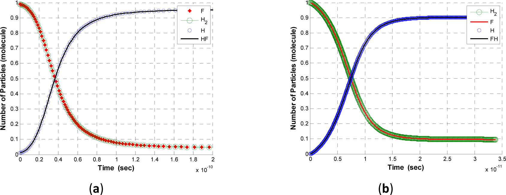

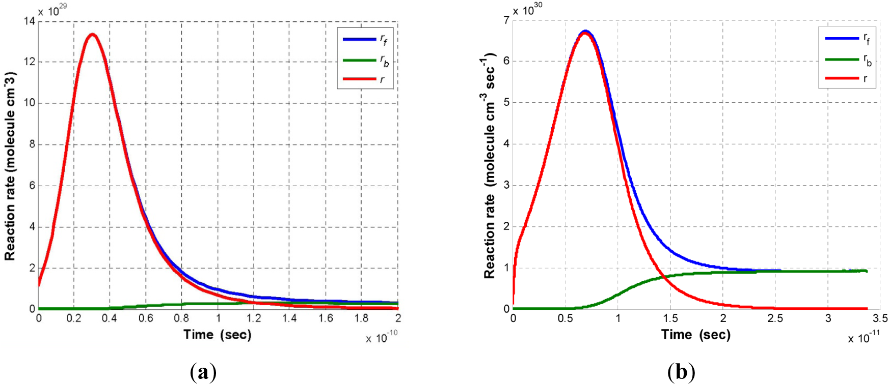


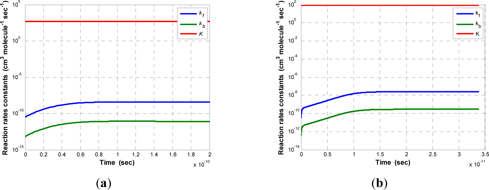
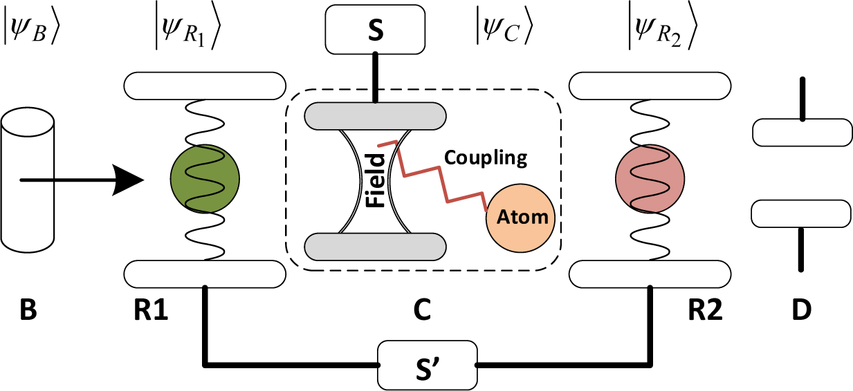
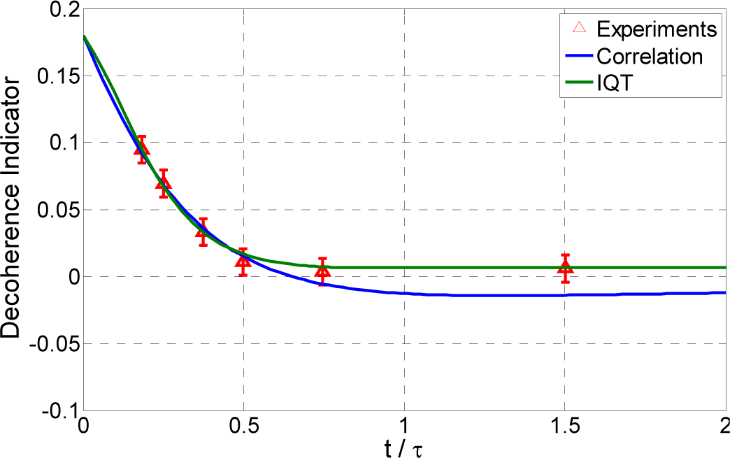
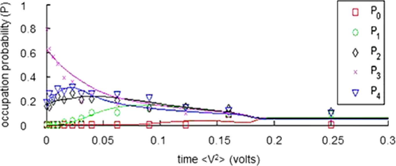
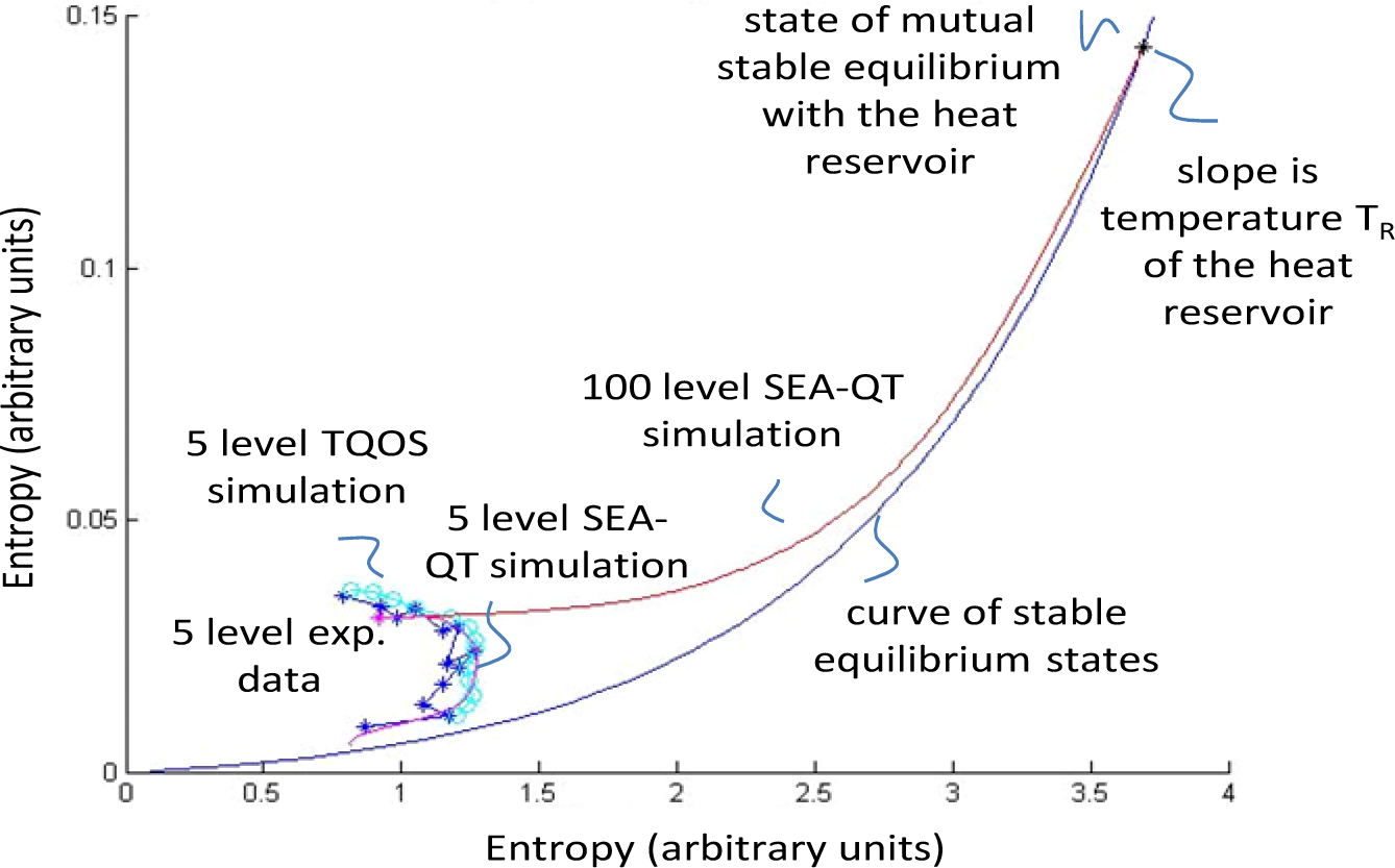
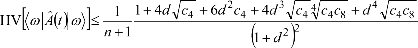
| Species | Translational Quantum #’sa | Vibrational Quantum #’s | Rotational Quantum #’s |
|---|---|---|---|
| F | 1,…,400 | ||
| H2 | 1,…,400 | 0 | 0,1 |
| FH | 1,…,400 | 0,1,2,3 | 0,1,…,7 |
| H | 1,…,400 |
aAlthough the translational principal quantum number k varies here from 1 to 400 for each species, only a sampling (30) of these quantum numbers across this range is used for each species in the finite SEA-QT model.
| kf(T)/10−11 (cm3/molecule-sec) | |||||
|---|---|---|---|---|---|
| T (K) | WHa | SBAb | HBGMc | RHPBd | WTMe |
| 298 | 2.33 | 2.48 | 2.93 | 2.81 | 2.26 |
aWurzberg and Houston [102]bStevens, Brune, and Anderson [103]cHeidner, Bott, Gardner, and Melzer [104]dRosenman, Hochman-Kowal, Persky, and Baer [105]eWang, Thompson and Miller [101].
© 2014 by the authors; licensee MDPI, Basel, Switzerland This article is an open access article distributed under the terms and conditions of the Creative Commons Attribution license (http://creativecommons.org/licenses/by/3.0/).
Share and Cite
Von Spakovsky, M.R.; Gemmer, J. Some Trends in Quantum Thermodynamics. Entropy 2014, 16, 3434-3470. https://doi.org/10.3390/e16063434
Von Spakovsky MR, Gemmer J. Some Trends in Quantum Thermodynamics. Entropy. 2014; 16(6):3434-3470. https://doi.org/10.3390/e16063434
Chicago/Turabian StyleVon Spakovsky, Michael R., and Jochen Gemmer. 2014. "Some Trends in Quantum Thermodynamics" Entropy 16, no. 6: 3434-3470. https://doi.org/10.3390/e16063434