Application of the Generalized Work Relation for an N-level Quantum System

Abstract
: An efficient periodic operation to obtain the maximum work from a nonequilibrium initial state in an N–level quantum system is shown. Each cycle consists of a stabilization process followed by an isentropic restoration process. The instantaneous time limit can be taken in the stabilization process from the nonequilibrium initial state to a stable passive state. In the restoration process that preserves the passive state a minimum period is needed to satisfy the uncertainty relation between energy and time. An efficient quantum feedback control in a symmetric two–level quantum system connected to an energy source is proposed.The maximum work formulation of the second law of thermodynamics has been generalized for transitions between nonequilibrium states [1–5]. The maximum work that can be extracted from a thermally isolated Hamiltonian system in an initial nonequilibrium state is given in terms of the relative entropy between it and a canonical distribution with an effective temperature.
It is important to recognize that the generalized second law is universal. It is a consequence of information theory (more precisely the geometry of a measure of information) and unitary time evolution. The number of degrees of freedom of a system is not important for the generalized second law. Therefore it is applicable not only to systems of interest in traditional thermodynamics but also finite systems, such as the N-level quantum system we will consider.
Our considerations are for a system with a Hamiltonian that has a time dependence associated with an external operation. The first step in extracting the maximum work from a nonequilibrium initial state is to stop its time evolution. This may be accomplished by an instantaneous stabilization process that changes the initial Hamiltonian to an effective Hamiltonian for which the nonequilibrium initial state is a stable canonical distribution. After the instantaneous stabilization an isentropic process is performed that changes the effective Hamiltonian to the final Hamiltonian.
Here a finite-time operation, including both stabilization and restoration processes, is considered for extracting work from a nonequilibrium initial state in a finite quantum system: the N–level system. We will explicitly show how the maximum work is realized in the limit of instantaneous stabilization in an exactly solvable two–level system.
It is important to confirm that the generalized work relation is consistent with known results. Several authors have rigorously shown the validity of the second law for an initial passive state in an N–level system [6–9]. (Their arguments are based on the majorization theory for N–dimensional vector space.) The maximum work from a non-passive initial state was also rigorously obtained [10,11].
It is also important to show how to extract the maximum work for a process that includes crossing of adiabatic energy levels. Work extracted from a thermally isolated equilibrium system is maximized for quasi-static realization of a given process. Allahverdyan and Nieuwenhuizen rigorously showed that this principle is violated for crossing of adiabatic energy levels[12]. We will give a process that maximizes work extraction when there is level crossing.
In recent years the optimal operation of nano- and quantum devices has become important [13–15]. From our perspective, the generalized second law can play a crucial role in the determination of optimization procedures. At the end of this letter we comment on an efficient quantum feedback control [16,17] using the instantaneous stabilizations we consider.
We consider a thermally isolated quantum Hamiltonian system. The Hamiltonian H(θ(t)) depends on time t through the parameter θ(t) following a given protocol associated with an external operation to the system. Hereafter, we abbreviate θt = θ(t) for convenience.
The time evolution of the system is governed by the quantum Liouville equation,
The density matrix at time t is given as
where the unitary time evolution operator where T means the time ordered product.
The work on the thermally isolated system from t = 0 to t = T is given as
It is important to note that the maximum work done by the system corresponds to the lowest work done on the system in our definition. Hereafter we will discuss a lower bound of the work on the system.
In the generalized second law the canonical distribution plays a crucial role even outside the context of a system in contact with a heat reservoir. The canonical distribution expresses a connection between energy (the Hamiltonian) and information (the probability distribution). Its meaning is the equilibrium state in thermodynamics but it also has meaning in a thermally isolated system. We consider the canonical distribution with the inverse of temperature α, ρcan(α, θ) = exp[α{F (α, θ)−H(θ)}] where we choose the Boltzmann constant unity and F (α, θ) ≡ −α−1 log(Tr[exp{−αH(θ)}]) is the corresponding free energy. Our definition of the temperature includes the Boltzmann constant so that the dimension of our temperature is energy. Using the canonical distribution, we can rewrite the work as
where ΔF(α) = F(α, θT) – F(α, θ0).
The von Neumann entropy of the state at time t is defined as S(t) ≡ −Tr[log(ρ(t))ρ(t)]. Using the conservation of the von Neumann entropy under unitary time evolution, S(T) = S(0), the work may be written as the important equality
where D[ρ‖ σ] ≡ Tr[{log(ρ) − log(σ)}ρ] is the non-negative quantum relative entropy[18,19]. This is an identity for any inverse of temperature α. In this equality the dissipative work W − ∆F (α) is exactly given as the difference between the initial and the final distance from equilibrium with a temperature.
Using the non-negativity of the second term in the right-hand-side of Equation (5), we obtain the generalized maximum work formulation for a nonequilibrium initial state,
where the effective temperature is uniquely determined by an isentropic condition: the von Neumann entropy for the final canonical distribution is equal to the initial von Neumann entropy , which makes the right hand side of Equation (6) maximum for .
From the isentropic condition, we can rewrite Equation (6) as
where an effective Hamiltonian is introduced to make the nonequilibrium initial state a canonical distribution: where is the corresponding free energy. The right hand side of the above inequality tells us how to realize the maximum work in two consecutive processes: (1) An instantaneous stabilization process in which we instantaneously change the initial Hamiltonian to the effective Hamiltonian at the beginning to stop the time evolution from the nonequilibrium initial state. (2) A restoration process in which the effective Hamiltonian is changed to the final one in an isentropic process.
Now we will focus on a two-level quantum system to obtain an efficient periodic operation that extracts the maximum work from a nonequilibrium initial state. We consider the following time-dependent Hamiltonian[12],
The eigenvalues of the Hamiltonian are ±∆ϵ (θ)/2. The probability amplitude for the ground state is |0, θ >= (− sin(θ), cos(θ))T and the probability amplitude for the excited state is |1, θ >= (cos(θ), sin(θ))T. The superscript T means the transposition of the vector. We choose the zero energy as the middle of the two levels to make them symmetric.
We first consider time-independent energy levels, ∆ϵ = ħω where ω is the constant angular frequency corresponding to the energy spacing. We choose the following parameter with linear time dependence for a given interval t ∈ [a, b), θt = Ω(t − a) + θa where Ω = (θb − θa)/(b − a). For this linear time-dependent Hamiltonian one can exactly derive the transition probability, which is the Rabi formula [20].
We start with the following transition amplitudes,
where η ≡ ω/(2Ω) and . The time evolution operator Uθ(θt) is the same as U(t) previously defined. Since the transition amplitudes depend on time through the parameter, we introduced Uθ(θt) to make the parameter dependence explicit. The phase factor was introduced to cancel out the parameter derivative of Uθ(θt). Therefore, the θt dependence in the right-hand-side of Equation (9) only appears in the bra-vector < k, θt|. Now we take the derivative with respect to θt to both sides of Equation (9).
where we used the completeness relation for any θ′. Using the relation ∂θ < k, θ|j, θ′ >= (2k − 1)δj,1−k for θ′ → θ, we obtain the coupled differential equations with respect to θ,
The solutions for the initial conditions, â0|0(θa) = â1|1(θa) = 1, â0|1(θa) = â1|0(θa) = 0 are given as
From Equation (11), â0|0(θ) (â1|1(θ)) is obtained from the derivatives of â1|0(θ) (â0|1(θ)) with respect to θ.
The transition probability from the excited to the ground state is given as
The survival probability is also given as PS = 1 − PT.
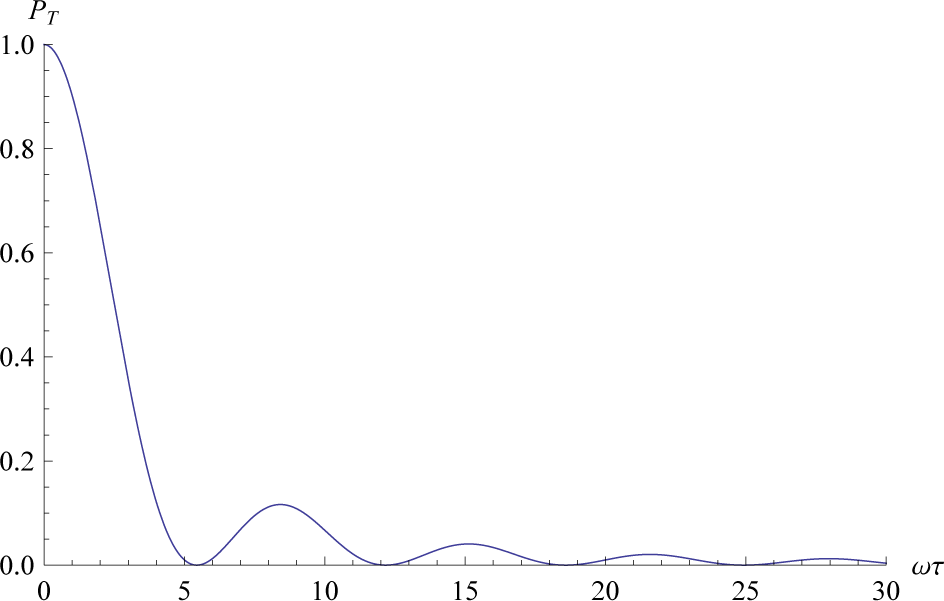
First we choose the pure excited state as a nonequilibrium initial state. This initial state is expected after energy measurement. The cyclic operation includes two processes: (1) The stabilization process for t ∈ [0, τ) in which the pure excited state becomes the ground state, the canonical distribution with zero temperature, by changing H(θ0 = 0) to H(θτ = π/2) = −H(θ0 = 0). (2) The restoration process to the original Hamiltonian without any transition to the excited state for t ∈ [τ, T). The final Hamiltonian is restored to the original Hamiltonian, H(θT) = H(θ0), for θT = π and θ0 = 0.
The transition probability for finite τ in the stabilization process is illustrated in Figure 1. When we take the limit of τ → 0, while keeping θ0 = 0 and θτ = π/2, the transition probability becomes 1 for U(θτ, τ) → 1 and the instantaneous stabilization is realized. In this limit the state does not change, ρ(τ) = ρ(0), but the energy switches sign, H(θτ) = −H(θ0).
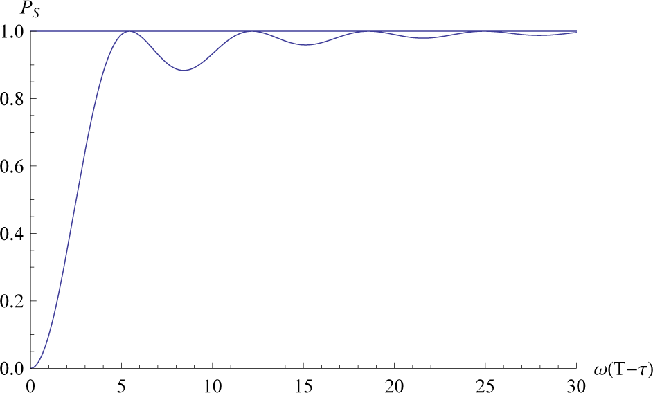
The survival probability in the restoration process is illustrated in Figure 2 where T − τ is the period of the restoration process. In the limit of the quasi-static process, T − τ → ∞, there is no transition to the excited state and the ground state is preserved. As is seen in Figure 2, there are shorter periods for a restoration that preserves the ground state (PS = 1). The shortest time for the restoration is realized by , where in Equation (12) for θ − θa = π/2 and η = ω(T − τ)/π.
The previous argument can be generalized to an arbitrary nonequilibrium initial state. Without loss of generality, a nonequilibrium initial state can be written as the superposition of orthogonal pure states,
where we define the zero-th and first pure states based on the occupation probability of the first pure state being equal or less than the zero-th, p0 ≥ p1 ≥ 0 (p0 + p1 = 1). Since the states we consider are density matrices, they are operators in the Hilbert space of probability amplitudes; in particular, the pure state is a projection operator.
In the stabilization process, the dominant zero-th state is changed to the ground state. From the property of the unitary time evolution, the first state becomes the excited state after this stabilization process. Then, the state ρ(τ) becomes the canonical distribution with the effective temperature . To realize the instantaneous stabilization, we take the limit of τ → 0 while keeping θ0 = 0 and θτ = ϕ. In this limit, ρ(τ) = ρ(0) and the Hamiltonian becomes the effective Hamiltonian given as
The transition probability from the zero-th pure state to the ground state for finite τ, PT = |−â0|1 sin(ϕ)+ â0|0 cos(ϕ)|2, is illustrated in Figure 3.
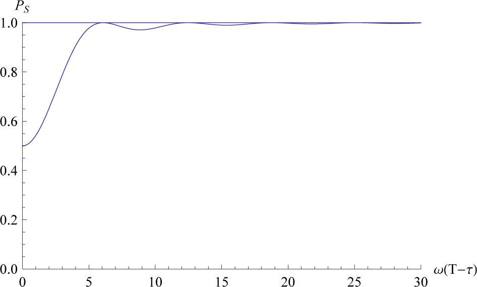
In the restoration process, the final Hamiltonian is restored to the original Hamiltonian, H(θT) = H(θ0), for θT = π. As is seen in Figure 4, the shortest time to avoid any transition is realized by where PS = |â0|0|2 = 1.
The maximum work is given as W = − ħω sin2(ϕ). This is consistent with results in [10,11]. At first glance we can extract the maximum energy more efficiently for wider level spacing, ħω. However, it is important how long it takes to re-excite the state to extract the work repeatedly. The relaxation time is crucial for the re-excitation using a heat reservoir as will be discussed later.
Now we consider an efficient periodic operation including a process with level crossing to obtain the maximum work. We choose ∆ϵ = −2 ħωθ/π in the Hamiltonian. The eigenvalues of the Hamiltonian are ± ħωθ/π so the level crossing occurs at θ = 0. We choose the time-dependent parameter for t ∈ [a, b) as θt = Ω(t−a)+θa. As was shown by Allahverdyan and Nieuwenhuizen[12], the transition probability can be rigorously obtained even in a process with level crossing. Therefore we can explicitly show both the stabilization process and the restoration process.
We consider the following transition probability similar to the previous case,
We obtain the coupled differential equations,
The solutions can be written as
where c1 and c2 are constants, He is a Hermite polynomial, and F1 is a confluent hypergeometric function of the first kind [21]. They are generalized for complex parameters and complex variable.
The transition probability from the initial excited state to the final ground state is given as PT = |â1|1(θb)|2 and the survival probability PS = |â0|1(θb)|2 = 1 − PT. Notice that the initial state is same as the final state in the transition probability. This comes from the fact that the initial excited state becomes the final ground state because of the level crossing.
We first consider the stabilization process for t ∈ [0, τ). The instantaneous stabilization can be realized even in a process with level crossing. For the nonequilibrium initial state defined in Equation (14), we choose θ0 = −π/2 and θτ = φ > 0 and take the limit of τ → 0. Then, ρ(0) = ρ(τ) and
The transition probability for finite τ, PT = | − â1|1 sin(ϕ) + â1|0 cos(ϕ)|2, is shown in Figure 5.
We consider the restoration process to the original Hamiltonian for t ∈ [τ, T). The restoration of the original Hamiltonian, H(θT) = H(θ0), is realized for θτ = ϕ and θT = −π/2. We can make an efficient process without any transition between the two levels by choosing the interval T − τ for which PS = |â0|1|2 = 1 as shown in Figure 6.
As was pointed out by Allahverdyan and Nieuwenhuizen [12], if level crossing occurs work extraction is not always maximized by a quasi-static operation. Using a non-quasi-static operation such as the instantaneous stabilization we can extract the maximum work in a process with level crossing. The level crossing occurs within the stabilization process. Any effect of the level crossing turns out to be negligible in the instantaneous limit. The instantaneous stabilization was originally introduced to prevent spontaneous relaxation of a nonequilibrium thermodynamic system. It also prevents any loss of work in a process with level crossing for an N–level quantum system.
In order to extend our argument for N = 2 to a general N we first have to modify the generalized maximum work formulation for a general N–level system. For N = 2, we can take any nonequilibrium initial state to the final canonical distribution by adjusting the effective temperature. However, we cannot do this for a greater N. The set of eigenvalues of the initial density matrix is preserved under a unitary time evolution. If we can take a nonequilibrium initial state to the final canonical distribution, the set of eigenvalues of the initial density matrix must be same as the set of the final canonical distribution in the diagonal representation. Since the final Hamiltonian (the set of final energy levels) is given, we cannot take an arbitrary nonequilibrium initial state to the final canonical distribution using any unitary time evolution.
Fortunately, we can take any nonequilibrium initial state to the final passive state and the second law for a passive initial state was established in an N–level quantum system [6–9]. A passive state satisfies the following properties: (1) It is simultaneously diagonalizable with the Hamiltonian so it can be written in terms of a sum of energy eigenstates. (2) It is determined by a series of occupation probabilities for each energy level. (Here we assume no degeneracy with respect to energy levels.) (3) The series of occupation probabilities is monotonically decreasing in the wide sense with respect to the level of energy. (The occupation probabilities of the nth energy level is equal or greater than the n + 1th energy level for n = 0, 1, 2, …, N − 1.)
Similar to an initial canonical distribution, we can not obtain work from an initial passive state using any periodic operation,
where ρpassive(t) is a passive state at time t.
Using the above inequality we obtain the generalized maximum work formulation for a nonequilibrium initial state in an N–level system as
where is the effective Hamiltonian for which the nonequilibrium initial state is written as a passive state in terms of the effective Hamiltonian. The maximum work can be extracted in two consecutive processes: the instantaneous stabilization and an isentropic process such as a quantum quasi-static process from the effective passive state to the final passive state.
Finally, we consider a periodic operation to obtain the maximum work from a nonequilibrium initial state in an N–level system. The periodic operation is divided into two processes: the instantaneous stabilization and the restoration process to the original Hamiltonian.
Suppose both the initial Hamiltonian and the nonequilibrium initial distribution are written as a sum of pure eigenstates in each diagonal representation,
where ϵn < ϵn+1 (n = 0, 1, …, N −1) and pure eigenstates, |ψj > < ψj| (j = 0, 1, …, N −1), are ordered from the largest occupation probability p0 to the smallest occupation probability pN−1. Then, we choose the effective Hamiltonian as
The instantaneous stabilization is realized by instantaneously changing from the initial Hamiltonian to the effective Hamiltonian. The nonequilibrium initial state is kept in the sudden approximation as was explicitly shown for the two–level quantum system.
In the restoration process, we change the effective Hamiltonian to the original Hamiltonian. The state remains passive without any transition during the minimum period ħ/∆ϵ expected from the uncertainty relation.
To close we comment on an efficient quantum feedback control using the instantaneous stabilizations. The system needs to be coupled to an energy source, such as a heat reservoir, to extract the maximum work repeatedly. We can obtain the maximum work from an initial excited state using the instantaneous stabilization. If the system is symmetric, such as a two–level quantum system, the Hamiltonian after the instantaneous stabilization is the same form as the original Hamiltonian. Then, we may skip the restoration process. After re-excitation by the energy source, we repeat the instantaneous stabilization. Since a real stabilization is an almost instantaneous process, we can control the system even though it is coupled to an energy source. The minimum period is determined by the re-excitation time, such as the relaxation time Since our argument is not restricted within thermodynamics, we can choose any energy source such as light from sun to make the re-excitation time much shorter. We expect our efficient quantum process plays an important role in a quantum dot solar cell.
We have to measure the quantum system to know if the system is in the excited state. The whole process including quantum measurements is called quantum feed back control[16,17,22]. Toyabe et al. reported their experimental results[23]. We interpret their experiment as a demonstration of our efficient quantum feedback control using instantaneous stabilizations.
Acknowledgments
Hiroshi Hasegawa and Kazuma Takara thank Hal Tasaki for his important suggestions. This work was performed under the Cooperative Research Program of “Network Joint Research Center for Materials and Devices”.
Conflicts of Interest
The authors declare no conflict of interest.
References
- Hasegawa, H.-H.; Ishikawa, J.; Takara, K.; Driebe, D. Generalization of the second law for a nonequilibrium initial state. Phys. Lett. A 2010, 374, 88–92. [Google Scholar]
- Takara, K.; Hasegawa, H.-H.; Driebe, D. Generalization of the second law for a transition between nonequilibrium states. Phys. Lett. A 2010, 375, 1001–1004. [Google Scholar]
- Esposito, M.; Lindenberg, K.; van den Broeck, C. Entropy production as correlation between system and reservoir. New J. Phys 2010, 12, 013013. [Google Scholar]
- Esposito, M.; van den Broeck, C. Second law and Landauer principle far from equilibrium. Europhys. Lett 2011, 95, 40004. [Google Scholar]
- Deffner, S.; Jarzynski, C. Information Processing and the Second Law of Thermodynamics: An Inclusive, Hamiltonian Approach. Phys. Rev. X 2013, 3, 041003, and references therein. [Google Scholar]
- Lenard, A. Thermodynamical proof of the Gibbs formula for elementary quantum systems. J. Stat. Phys 1978, 19, 575–586. [Google Scholar]
- Pusz, W.; Woronowicz, S. Passive states and KMS states for general quantum systems. Commun. Math. Phys 1978, 58, 273–290. [Google Scholar]
- Allahverdyan, A.; Nieuwenhuizen, Th. A mathematical theorem as the basis for the second law: Thomson’s formulation applied to equilibrium. Physica 2002, A305, 542–552. [Google Scholar]
- Tasaki, H. Statistical mechanical derivation of the second law of thermodynamics. arXiv 2000, arXiv. cond-mat/0009206v2.
- Hatsopoulos, G.; Gyftopoulos, E. A unified quantum theory of mechanics and thermodynamics. Part IIa. Available energy. Found. Phys 1976, 6, 27–141. [Google Scholar]
- Allahverdyan, A.; Balian, R.; Nieuwenhuizen, Th. Maximal work extraction from finite quantum systems. Europhys. Lett 2004, 67, 565. [Google Scholar]
- Allahverdyan, A.; Nieuwenhuizen, Th. Minimal work principle: proof and counterexamples. Phys. Rev 2005, E71, 046107. [Google Scholar]
- Jarzynski, C. Equalities and Inequalities: Irreversibility and the Second Law of Thermodynamics at the Nanoscale. Annu. Rev. Condens. Matter Phys 2011, 2, 329–351. [Google Scholar]
- Campisi, M.; Hänggi, P.; Talkner, P. Colloquium: Quantum fluctuation relations: Foundations and applications. Rev. Mod. Phys 2011, 83, 771. [Google Scholar]
- Deffner, S.; Jarzynski, C.; del Campo, A. Classical and Quantum Shortcuts to Adiabaticity for Scale-Invariant Driving. Phys. Rev. X 2014, 4, 021013. [Google Scholar]
- Sagawa, T.; Ueda, M. Second Law of Thermodynamics with Discrete Quantum Feedback Control. Phys. Rev. Lett 2008, 100, 080403. [Google Scholar]
- Sagawa, T.; Ueda, M. Minimal Energy Cost for Thermodynamic Information Processing: Measurement and Information Erasure. Phys. Rev. Lett 2009, 102, 250602. [Google Scholar]
- Breuer, H.; Petruccione, F. The Theory of Open Quantum Systems; Oxford University Press: Oxford, UK, 2006. [Google Scholar]
- Deffner, S.; Lutz, E. Generalized Clausius inequality for nonequilibrium quantum processes. Phys. Rev. Lett 2010, 105, 170402, and references therein. [Google Scholar]
- Loudon, R. The Quantum Theory of Light; Oxford University Press: Oxford, UK, 2000. [Google Scholar]
- Abramowitz, M.; Stegun, I.A. Handbook of Mathematical Functions with Formulas, Graphs, and Mathematical Tables, 10th ed.; United States Government Printing: New York, NY, USA, 1984. [Google Scholar]
- Jacobs, K. Second law of thermodynamics and quantum feedback control: Maxwell’s demon with weak measurements. Phys. Rev. A 2009, 80, 012322. [Google Scholar]
- Toyabe, S.; Sagawa, T.; Ueda, M.; Muneyuki, E.; Sano, M. Experimental demonstration of information-to-energy conversion and validation of the generalized Jarzynski equality. Nat. Phys 2010, 6, 988–992. [Google Scholar]


© 2014 by the authors; licensee MDPI, Basel, Switzerland This article is an open access article distributed under the terms and conditions of the Creative Commons Attribution license (http://creativecommons.org/licenses/by/3.0/).
Share and Cite
Ishikawa, J.; Takara, K.; Hasegawa, H.-H.; Driebe, D.J. Application of the Generalized Work Relation for an N-level Quantum System. Entropy 2014, 16, 3471-3481. https://doi.org/10.3390/e16063471
Ishikawa J, Takara K, Hasegawa H-H, Driebe DJ. Application of the Generalized Work Relation for an N-level Quantum System. Entropy. 2014; 16(6):3471-3481. https://doi.org/10.3390/e16063471
Chicago/Turabian StyleIshikawa, Junichi, Kazuma Takara, Hiroshi-H. Hasegawa, and Dean J. Driebe. 2014. "Application of the Generalized Work Relation for an N-level Quantum System" Entropy 16, no. 6: 3471-3481. https://doi.org/10.3390/e16063471
APA StyleIshikawa, J., Takara, K., Hasegawa, H.-H., & Driebe, D. J. (2014). Application of the Generalized Work Relation for an N-level Quantum System. Entropy, 16(6), 3471-3481. https://doi.org/10.3390/e16063471