Entropy in the Critical Zone: A Comprehensive Review


Abstract
: Thermodynamic entropy was initially proposed by Clausius in 1865. Since then it has been implemented in the analysis of different systems, and is seen as a promising concept to understand the evolution of open systems in non-equilibrium conditions. Information entropy was proposed by Shannon in 1948, and has become an important concept to measure information in different systems. Both thermodynamic entropy and information entropy have been extensively applied in different fields related to the Critical Zone, such as hydrology, ecology, pedology, and geomorphology. In this study, we review the most important applications of these concepts in those fields, including how they are calculated, and how they have been utilized to analyze different processes. We then synthesize the link between thermodynamic and information entropies in the light of energy dissipation and organizational patterns, and discuss how this link may be used to enhance the understanding of the Critical Zone.1. Introduction
The Earth’s Critical Zone (CZ) is defined as the heterogeneous, near surface environment in which complex interactions involving rock, soil, water, air, and living organisms regulate the natural habitat and determine the availability of life-sustaining resources [1]. The CZ is the result of complex interactions of physical, chemical, and biological processes that have taken place over an evolutionary time scale [2]. These interactions have been driven by energy, mass, entropy, and information fluxes, and the result is heterogeneous but organized structures that regulate the flow of energy down the gradients of various kinds [2,3].
Based on the role that mass, energy, entropy, and information have on the evolution of the CZ, thermodynamics and information principles have always been considered as potential tools that would allow us to better understand the evolution and organization of the CZ [4,5]. In particular, the second law of thermodynamics and the ubiquitous production of thermodynamic entropy in the universe has been conceived as fundamental principle that is connected with the evolution of the CZ [2]. In addition, the organized patterns and information contained in the CZ have been analyzed with Shannon (information) entropy or derived concepts. Therefore, an extensive number of studies have been published where thermodynamic entropy or information entropy have been used to analyze various processes in the CZ.
In this paper, we review these previous studies where thermodynamic entropy, information entropy, or their derived concepts have been attempted to understand the CZ. In particular, we analyze possible connections between these two concepts. We first summarize previous applications of thermodynamic and information entropies as they were applied to the CZ. Afterwards, we discuss how these concepts may be related and how we may use this connection to advance the understanding of the CZ.
2. Thermodynamic Entropy Applied to the Critical Zone
In this section we review previous studies where thermodynamic entropy or related concepts such as exergy have been used in different applications in the CZ. It is worth mentioning that the CZ is a complex system with many interactions at different time and spatial scales. Therefore, physical laws applied to the CZ are generally stated in a idealized conditions, which must be applied with caution. We start from the conservation equations of mass and energy, and then we use the entropy balance equation to define a general expression for the production of entropy in the CZ. Afterwards, we summarize different approaches where the production of entropy in the CZ has been computed. The Online Supplement Section 1 presents a brief introduction to the concept of thermodynamic entropy in open systems.
The mass, energy, and entropy balance equations defined in the Online Supplement Section 1 for open systems can be applied for a particular spatial domain Vcz that defines the control volume of the CZ. Therefore, in order to analyze the entropy budget in the CZ it is important to define the boundaries that delineate the CZ. The selection of these boundaries could be arbitrary but important since they define the control volume and the location where various fluxes take place. The lower boundaries were defined by Kleidon et al. [6] as the bottom of the regolith, and the upper boundary as an imaginary limit right above the canopy. A similar control volume was conceptualized by Rasmussen et al. [3] and Lin [7]. Watersheds could be an interesting spatial unit to delineate the CZ, as they are a fundamental spatial unit not only in hydrology but in many other fields related to CZ processes. Reggiani et al. [8–10] proposed this conceptualization by incorporating the concept of representative elementary watershed REW as a main spatial unit in the budget of entropy. However, the lateral boundaries that delineate the CZ could vary according to the purpose of each particular study, and may range between a geographic cell, a watershed, or an entire continent (Figure 1).
In this study we use the notation of I, J, and L to represent the fluxes of mass, energy, and entropy, respectively. A comprehensive list of the symbols used in this study is displayed in the Online Supplement Section 6.
2.1. Mass, Energy, and Entropy Balance
The mass balance for a particular control volume Vcz that delineates the CZ can be calculated with Equation (1), where the total mass change in the CZ will be equal to the summation of all mass changes in all the components:
In this equation MT,cz is the total mass in Vcz, mcz refers to the mass content in a elemental volume where equilibrium conditions are assumed to be valid. Index k refers to a particular component of the CZ, Mk is the molar mass of component k, and nk is the number of moles of component k in the elemental volume. The change of mass of a particular component k in the elemental volume is equal to the net flux across the boundary and a source or sink term related to all chemical reactions Nk,cz within Vcz where component k is involved. Acz represents the total surface area of the CZ. Terms dA and refer to an elemental area that is part of Acz, and a unit normal vector field to Acz respectively. Terms υj and νj,k are the velocity of the chemical reaction j, and the stoichiometric coefficients of component k in the reaction j, respectively. A similar approach can be used to quantify the energy balance:
Here ET,cz is the total energy in the control volume, and ez refers to the energy content at the local domain. The net flux J represents the net flux of energy across the surface of the CZ, including heat, radiation, and kinetic and internal energy of mass fluxes. The balance of entropy for a en elemental volume in the CZ is given by (See Online Supplement Section 1):
where scz is the entropy content at a local domain, and L represents the net flux of entropy. The term σcz refers to the production of entropy at a local domain. We can write Equation (3) as:
In this equation Jq is the flux of heat, Ik refers to the flux of mass of component k, sk is the molar entropy in component k, and Lrad is the flux of entropy due to radiation fluxes. The ratio Ik/Mk is the molar flux of component k.
Equation (4) is the general form of the entropy balance at a local domain in the CZ. It is worth mentioning that this Equation represents all the possible fluxes but not every local domain in the CZ will experience all these fluxes. Note that in Equation (4) the local entropy production is splitted in two components, σcz,rad and σcz,int. Term σcz,rad refers to the local entropy production associated with an instantaneous transformation of radiation in the surface, and σcz,int refers to the local production of entropy related to internal processes. Radiation is an important part of the energy balance in the CZ. On the one hand, a significant fraction of the incoming radiation that is continuously reaching the CZ is dissipated instantaneously in other forms of energy such as latent heat (LE), sensible heat (HH), and emitted longwave (LW) radiation. There is a significant entropy production associated with this dissipation because it involves a transformation of shortwave (SW) radiation with low entropy to other forms of energy with higher entropy (such as heat and LW radiation). In this paper we call this entropy production σcz,rad. Although σcz,rad could be affected by the structure and functioning of the CZ, this entropy is not directly produced by internal processes that occur within the CZ; rather it is an instantaneous transformation of radiation at the surface of the CZ. On the other hand, there is a flux of energy (chemical, heat, and kinetic) that is continuously absorbed by the CZ. This energy drives various processes that occur within the CZ and produce entropy. In this paper we call this entropy production σcz,int. Equation (5) describes the formulation for σcz,int under the presence of the Earth’s gravitational field:

There are five main components associated with σcz,int. Table 1 and Figure 2 explain these components in more detail. The derivation of Equation (5) is based on Kondepudi and Prigogine [11] and is presented in the Online Supplement Section 2. Note that σcz,int is always positive following the second law of thermodynamics. We can observe the complexity associated with the CZ. Besides, the high production of entropy linked to the transformation of SW radiation fluxes at the surface (σcz,rad), the production of entropy within the CZ (σcz,int) is associated with many different processes (Equation (5), Table 1, Figure 2).
Equations (4) and (5) are the fundamental equations for the entropy balance in the CZ. However, note that both σcz,rad and σcz,int refer to entropy productions defined over a local domain. It is possible to define a generation of entropy for the entire CZ delineated by Vcz, and over a time scale τ associated with a particular process as [12–14]:

Similarly, this generation of entropy can be divided in one part that is linked to internal processes within the CZ, and other part that is linked to the instantaneous transformation of SW radiation at the surface:
2.2. Exergy Balance
Exergy is defined as the maximum work that can be extracted by an overall system composed of a system and its environment as both comes into equilibrium [15]. Exergy provides a magnitude of the available energy that can be used as a work, and therefore it is considered as an extended definition of free energy for open systems. Considering the CZ as an open control volume that exchanges fluxes of heat, mass, and radiation with a reference idealistic environment it is possible to define the balance of exergy in the CZ from Equations (2), (4) and (6) as:

where Eex is the exergy content in the CZ, and hk is the molar enthalpy of constituent k. Term To refers to the temperature of a hypothetical reference environment. Terms RF and Tsource represent the radiation factor and temperature of the body that is emitting the radiation (See Online Supplement Section 3). RF and Tsource vary according to the type of radiation, and usually in CZ studies they are differentiated for SW and LW radiation.
A main hindrance in the analysis of exergy in the CZ is the environment [16]. As shown in Equation (8) in order to compute the exergy balance in the CZ, some properties of the environment are needed. There are different alternatives that could considered as the environment of the CZ such as the atmosphere, a nearby CZ, or even the Sun. Therefore, it is challenging to define specific properties such as the temperature for the environment of the CZ in order to perform a complete exergy analysis using Equation (8). Although it is difficult to analyze the balance of exergy in the CZ, it is possible to link the entropy generation with the destruction of exergy [13]. According to the Gouy - Stodola theorem the destruction of exergy due to irreversible processes is proportional to the generation of entropy and is given by [12,14]:
where Γcz is the destruction of exergy due to irreversible processes in the CZ. Similar approaches have been implemented in the CZ [3,17].
Note that when the entire CZ is analyzed as a system the net work performed by the CZ over a reference environment is negligible and is not included in the energy and exergy balances in Equations (2) and (8) respectively. In other words, all the exergy that is reaching the CZ is destroyed in two main forms: (i) at the surface due to an instantaneous transformation of SW radiation (Γcz,rad); and (ii) by internal processes within the CZ (Γcz,int), some of which use the exergy that is being captured to produce work but this work is in turn dissipated as heat and leaves the CZ in the form of heat. Based on Equations (7) and (9) it is also possible to have an expression for these two forms of exergy destruction as:
2.3. Computation of Thermodynamic Entropy in the Critical Zone
Quantification of thermodynamic entropy in the entire CZ is challenging as it involves a complex and heterogeneous control volume. This quantification can be performed with Equations (4) and (5) by selecting a proper control volume and computing the fluxes of entropy across the boundary of this control volume (Figure 3a). In order to use this approach the rate of change of the total entropy in the control volume of the CZ (dST,cz/dt) is needed or a steady state assumption (dST,cz/dt = 0; Online Supplement, Section 1.4) can be assumed (e.g., Wu and Liu [18]). Note that the CZ is continuously evolving and will never be in a true steady state condition. However, the steady state assumption is a mathematical simplification that allows us to have a solution by considering a close-to-equilibrium steady state condition in the CZ where annual changes are not significant. The production of entropy for any particular control volume in the CZ is associated with infinity number of processes. Sometimes we are interested in the analysis of the most prominent processes in the entropy budget (Figure 3b). In this case, the entropy production related to specific processes are calculated (e.g., Kleidon et al. [19]). In this section we review some of the previous approaches that have computed thermodynamic entropy or exergy in different parts of the CZ. In Table 2 we provide a description of important concepts that have been utilized in the CZ.
2.3.1. Vertical Domain
The consideration of a vertical domain where horizontal fluxes are neglected allows to simplify the balances of mass and energy in the CZ. According to Volobuyev [20] the mass balance in the CZ over a vertical domain including the most prominent fluxes can be expressed as:
where terms I’s refer to net mass fluxes associated with various components. The subscripts H2O, ELV, and GEO refer to water, and physical and chemical denudation respectively. The last term is a summation that accounts for the fluxes of all the other components not directly considered.
Similarly, the energy balance can be computed by considering the most prominent fluxes:
where JQ,LE and JQ,H are the LE and HH heat fluxes released from the surface of the CZ respectively. Terms JSW and JLW are the fluxes of energy in the form of SW and LW radiation, respectively. Term is a net flux of energy associated with incoming and outgoing fluxes of water. Differences in energy content between incoming and outgoing fluxes of water occurs due to dissipation of potential and kinetic energy of water within the CZ. Note that does not include the energy associated with LE which is considered separately in JQ,LE. Terms ck and uk accounts for the average kinetic and internal energy respectively of all the other mass components k that flow into the CZ. Terms JELV and JGEO are the heat fluxes associated with physical and chemical denudation. A description on how JELV and JGEO can be estimated is given in Rasmussen et al. [3]. Note, that the net radiation Rn can be expressed as:
Rn is a remaining fraction of the incoming radiation that is dissipated in other forms of energy such as heat and photosynthesis in the CZ. Note that:
where JQ,resp is the flux of heat released after respiration and work of biological systems is performed. Term represents an additional flux of heat within the CZ released by dissipation of kinetic and potential energy of water. Term JSW,pho is the flux of SW radiation taken through photosynthesis. Terms JQ,G and JQ,atm are the ground heat flux and the flux of heat to the atmospheric part of the CZ respectively. Using Equations (12)–(1) the energy balance can also be expressed as:

Note that the flux of heat released after respiration (JQ,resp) is from living systems within the CZ to the soil and the atmospheric part of the CZ. Also, the flux of heat is from water stored within the CZ to the soil and atmospheric part of the CZ. Therefore, these heat fluxes are still within the control volume of the CZ and are already included in JQ,G and and JQ,atm. This explains why they are deducted in Equation (1) from the energy balance inside the CZ. Term accounts for the net energy flux into the CZ due to water fluxes. Term JBIO is the net energy flux of the living systems in the CZ. Equations (12) and (1) are equivalent. However, Equation (1) accounts for only those fluxes that are absorbed by the CZ, and do not consider the fraction of the incoming radiation fluxes that are dissipated instantaneously. Using the same approximation of a vertical domain and neglecting horizontal fluxes, the entropy balance and generation of entropy in the CZ can be computed from the energy balance in Equation (12) as:

In this equation refers to the total entropy generated by the CZ, and L′ sterms refer to all the respective fluxes of entropy. Similarly, it is also possible to perform an entropy balance using the energy balance in Equation (1).

Term (LBIO) in Equation (1) is the net entropy flux associated with living systems in the CZ. Also, note that the entropy generated in Equations (1) and (1) are different. Equations (12) and (1) are equivalent because energy is a conservative quantity. However Equations (1) and (1) are not the same because there is an entropy production associated with the dissipation of SW radiation, and this entropy is not included in Equation (1). The total entropy generated is, therefore, divided in two (Equation (4)).
Previous studies such as Rasmussen et al. [3] have used Equation (1) to examine the energy flowing trough the CZ neglecting radiation fluxes. Other studies such as Holdaway et al. [21] have implemented Equation (12) including radiation fluxes. The establishment of micrometeorological towers and the implementation of the eddy covariance methods in past years have improved our quantification of the energy fluxes at the surface [22] allowing a more detail quantification of the entropy budget. The energy balance in Equations (12) and (1) can be computed from data recorded in micrometeorological towers if JGEO and JELV are neglected. This approach was implemented by Holdaway et al. [21] to solve Equation (1) and compute based on information recorded in different towers in the Amazon that had been established under ecosystems at different stages of development. They observed a higher under the most developed ecosystems (e.g., trees over grasses).
2.3.2. Entropy of Radiation
When the control volume under consideration spans the entire CZ, or includes the surface (Figure 3) the radiation component plays an important part of the entropy budget. Therefore, in order to compute in Equation (1) we must quantify the fluxes of entropy that are associated with radiation. The contributions from previous studies [18,23,24] (see Online Supplement, Section 3) that were able to obtain a simplified formulation to quantify the entropy fluxes in radiation are particularly important. Some approaches have calculated the entropy of radiation using a Clausius approximation (dS = dQ/T). However, this approach neglects what we call in this study the radiation factor, , which is approximately (4/3). This extra (1/3) may represent an important fraction in the entropy budget and .
Initial approaches that quantify the entropy budget by incorporating radiation fluxes were developed by Aoki [25,26] at the plant leaf scale (Figure 3). These approaches included the most important fluxes of energy reaching and leaving the leaf surface such as direct and diffuse SW radiation, LW radiation, and heat fluxes. A precise estimation of entropy in the incoming SW radiation is particularly important because it is the source of energy with the lowest entropy. According to Aoki [27] the flux of entropy in SW radiation is given by:
In this equation LSW and JSW are the fluxes of entropy and energy respectively associated with SW radiation. Terms esolar and ssolar are the solar constants of first and second kind respectively. Aoki quantified the entropy in diffuse SW, and LW radiation using the approach developed by Landsberg and Tonge [23]. He was able to show that the thermodynamic entropy difference between the incoming and outgoing fluxes was negative, resulting in a net increase of entropy which was expected based on the second law of thermodynamics. These studies pointed the role of solar energy in the production of entropy from the leaf. Solar energy controls the entropy budget as it has much lower entropy than LW radiation or heat. They found that the entropy production from the leaf surface increased linearly with solar energy . Similar results were found in different earth surface systems [28,29].
2.3.3. Atmosphere—Soil Interaction
The CZ and the atmosphere are coupled. As a result of this coupling there is a continuous exchange of heat, mass, and momentum fluxes that maintain both systems far from equilibrium. According to Pauluis and Held [30] the atmospheric circulation operates as a dehumidifier that induces dry air. Dry air in the atmosphere is originated by precipitation which is an outgoing flux of moisture that occurs as a result of radiative cooling. Both the lifting of air masses with vapor and the occurrence of precipitation induces a reduction of water vapor in the lower atmosphere that enhances the gradient in water potential between the CZ and the atmosphere. This gradient is used by the plants to transpire water from the soil. In turn, transpiration fluxes intensify the water potential gradients in the soil enhancing the infiltration of moisture which is one of the most significant sources of work driving the evolution of soils in the CZ [31].
In addition, the mixing of saturated air from the transpiration of plants (or soil evaporation) and unsaturated air in the boundary layer above the canopy results in a significant production of entropy. This production of entropy is an important component of the global water cycle entropy budget and can be computed as [19]:
where RHa is the relative humidity of atmospheric air at the air temperature, RHs is the relative humidity of close to saturation air, Rυ is the gas constant for water vapor, and is the flux of water related to transpiration (or evaporation).
Thermodynamic entropy in the atmosphere has been studied extensively (See Ozawa et al. [32]). In the atmosphere the dissipation of kinetic energy represents a prominent source of entropy generation. Therefore, the generation of entropy for a control volume Vatm in the atmosphere could be approximated as [33]:
In this formulation mass, and radiation fluxes are neglected (See Equation (5)). Similar approaches could be considered to analyze the atmospheric part of the CZ. However, the atmospheric part of the CZ is strongly influenced by the surface and fluxes of mass could become an important source of entropy production.
2.3.4. Soils
Soils are an important component of the CZ that sustains the highest level of biodiversity in the Earth and accounts for thousands of interactions between different species of microorganisms, soil fauna, and plant roots [7]. The structure of soils follow distinct patterns of organization that resulted from a self-organizing process over thousands of years. This self-organization is driven by fluxes of exergy and entropy, and therefore thermodynamics has been considered an important element in pedogenesis. Some review studies [7,34,35] have discussed the role of themodynamics in the understanding of the mechanisms associated with soil formation. Therefore, in this section we focus in the description of the most influential studies related to thermodynamic entropy and soil formation.
Some initial studies have explored the impact of energy in the formation of soils [20,36]. In particular, the approach introduced by Volobuyev [20] presented a novel formulation by performing an energy balance in the soil where the total available energy is allocated in different processes such as weathering, leaching, evapotranspiration, and chemical transformations related to organic matter. In this study he claimed that evapotranspiration is by far the most prominent component of this energy budget. On the contrary, the energy associated with biological processes accounts for a small fraction. However, the information used by Volobuyev to analyze energy patterns was limited. In recent years the availability of micrometeorological towers, together with more precise numerical models [3,22,37,38] have allowed us to have a more detailed understanding of the energy balance in the surface. Although the energy associated with evapotranspiration fluxes is significant, it is mostly linked to the dissipation of incoming fluxes of radiation at the surface (Equation (1)). On the other hand, other processes such as biochemical fluxes from photosynthesis associated with biological processes, percolation of water, and fluxes of heat into the CZ are major components of the internal production of entropy within the CZ (Equation (1)) and regulate the evolution and organizational patterns observed within the CZ.
Previous studies have quantified the standard free energy, enthalpy, and thermodynamic entropy for different minerals [39]. However, it is challenging to scale and conceptualize the entropy for the entire soil. An initial approach by Volobuyev et al. [40] scaled up the chemical potentials by performing a direct summation of the chemical potentials in the different minerals constituting a given soil:
The term Fs refers to the free energy in the entire soil domain. The same approach was implemented in different types of soils and Volobuyev et al. [40] were able to find important patterns. On the one hand, soils with significant quantities of residual products resulting from weathering of the parent material such as SiO2, AlO3, Fe2O3, and CaCO3 have the lowest values of Gibbs free energy. On the other hand, less weathered soils such as vertisols results in higher values of Gibbs free energy. These results show that higher entropy is reflected in minerals more resistant to weathering [35]. Another approach dealing with thermodynamic entropy in soils was performed by Smeck et al. [41]. In this formulation they hypothesized that the change of entropy content in the soil (∆Ss) is associated with the orderliness that is observed in the soil. According to Smeck et al. [41] the relative entropy change (∆Ss) in the soil will be positive when it results in a less ordered structure, and it will be negative when it results in a more ordered structure. Therefore, processes such as weathering and physical mixing enhances ∆Ss, while other processes such as eluviation-illuviation, weathering of secondary minerals, and accumulation of organic matter reduces ∆Ss.
However, Minasny et al. [35] pointed that the patterns expected from the formulations proposed by Volobuyev et al. [40] and Smeck et al. [41] are different. For instance, highly weathered soils such as Oxisols may result in a negative ∆S following Smeck et al. [41] formulation. However, according to Volobuyev et al. [40] highly weathered soils would be associated with a high entropy. We consider that this difference is the result of contrasting principles underlying these formulations. On the one hand, Volobuyev et al. [40] defines Ss (entropy content in the soil) and Fsoil from the mineralogical composition using the thermodynamic quantities associated with all the minerals in the soil. This approach is similar to an exergy storage quantification of the soil. On the other hand, the underlying hypothesis proposed by Smeck et al. [41] is based on the connection between thermodynamic entropy and the macroscopic orderliness that is observed in the soil profile. However, as will be explained in Section 4.2 the understanding between thermodynamic entropy (or exergy) and macroscopic orderliness or organization is still unclear. Therefore, a direct link between the thermodynamic entropy content of a particular control volume and the macroscopic orderliness we observe in it as suggested by Smeck et al. [41] is uncertain as there is no substantial evidence to support this link. In addition, the definition of orderliness as proposed by Smeck et al. [41] is subjective and may be argued.
Based on Volobuyev et al. [40], Lin [7] suggested that soil evolution could be described by tracking the changes in thermodynamic entropy in the soil. The change in entropy content between a reference state and a further state is what he called residual entropy ∆Ss. Lin [7] hypothesized that ∆Ss could provide us with new understanding about the evolution and the resulting structure of soils. This hypothesis is somehow connected with the approach performed by Smeck et al. [41] as it proposes Ss as a main indicator of soil structure. If the hypothesis by Lin [7] is expressed in terms of ∆Fs rather than ∆Ss, it would link the total free energy in the soil between a reference state and a current state with the soil structure. This approach and the definition of Fs by Volobuyev et al. [40] shown in Equation (1) would be similar to the concept of eco-exergy storage proposed in ecology and introduced in Section 2.3.5.
A more recent approach was performed by Rasmussen et al. [3,42,43] to analyze patterns that connect exergy fluxes and soil evolution. According to Rasmussen et al. [3] the exergy balance in the CZ can be performed as:
where dEex,cz is the rate of change of exergy in the CZ, Eex,net is the net flow of exery through the CZ, and refers to the destruction of exergy in the CZ. They conceptualized the evolution of the CZ by reformulating the statement of Jenny as Eex,cz = f(Eex,net, Tσ, t), and suggest that the evolution of the CZ could be analyzed based on exergy fluxes. According to Rasmussen et al. [3] the exergy fluxes into the CZ are dominated by precipitation and photosynthetic products (net carbon production NPP). Therefore, they use effective rates of energy and mass transfer (EEMT) in the CZ that consider only precipitation and NPP and use it as a proxy of exergy fluxes. They suggested that EEMT drives regolith evolution, water residence time and biogeochemistry and thus provides a measure for predicting CZ structure and function [42]. They analyzed EEMT in different locations and where able to predict observed patterns of soil structure.
This approach represented an interesting methodology to analyze the connection between exergy and the CZ. However, they neglect heat fluxes into the CZ which account for an important sources of energy and has been considered a important factor of pedogenesis [31,41]. According to Rasmussen et al. [3] the net annual flux of heat into the CZ is negligible since the annual incoming and outgoing fluxes are similar. However, this hold only for the energy budget, but the same does not hold for the entropy budget because entropy is not conservative and there is continuous production of entropy associated with heat fluxes even if the net annual heat flux is zero. Incoming and outgoing fluxes of heat across the soil surface boundary take place at different surface temperatures, and therefore heat fluxes will produce entropy that in turn will impact the exergy budget according to Equation (1). Thus:
where JQ,G is the ground heat flux, and LQ,G is the entropy flux related to ground heat fluxes. In addition, the potential of mean annual precipitation to perform work in the soil varies significant from site to site as different variables such as vegetation, slope, and soil type regulate the actual amount of water that infiltrates throughout the soil profile. Therefore, implementation of mean annual precipitation in the exergy budget would overestimate the exergy flow in some sites compare to others.
2.3.5. Ecology
Biological systems are highly organized systems that use available exergy fluxes to sustain a state that is far from equilibrium. Based on the capacity to sustain a far from equilibrium state and the continuous fluxes of energy and exergy, several authors have considered thermodynamic principles as a useful tool to understand the development and function of these systems. For instance, recent studies by Lucia [13,44] have examined the entropy budget in cells which are the main structural and functional unit of biological systems, and have been able to recognize interesting patterns based of generation of entropy. Initial contributions in light of energy flow [4], and entropy production [45] conceptualized the evolution of biological systems in terms of thermodynamic goals. These approaches have conceived thermodynamics as a alternative to restate rather than refute the Darwinian conceptualization [46]. There is an extensive list of previous studies that have implemented thermodynamic principles to understand ecological systems. Many books and review studies have been written and different interesting concepts have been postulated. In this section we summarize some of the most important concepts related to thermodynamic entropy.
Exergy and entropy are concepts that are connected. However, exergy is a direct measure of the potential useful energy available to perform work, and may be more appropriate to analyze ecological systems. The exergy definition as proposed in thermodynamics (Equation (8)) quantifies the available free energy in the system by comparisson with a reference environment where the system is embedded. According to Jørgensen et al. [16] this definition will be difficult to apply for ecosystems since the reference environment could be another adjacent ecosystem. Therefore, a similar concept “eco-exergy” [16,47–49] was conceptualized from exergy where the available work of a system is calculated using as a reference the same system itself but at equilibrium. Eco-exergy is a more appropriate measure for ecosystems and ecological systems in general. It is expressed as:
where ni refers to the number of mols of component i, and μi is the chemical potential in component i. The term μi,o refers to the chemical potential in i at a particular reference. The notation that has been used for Equation (1) use i = 0 for inorganic components, i = 1 for organic dead components, and i = 2…N for living components. Note that Equation (1), used in pedology to denote the change in Gibbs free energy of the soil, and Equation (1) used in ecology for eco-exergy are the same. However, the application of Equation (1) considers only the mineral composition of the soil while Equation (1) focus on organic compounds as the entire inorganic composition is lumped in only one index of the summation. Following the themodynamic definition of chemical potential it is possible to express Equation (1) as:
where R is the gas constant, T is the absolute temperature, and ck is the concentration of component k. According to Zhou et al. [50] Equation (1) is not suitable for living components because there are some free energies of formation associated with living components that are not considered and difficult to capture by using this approach. Zhou et al. [50] proposed a different approach to calculate the exergy of living systems using the formulation of exergy in chemical reactions developed previously by Shieh and Fan [51]. However, Jørgensen et al. [52] argued that the formulation suggested by Shieh and Fan [51] is based on the elementary composition of the component and this approach will obtain the same exergy for organisms of different sizes if they have the same elementary composition. Alternatively, Jørgensen et al. [52] proposed to consider the genetic information stored in the biotic components to quantify the complexity associated with biological components. Equation (1) can be written as:
where Escx is the specific eco-exergy [17] and β = ln(Ci/Ci,o) [53]. A formulation to compute β using the complexity embebed in the genetic information was developed by Jørgensen et al. [52] :
where P1,o is the fraction of component i at equilibrium over the total mass at equilibrium.
and Pi,a is the probability of selecting the considered organism (component) out of a total number of permutations considering an average sequence of 700 amino acids per gen with 20 different possible aminoacids.
This approach allows to compute the eco-exergy by considering the genetic information in living systems. An important consideration with this approach is the uncertainty that is associated with the computation of β. Values of β for different living systems have been reported by Jørgensen et al. [53].
Exergy has been an important concept that allows to quantify the availability of useful energy in ecological systems. However, exergy only provides a limit on the maximum work that can be extracted. Other studies have pointed the importance of the useful energy quantified in terms of power output performed by ecosystems [54] as a fundamental guide of ecosystems development. However, it is challenging to quantify the actual power output or the actual energy that is transfered by the work performed from a particular ecological system. Odum [55] suggested that another function called emergy or embody energy is a concept that is directly associated with power output. Emergy is a concept that incorporates the quality of the energy that is embedded in products that are located at different levels of a network. For instance, in ecology there are different trophic levels and the quality of the energy (emergy) associated with these trophic levels is not the same. In order to compare the quality of the energy embedded at different trophic levels, there is a conversion transformation ratio that allows to convert energy of different types into one equivalent. Because solar radiation is the main source of energy for the most important processes in the biosphere the equivalent quantity is “solar emergy”. However, emergy has received some criticism because it seems still a second law based concept and therefore would not be able to capture power from useful energy. In addition, it is not clear what is the main difference between emergy and exergy. Although some studies claim that emergy is an indepedent concept because it is associated with the quality of the energy, other studies claim that emergy can be computed from exergy [16].
Ecological Networks: etworks play an important role in ecology and the exchange of energy fluxes in ecological networks has been analyzed in detail. However, the medium of exchange is usually selected as energy or mass (chemical element) [56]. The dynamics of networks in terms of entropy fluxes was analyzed initially by Aoki [57] assuming steady state dynamics. He proposed some entropy base modifications to previous concepts used in networks such as the system throughflow, that previously had been conceptualized in terms of energy. He observed that a higher system throughflow was associated with a more irreversibility-activity in the network. A similar approach was performed in recent studies by Ulanowicz et al. [56] and Jørgensen et al. [52,58] where instead of energy, exergy was considered as the medium of exchange. These studies aimed to the understanding of the connection between exergy and ecosystem organization by analyzing the exergy system throughflow in the network.
2.3.6. Hydrology, Water Transport
Gradients in potential energy in the CZ may induce movement of water above and below the surface. These potential energy gradients are generated by elevation differences of water molecules under a gravitational field. Movement of water results in a transformation of potential energy to kinetic energy which in turn is dissipated in the form of heat. As potential and kinetic energy are transformed to heat there is a production of entropy and the overall capacity to extract work from the energy that has been transformed is reduced (Equation (5)). However, the dissipation of kinetic energy to heat is associated with work performed over the CZ and this work is an important mechanism that shapes the CZ.
Flow of water at the surface is an important mechanism that influence the geomorphological evolution of the CZ. Potential and kinetic energy of water is dissipated as heat by processes such as friction with the surface and sediments. During these processes there is work produced on the surface that results in the translocation of different particles in the CZ. First attempts to use the concept of thermodynamic entropy in surface water flow were performed by Leopold and Langbein [65] and Yang [66]. However, in these approaches they used interchangeably heat and potential energy to derivate a new formulation of entropy for streams , where ξ refers to potential energy and z is the elevation. They assumed that the laws governing S′ are the same as those governing the entropy S defined in thermodynamics [67]. However, this assumption neglects the fundamental concept of thermodynamic entropy based on heat changes (dS = dQ/T), and therefore it is incorrect from a thermodynamical perspective.
The entropy production due to surface water flow is directly related to the dissipation of potential and kinetic energy to heat. Therefore, this entropy production can be computed based on the the rate of energy that is being dissipated as heat:
where refers to the rate of heat from dissipation of potential or kinetic energy, Tsurf is the temperature of the surface water, ζsurf is the discharge in units of volume of water per unit time, and ρH2O is the water density.
Similarly, downward percolation of water is a main process related to physical weathering. Translocation of constituents within the soil and removal from the solum induced by water transport enhance the formation of distinctive horizons in the soil. Therefore, the work done by water in the soil is significant and is recognized as a one of the major mechanisms that influence soil genesis. The thermodynamics of unsaturated soils and the production of entropy due to water percolation have been analyzed by Sposito and Chu [68] and Kleidon et al. [19]. Following the same principles as in surface water flow, the production of entropy by percolation of water is generated from the transformation of potential and kinetic energy to heat (Equation (5)) as the water percolates, and can be expressed as:
where is the rate of heat from the dissipation of potential energy due to percolation of water, and Tsoil is the temperature of the soil.
3. Information Entropy
In this study we use information entropy to refer to the entropy concept developed by Shannon [69]. In this section we revise some applications of the information entropy and other related concepts that have been derived from it in the CZ. The information entropy H(X) of a random variable X that takes values x1, x2, x3, x4, …,xN with probabilities p1, p2, p3, p4, …, pN, respectively is defined as [69]:
This concept measures the uncertainty associated with the random variable X and has been very useful in different applications of the CZ.
Information Entropy has been applied for different purposes in the CZ, mainly in the fields of ecology and hydrology. In ecology the concept of information entropy has been utilized in different applications such as a measure of the biodiversity of ecosystems using the Shannon index, and also to analyze the evolution of networks [70]. In this study we show the most important applications. A more comprehensive review of information theory in ecology can be found in [71]. In hydrology there has been a wide range of applications where information entropy has been implemented. In this section we highlight some of these applications. Several previous reviews have summarized the implementation of information entropy in hydrology [72–76] and provide more detail about these applications.
An initial approach that used information entropy to analyze hydrologic processes was suggested by Domenico [77] and Amorocho and Espildora [78]. They observed the potential of information entropy to conceptualize the uncertainty of hydrologic variables and proposed a formulation to compute the entropy of a hydrologic variable using information recorded in time or space. Afterwards, information entropy has been used in hydrology for different purposes such as to conceptualize the complexity of hydrologic signals [79], to obtain the probabilistic distribution of different variables [74,76,80], to analyze hydrological and geomorphological networks [81], and for modeling the dynamics of hydrological variables [82–84].
After Shannon [69] proposed information entropy, several other concepts have been derived from it (Table 4). Some of these concepts have also been applied in different fields of the CZ for different purposes (Table 3). In this section we provide a brief summary of the most important applications of these concepts.
3.1. Mutual Information
Mutual information is an information entropy based concept that quantifies the amount of information that we gain about a system from a knowledge of other system [93]. The mutual information between two random variables X and Y is defined as.
Mutual information has been useful to analyze the dependencies between different variables in nonlinear systems. For instance, it has been particularly useful to examine and reconstruct phase portraits of nonlinear dynamical systems [93–95]. In the CZ mutual information has been mainly utilized in hydrology and ecology.
Ecology
A main application of mutual information in Ecology has been the understanding and analysis of ecological networks. It is possible to define a variable F(i, j) that quantifies the exchange of a particular quantum from node i to node j in a network. Also, it is possible to define the total system throughput F as the total exchange flux that leaves all the nodes (or arrives to all the nodes). Rutledge et al. [86] used these concepts to define a joint probability as the probability that a quantum leaves node i to node j as:
Similarly, the marginal probability that it leaves node i is p(i), and the probability that it arrives to node j is p(j), and are given by:
Also, a conditional probability p(j|i) that a given quantum reaches node j given that it already left node i is defined as:
From these definitions, it is possible to compute the entropies H(X), H(Y), H(X, Y), and the mutual information I(X, Y) = H(X) + H(Y) − H(X, Y) of a given network, where X is a random variable representing the outgoing flux, and Y is a random variable representing the incoming flux in the network. In the ecological context I(X, Y) has also been called average mutual constrain (AMC) or average mutual information and can be expressed as [85,96,97]:
When the mutual information is multiplied by the total amount of flow in the system we obtain the ascendency:
Initial thoughts by Rutledge et al. [86] suggest that the overhead (Φn) was linked with ecosystems maturity.
However, further evidence has shown that As is a better indicator for the development of a network. Note that Φn is the same formulation as the conditional entropy, and is non-symmetric. However, Ulanowicz and Norden [85] suggested a symmetric overhead using the joint entropy.
This formulation can be used to understand in more detail the physical meaning of some of these concepts in the network. On the one hand, H(X, Y) provides a measure of the degree of flexibility or total flow diversity [96]. On the other hand, I(X, Y) is a measure of that diversity that is interfered by the structural constraints in the network. Therefore, by subtracting I(X, Y) from H(X, Y), in the definition of Φs we obtain a remainder of that flexibility that provides a measure of the choice that can be used by the inputs and outputs of a given node in the network. In other words, according to [97] Φs resembles all those aspects about the system that, under predictable conditions, detract from system organization and performance.
Some criticism to the formulation of As as shown above is that it is based only on the fluxes and processes in the network. It does not use information of the actual mass in the different compartments in the network. Ulanowicz and Abarca-Arenas [98] reformulated this concept by incorporating the biomass in the different compartments of the network. Based on a priori measurements of total biomass in the system B, and biomass Bi in compartment i it is possible to calculate the a priori probability (considering only biomass) that a quantum leaves i as Bi/B. Similarly, the probability that a quantum reaches j is Bj/B. If both events are independent the joint probability that a quantum leaves from i and reaches j is Bi,j/B. Using observations recorded during the events there will be a posteriori joint probability Fi,j that a quantum leaves i and enters j. It is possible to quantify the difference between the a priori and posteriori distribution of these fluxes using the Kullback–Leibler divergence index:
According to Ulanowicz and Abarca-Arenas [98] this difference implicitly involves additional constraints that comprise the relationship between function and structure. This difference between the a priori and posteriori distributions expressed in terms of DKL(Tij||Bij), can be scaled again with F to generate a modified ascendency function Asb = DKL(Tij||Bij)F. An important advantage of this new ascendency is the capacity to link the network approach and information entropy with thermodynamic quantities as it is described in Section 4.2.1.
Hydrology
Mutual information has been implemented in hydrology to analyze the nonlinear dependencies between different hydrological variables. For instance, dependencies between variables such as El Niño-Southern Oscillation (ENSO) cycle and rivers flow [99], between hydro-climatic information and rainfall patterns, information flow within rainfall fields [100,101], and information transfer between nodes of a network [92] are some of the examples where mutual information have been implemented in hydrology.
Although mutual information is a robust method to analyze nonlinear dependencies between variables its application involves the estimation of a joint probability function with a dimension that is the same as the number of variables considered. Therefore, the application of mutual information where many variables are involved is challenging. In particular, hydrology as several other fields that are related to the CZ are characterized by the presence of many variables and processes that are interconnected. Thus, application of mutual information in these fields may be limited. Some studies have proposed different alternatives to compute mutual information when many variables are considered [100,102–104].
Another approach based on mutual information called the directional information transfer DITXY provides a measure of the information that is being transfered from variable Y to variables X. DIT is non-symmetric, ranges between zero to one, and is defined as:
This approach has been utilized to quantify the amount of information that is transfered between nodes in hydrological networks [92].
3.2. Transfer Entropy
Schreiber [89,105] proposed a new approach to capture the interactions between different systems called Transfer Entropy (TE). TE is a non-symetric quantity that resembles some similarities with DIT and the conditional mutual information, and quantifies the coherence between different systems that are dynamic in time [89]. According to Schreiber [89] there could be common information that is shared between the systems that are analyzed due to a common history. Previous methods such as mutual information are unable to differentiate this common information. However, TE is able to capture and exclude this common information, and therefore it provides more insight into the actual feedbacks that occur between coupled systems. In particular, it is able to quantify the directionality of information that is being exchanged between them. The transfer entropy from Y to X [106] or the degree of dependence of X on Y is then given by [89]:

where l and k are lengths representing previous historic values of Y and X respectively. According to Ruddell and Kumar [106] TE measures the ”reduction in uncertainty of the current state X that is gained from the l length history of Y that is not present in the k length history of X itself.” Another definition of TE was provided by Nichols [90] and is shown in Table 4.
One of the first applications of TE in the CZ was in the analysis of ecohydrological systems performed by Ruddell and Kumar [106]. They analyzed the flow of information of different ecohydrological variables recorded in fluxnet towers. In particular, they conceptualized a network where the nodes where ecohydrological variables that exchange information. The flow of information in the network is being captured by implementation of TE. This process network methodology allowed them to provide more insight into the ecohydrological systems that were analyzed. A similar approach was implemented by Joon et al. [107] using information from temperate forest in Korea and suggested this network process approach based on information entropy provides a link between thermodynamics, complexity, and sustainability principles.
4. Organizational Principles in the Critical Zone
In previous sections we have reviewed various applications of thermodynamic and information entropies in the CZ. These concepts have been widely implemented in different fields, and have provided an important framework to conceptualize patterns and processes in the CZ. In this section we expand in more detail about the possible connections between thermodynamic and information entropies, and in particular, we discuss how these connections may be used to understand the evolution of the CZ.
4.1. Dissipative Structure and Self-Organization
Systems that are exposed to a continuous flux of exergy can be driven to a state that is far from equilibrium. This far from equilibrium condition can be sustained due to a constant production of thermodynamic entropy that is maintained at the expense of the environment which is able to supply a continuous flow of exergy (Figure 4). Although the thermodynamic entropy in the structure could be maintained stable in a state that is far from equilibrium the total entropy in the overall system including the environment is always increasing following the second law of thermodynamics. As the structure is driven away from thermodynamic equilibrium ordered patterns emerge generating a distinct organization in the structure. This orderliness have been observed in different systems when they are driven away from equilibrium such as hurricanes, autocatalytic chemical reactions, convection cells, and living systems [113]. In addition, this orderliness can be maintained due to a continuous dissipation of incoming energy with low entropy. Since organizational patterns in these structures are generated and maintain from dissipation processes these structures have been named dissipative structures [11].
At non-equilibrium states systems could be considered in the linear regime. In this regime the formulation developed by Onsager considering a linear relationship between the thermodynamic forces and fluxes is valid. This relationship is given as:
where and refer to thermodynamic fluxes and forces respectively, and Li,k is a matrix of kinetic coefficients (phenomenological coefficients). We use the superscript here T to differentiate from other variables that are used in this document. The linear regime is a good assumption when the thermodynamic forces are small. However, non-equilibrium states can be driven towards the nonlinear regime where internal fluctuations control the fate of the system. In this regime linear Onsager relationships do not hold and we still do not have a fundamental mathematical theory that describe the dynamics of the systems in this state. However, is in this regime where self-organized patterns emerge. Therefore, the linear non-equlibrium theory is not able to describe and explain processes such as self-organization [114].
The understanding of dissipative structures as they move away from thermodynamic equilibrium is challenging and remains an open question. However, according to Kay [113] there could be an attractor in a state far from equilibrium. They conceptualize the far from equilibrium conditions in terms of the proof by Kestin of the Unified Principle of Thermodynamics that shows the equilibrium state of a system is a unique stable attractor in the Lyapunov sense. On the one hand, in the absence of exergy fluxes a system will tend towards an attractor at equilibrium. On the other hand, in the presence of exergy fluxes the system will tend toward another attractor located in far from equilibrium conditions. According to Kay [113] as the system is moved further and further away from equilibrium it will resist to being moved by generating organizational patterns that create more efficient resistance that results in the emergence of this new attractor in a state far from equilibrium that represents a non-equilibrium organizational steady state (Figure 4).
4.2. Macroscopic Organization and Thermodynamic Entropy
As mentioned above the self-organization patterns that are observed in open systems as they move away from equilibrium are induced by a continuous flux of exergy and the production of entropy. Therefore, there must be a link between self-organization and thermodynamic entropy or exergy. The question to answer is what is the link between these thermodynamic concepts and the organizational patterns that emerge as open systems evolve far from equilibrium conditions (?2 in Figure 5)?
The connection between thermodynamic entropy and microscopic order has been conceptualized through the Boltzmann and Gibbs Formulations (?1 in Figure 5). These formulations are well accepted in Statistical Mechanics. However, the concept of “order” in Statistical Mechanics (here specifically called microscopic order) refers to something different than the macroscopic organizational patterns observed through self-organization. On the one hand microscopic order refers to the complexity about the prediction of the system and is connected with the number of microstates Ω in a system [60]. In addition, it is estimated in a coordinate momentum 6N-dimensional phase space (a 6N- dimension phase space with 3N position and 3N momentum coordinates that describes a N-particle system). On the other hand, macroscopic organization as defined by Martyushev [60] refers to the systematicness and correctness in the arrangement of a structure in a three dimensional space. Previous studies in the CZ (e.g., Smeck et al. [41]) have implied a direct link between the entropy content (quantity of entropy inside the control volume) in open systems and the macroscopic organization that is observed in them. However, according to Martyushev [60] this is a misconception that arose as a direct extrapolation of the formulations developed in Statistical Mechanics where the actual concept of order is referring to something completely different than macroscopic organization.
The claim by Martyushev [60] about the misconception that links thermodynamic entropy content and macroscopic organization is valid. However, such a link can not be completely discarded nor asserted, as there is still no clear understanding of the exact connection between thermodynamic entropy or exergy and the macroscopic organizational patterns that emerge in open systems. There are no definitive answers, and thus more evidence is required to test available hypotheses. Most of these hypotheses (see Sections 4.2.3 and 4.2.4) have been postulated in terms of functions that can be grouped in two main categories:
- (i)
Storage functions: according to the initial approach discussed above (e.g., Smeck et al. [41]) this connection is conceptualized as a storage function proposed in light of the thermodynamic entropy content in the system. Similar formulations based on storage functions have been suggested by other studies. For instance, Mejer and Jorgensen [48] suggested that open systems tend to maximize the storage of exergy as they move far from equilibrium.
- (ii)
Flux functions: Martyushev [60] claims this connection is better expressed in terms of thermodynamic fluxes rather than storage and support the maximum entropy production principle (MEPP). Several other hypotheses have been postulated in terms of fluxes. For instance, Schneider and Kay [115] claimed that open systems tend to maximize the dissipation of exergy.
In addition, the concept of macroscopic organization is subjective and different fields and studies apply it differently according to their own perspective of organization. For instance, in the CZ the concept of macroscopic organization is often implemented to different structures such as watersheds, soil horizons, and vegetation patterns as they look more organized. It is important to develop a more universal definition of macroscopic organization that is less subjective, remains valid at different scales, and can be shared and applied in the different fields in the CZ. An important concept that could be implemented to forge this definition is information. As open systems move far from equilibrium and self organize, there are changes of information within them (Figure 4), and these changes could be quantified in terms of information entropy or related concepts. This conceptualization has been proposed in previous studies [112,116]. However, the definition of macroscopic organization still requires more details in order to encapsulate general concepts from different fields. For instance, other approaches such as the constructal principle of design proposed by Bejan and Lorente [117] have conceptualized the macroscopic organization in terms of fundamental scale properties that describe the general configuration of open systems. It is unclear, however, whether information entropy or other fundamental formulation would be able to envelope these approaches and describe systematically the macroscopic organization in open systems across scales and fields (?3 in Figure 5).
Several previous approaches have attempted to connect thermodynamics principles and organizational patterns in the CZ. In this study we classify these previous approaches in four groups:
Network process approach
Analytical formulations linking thermodynamic entropy (or exergy) and information entropy (or derived concepts)
Optimum principles
Constructal Principle
4.2.1. Network Process Approach
The network process approach includes inherent organizational patterns in the system as it involves directly a network that resembles the dynamics in the system. It has been shown that indicators that are based on information entropy using a network process approach such as As provide an interesting framework that captures the evolution of ecosystems. This approach can be linked with thermodynamic quantities if the fluxes that are exchanged in the network are represented in terms of these quantities. For instance, the approach to compute Asb as suggested in Ulanowicz and Abarca-Arenas [98] (Section 3.1) uses Kullback–Leibler divergence index to quantify the difference between a priori and posteriori distribution of fluxes in the network. Using this approach Asb could be computed using different type of fluxes. If the fluxes are considered in units of energy then Asb will be having units of power [98]. Similarly, Ulanowicz et al. [56] used fluxes of exergy instead of energy between nodes to calculate Asb. Therefore, these approaches are able to link thermodynamic fluxes and Asb which is an information entropy based indicator for ecological networks. In addition, Ulanowicz and Abarca-Arenas [56,98] provided a framework to analyze how Asb evolves as the biomass in the compartments, or the fluxes change in time.
The network process approach may also be utilized for several systems in the CZ other than ecological systems. For instance, the formulation developed in Ruddell and Kumar [106] conceptualized the network in terms of ecohydrological variables as a nodes. This approach is particularly interesting because it analyzes the exchange of information itself in the network by implementing TE. Although Ruddell and Kumar [106] performed calculations over short time scales, it could be interesting to analyze how the exchange of information varies along longer time scales.
A main drawback with the network process approach is the difficulty to encapsulate all the complexity, and large number of interactions that exist in the CZ in terms of a network that is feasible of being simulated.
4.2.2. Analytical Formulations Linking Thermodynamic Entropy (or Exergy) and Information Entropy (or Derived Concepts)
In this approach thermodynamic quantities and organizational principles are coupled by analytical formulations that link thermodynamic entropy or exergy with information entropy or related concepts. Few approaches have been proposed, as it is challenging to derive analytical formulations that link these processes. An initial attempt was developed by Leopold and Langbein [65] where they proposed a formulation to compute thermodynamic entropy in streams:
where dSstr refers to a total change of thermodynamic entropy by integrating dQ over the control volume in the stream. Using dQ = cdT where c is the specific heat of the system, they obtained:
Based on previous approaches developed in Statistical Mechanics, they defined T in probabilistic terms by considering that T can be considered as an adverse probability that energy exist in a given state above absolute zero, thus:
Where c′ is the specific heat energy in appropriate units. In addition, by considering different subsystems the total entropy will be:
which is similar to the definition of information entropy. Although, this study represented an initial approach to link thermodynamic and information entropies in the CZ the description of thermal energy in probabilistic terms is not clear for a macroscopic system. The approach implemented has been taken directly from studies performed in microscopic domains.
Another attempt to link thermodynamic entropy and information entropy was performed by Dewar [118,119]. In this study a new derivation of MEPP from the principle of maximum entropy POME was performed. However, this approach has been criticized by Bruers [120] and Gristein and Linsker [121] showing some problems in the derivation and demonstrating the formulation does not seem valid for far from equilibrium systems.
An interesting attempt to couple exergy and information entropy was developed by Jørgensen and Svirezhev [112,116]. Starting with pi = ci/B where pi is the probability to find a compound i in the system, and B is the total biomass defined as
if we assume B = Bo it is possible to obtain an expression for eco-exergy from Equation (1):
Note that:
where DKL(P||Po) is the Kullback - Leibler divergence (Table 4) which is a measure of the difference between the two probabilistic functions, P at the current state, and Po at the reference state, thus:
In other words eco-exergy can be quantifying using the Kullback–Leibler divergence from information theory by measuring the difference in information between two stages of the ecosystem. According to Jørgensen et al. [53] the most prominent input in DKL(P||Po) is due to the information associated with living components.
4.2.3. Optimum Principles
As mention in Section 4.1, we do not have yet a fundamental principle that guides the evolution of open systems in far from equilibrium conditions. In particular, in the nonlinear regime there are different paths and many states can be attained. The consideration of optimum principles as fundamental goals pursued by open systems as they move far from equilibrium is an interesting approach to conceptualize the evolution of the CZ. The main question to answer is (i) what is that function that open systems in a state far from equilibrium optimize? The answer to this question is not easy. Several extremum principles have been postulated. Table 5 lists the most important extremum principles that have been proposed in terms of thermodynamic entropy (or exegy), and information entropy (or related concepts) in the CZ. These principles are also described briefly in Table 6 and the Online Supplement Section 4.
There are three common aspects in all the optimum principles that have been proposed (Table 6): (i) there is not definitive experimental evidence; (ii) there is experimental evidence that corroborate the principle under some particular spatial or time domains; (iii) although there is not fully evidence of the principle their supporters suggest that it can be useful as a guide to understand or parameterize models that can help us to understand processes in the CZ.
It is important to consider whether it is scientifically sound to use principles that are not fully corroborated as a guide to understand processes in the CZ. Certainly, these principles can be quite useful for many purposes such as to obtain parameters for models that otherwise it would have been impossible to compute without an additional guidance. However, it is not clear whether the results of the simulations with these parameters are a good representation of the CZ, and all the more if the optimum function that is implemented would do a better job than any other function.
Trade-Off
Some approaches have conceptualized the evolution of open systems in terms of a unique function that all open systems wants to optimize as they move toward non-equilibrium conditions. Having such universal function will help us to control and predict the fate of any open system as it receives fluxes of exergy. However, it has been challenging to find such universal function. Many functions have been proposed and they appear to be valid under some special circumstances. This brings the question whether there could be more than one objective function. The consideration of a unique objective function has been questioned in previous studies. For instance, Volk and Pauluis[134] and Schneider and Sagan [135] claimed that open systems optimize rather than maximize entropy production. The question is how do they optimize it? In particular, a common feature that is observed in the evolution of open systems is the presence of trade-offs between different alternatives of functioning [136]. Trade-offs have been able to explain different patterns observed in the CZ, such as the structure of ecological communities and coexistence of species [137,138]. The conceptual framework behind trade-offs suggest that the benefits of performing a particular function well may come to the cost of reducing the performance in other functions [138]. The solely maximization or minimization of a particular function could impact other functions notoriously and become unrealistic. Therefore, the presence of trade-offs in the evolution of open systems suggest that it could be possible to describe this evolution in terms of a trade-off between different functions. Trade-offs can be conceptualized in mathematical terms with a multi-objective optimization approach (See Online Supplement Section 5), where many objective functions (ς = (ς1, ς2, ς3, …, ςN)) are optimized at the same time. The trade off between the objective functions is represented by a pareto surface that describes how performance in one objective impact others.
Redundancy in Optimum Principles
Although the trade-off approach is very promising, it is challenging to find a pareto for the CZ or any other open system with many simultaneous objective functions. On the other hand, many optimum principles with different objective functions have been postulated, as shown in Table 5. However, some of these principles may not be valid or there could be more than one with the same functionality (redundant). It is important to validate and select the optimum principles that are fundamental, in the sense that are valid and unique.
In order to explain the redundancy in different objective functions we use a multi-objective optimization framework. Figure 6 shows a schematic representation of three different Pareto fronts involving three objective functions ς = (ς1, ς2, ς3). These pareto fronts are only for illustrative purposes. Figure 6a shows the case when the three objective functions increases monotonically. In this case the Pareto is a point where all the three objectives attain a maximum value. Note that there is no trade-off between the objectives and the maximum values could be attained using each of the three objectives. Therefore, there is a redundancy, and only one of these objectives is fundamental for this particular problem, the other two are redundant, and the vector of objective functions could be expressed in terms of this fundamental only ς = (ςf). Figure 6b shows the Pareto that will be obtained if ς3 does not increase monotonically to ς1 and ς2. In this case there is a unique maximum value of ς3 for each point (ς1,ς2). Only one from ς1 and ς2 is fundamental and should be used, the other is redundant, therefore ς = ((ς1 or ς2), ς3). Figure 6c shows the Pareto front for the case where the three objectives do not increase monotonically. There is a trade-off between the objectives that is represented with a surface. In this case all the objectives are complemented and are needed.
Fath et al. [139] analyzed five objective functions that were formulated to describe the growth and development of ecosystems and found that only maximum exergy storage and maximum flux of useful energy are the two objectives that better define the organization of ecosystems as they move far from equilibrium. They showed that all the other three objectives apply during some stages but only these two apply over all stages. The results by Fath et al. [139] are important because it shows that some objective functions are redundant and can be replaced by other objectives that are more general, cover more processes, and therefore are more fundamental. In addition, it is likely that the Pareto front obtained from the maximum exergy storage and maximum flux of useful energy is a point, similar to Figure 6a, and one of these two objectives is also redundant.
The academic community must join for a common effort and find fundamental principles that guide the evolution of the CZ. On the one hand, it is easy to to apply some of the optimum functions that have been already postulated and shown in Table 5 to understand different processes. This approach can be implemented to find a set of parameters, perform some simulations, and obtain some results. However, the results of this research would not represent a significant contribution for the academic community as it could be based on false premises. On the other hand, it is a real challenge to find proper mechanisms to test the optimum principles that have been proposed and analyze under which set of conditions they are valid. The outcome of this effort will define truly fundamental principles and will represent a significant contribution for CZ processes and related fields dealing with evolution of open systems.
Therefore, it is the authors opinion that one of the most important goals that CZ researches must face in the upcoming years is to find appropriate alternatives to validate the different optimum principles that have been postulated and select the most fundamental that complement each other and guide the evolution of the CZ.
4.2.4. Constructal Principle of Design
Bejan [117,140–142] proposed a new law called the constructal law of design that is directly related to the configuration of open systems. This formulation states that for a finite size flow system to persist in time it must evolve such that it provides greater and greater access to the currents that flow through it [117]. In other words, the evolution of open systems occurs towards configurations that allows a greater access to the currents that flow through the system. Various studies have provided additional support for the constructal principle in different systems [117,141,143,144]. Most of the support is presented in terms of scaling properties that reflect distinct configurational patterns including animate and inanimate systems.
Bejan and Lorente [117] also mentioned the large list of optimum functions that have been suggested (Table 5) to describe the evolution of open systems. They pointed that these functions are valid under specific conditions and in some cases are contradictory. Bejan and Lorente [117] approach this inconsistency in light of the constructal principle of design. For instance, an interesting example related to the design of organ sizes was provided by Bejan and Lorent [117,143]. They claimed that an optimum size in terms of exergy will be that at which exergy destruction is lowest which occurs in infinite large objects. However, observed organs in biology are imperfect, compact, finite, and destroy exergy in a way proportional to its mass, which is in agreement with the constructal principle. However, this could be argued in terms of an optimum principle if a spatial constrain is imposed. According to Bejan and Lorente [117] flow components in the Earth function as an engine that drives a break. Based on this approach it is possible to attain simultaneous stages where different or contradicting thermodynamic functions coexist. For instance, living systems are associated with stages where there is a minimum dissipation of exergy, and also stages where there is a maximum dissipation of exergy.
The connection between thermodynamic fluxes of exergy and the formation of organizational patterns that emerge in open systems under non-equilibrium conditions is observed everywhere. According to Bejan and Lorente [117] this is a missing part of the current fundamental laws of thermodynamics. Although these organizational patterns are ubiquitous, none of the current laws of thermodynamics explicitly mention this organization. However, beyond the fluxes of exergy, the specific details and mechanisms inducing the formation of these organizational patterns are still not clear. The formulation of the constructal principle provides another hypothesis for this phenomenon that needs to be tested. Although their supporters have provided different examples with distinct configurational patterns in many systems, still the fact that this configuration is the result of a tendency to provide greater access to the currents that flow through it (as stated in the constructal principle), needs to be proven. In addition, the definition of the constructal principle may need more clarification. In particular, the terms greater access and currents are vague and general, and could be adapted differently according to specific purposes. However, it has been clarified that the constructal principle as proposed by Bejan and Lorente [117,140] is not an optimality principle and therefore, greater is different than “max”.
Bejan and Lorente [117] claimed that a main contribution of the constructal principle is the omission of the walls that separate geophysical, biological, or anthropogenic systems. It is worth to mention that the consideration and understanding of different open systems including biological, geophysical, or anthropogenic domains under a common thermodynamic framework have been performed long before the constructal principle was proposed [4,45,54,145]. Also, similarities between the organizational patterns in these systems have been mentioned, in such that West et al. [146] published another theory using similar scaling patterns as those reported by Bejan [117,140].
4.3. Spatial and Time Scales
It is a real challenge to understand the CZ as a system and to capture the interaction of processes that occur at different time and spatial scales. In addition, the implementation of concepts related to thermodynamics and information entropy has been performed separately in different fields that deal with different goals and specific scales. In this section we discuss some of the issues that are connected with spatial and time scales in the CZ.
4.3.1. Spatial Scales
Previous studies [14,117] have mentioned the capacitiy of different objecive functions to satisfactorily describe some of the processes observed in different open systems. According to [14,147] this occur because each of these principles may be valid under some specific constraints [147]. In particular, the spatial delineation of the control volume under analysis is very important. For instance, using the entropy generation mimization principle (EGM) Bejan [148] has been able to explain different processes associated with heat fluxes and design different devices. This principle has also been useful to capture the dynamics of some open systems in nature. EGM relies in the minimization of the generation of entropy because that condition allows a lower destruction of exergy and under appropriate constraints [147] more power output from the system. Maximization of power is an appropriate objective function for a human made device, and could also be able to explain the properties of several open systems in nature where power output is important such as living systems, or internal subsystems such as organs or cells. However, note that the work done by the open system is performed over the environment that surrounds it, and at some point this work will be dissipated in the form of heat. Therefore, when both the environment and the open system that is doing work are analyzed as a unique system the EGM principle may not be useful anymore. Instead, MEPP or the entropy generation maximization principle (EGM) could be more appropriate to analyze the fate of the overall system [14].
In the realm of the CZ the complexity arises because the CZ acts as the environment for thousands of internal open systems that take exergy and perform work at different spatial scales. When the CZ is analyzed as a unique system the work performed by the CZ over a hypothetical environment that surrounds the CZ is negligible, which means that most of the incoming exergy is destroyed internally (Figure 7a). Although the input of exergy in the CZ produces work, this work is generated and dissipated within the CZ and is associated with a large number of interconnected internal systems at different spatial scales (Figure 7b). Therefore, it is challenging to estimate the actual work that is produced within the CZ. However, on the other hand it is feasible to analyze the rates of entropy generation, exergy destruction, and exergy storage in the CZ.
4.3.2. Time Scales
The CZ experiences different processes that are coupled and co-evolve with different characteristic time scales. The most notorious example of such a co-evolution is the interaction between soils and development of ecosystems (Figure 8). These processes have been studied by different fields and little consideration has been paid to the coupled interaction from a thermodynamic perspective. For instance, if the equation proposed by Volobuyev et al. [40] to capture the free energy of the soil is performed with some reference value of chemical potential:
we arrive to a similar formulation as eco-exergy which is the approach used to compute the exergy of ecosystems in ecology. However, the formulation for Fs as suggested in pedology [40] is computed by considering only mineral components. In contrast, the computation of eco-exergy as proposed in ecology [48] gives more importance to living components and comprise all the inorganic composition in only one index of the summation. In particular, the approach developed by Jørgensen et al. [52] to compute eco-exergy claims that the values of eco-exergy associated with inorganic compounds are negligible. Therefore, we can see there is a disconnection in the approaches that have been introduced in pedology and ecology. Although they are using the same mathematical formulation they neglect the co-evolution of soils and living systems.
It is difficult to capture the co-evolution of processes occurring at different time scales because the magnitude of the fluxes associated with these scales vary significantly. One approach to deal with this challenge is to encapsulate these processes using a trade-off approximation with different fundamental optimum functions that remain valid and are able to couple processes at different scales. Similar conceptualizations have already been suggested previously in some studies in the CZ (See Table 7). For instance, if different objective functions ς1, ς2, and ς3 are defined over different time scales we can use a multi-objective approach that search for the optimization of these three functions simultaneously (Figure 8). There will be a Pareto front that captures the trade off between these objectives, and the CZ dynamics will be located in a region over the Pareto. This approach will be able to link functions that are exposed to constraints under different time scales.
5. Summary and Conclusions
In this paper we have revised the implementation of thermodynamic entropy and information entropy in the CZ. Today, there is a mathematical framework that allows us to calculate thermodynamic entropy, information entropy, or their derived concepts for different processes in the CZ. However, it is important to mention that these formulations represent approximations that idealistically consider very complex systems such as the CZ. Therefore, these approximations should be used with caution, with a detailed understanding of the assumptions made, and a clear definition of the system and its boundary conditions. There is an extensive number of studies where these concepts have been applied in the CZ. However, most previous approaches have been performed in separate fields such as hydrology, geomorphology, ecology, and pedology independently, where specific goals associated solely within these fields were sought. Therefore, the conceptualization of processes in the CZ as a whole is a unique opportunity to examine these concepts in a more holistic way across spatial and time scales.
The emergence of macroscopic organizational patterns in open systems as they experience continuous fluxes of exergy is an ubiquitous phenomenon that has been observed in different fields. Some studies suggest that this universal organization is not considered in the current laws of thermodynamic and should be developed as a new law. However, clear mechanisms and processes that induce these patterns remain unknown. Although many hypotheses have been postulated, it has been difficult to test them. As a result, we still do not have a clear theory describing the evolution of open systems. In addition, the description or measure of macroscopic organization in open systems vary significantly across different fields and studies, and at some point it becomes subjective. Therefore, it is important to develop a general framework to measure this organization that remains valid across scales and fields. Information entropy could be an important alternative as it provides useful means to quantify the information associated with open systems. However, this would require a more precise definition of macroscopic organization.
In this paper we recognize four main approaches of how thermodynamic and information entropies have been used to describe the organizational patterns that emerge during the evolution of the CZ:
Network process approach
Analytical formulations linking thermodynamic entropy (or exergy) and information entropy (or derived concepts)
Optimum principles
Constructal Principle
Although each of these approaches has enhanced our understanding of the evolution of the CZ, each has its limitations. Implementation of the first approach is difficult as it is nearly impossible to comprise all the complexity in different interactions that are present in the CZ in terms of a network that is feasible to be analyzed. Analytical formulations linking thermodynamic entropy or exergy with information entropy have provided important insights into connecting thermodynamics and organizational patterns in the CZ. However, it is challenging to describe all the complexity associated with the CZ in analytical formulations. Finally, the selection of an optimum principle or the constructal principle of design are possible alternatives in order to have a fundamental principle that describes the evolution of the CZ. However, it has been difficult to determine whether these hypotheses are valid. The main hindrance is the limitation in our capacity to test these formulations.
The four approaches could be combined to develop a fundamental theory that is able to link the thermodynamic quantities with macroscopic organizational patterns in the CZ across spatial and time scales. Such a theory will be an important outcome to allow us to understand and describe the evolution of the CZ as well as to predict the CZ response to different external gradients including climate change. This is a main challenge in future years, where the combination of different sources of information such as the CZ Observatories, the Long Term Ecological Research Experiments, and the FLUXNET Global Network, together with our ability to use “big data,” would allow us to find such a fundamental theory.
Supporting Information
entropy-16-03482-s001.pdfAcknowledgments
We thank the two anonymous reviewers for their valuable comments.
Author Contributions
J.Q. and H.L. conceived the idea, wrote and revised the paper.
Conflicts of Interest
The authors declare no conflicts of interest.
References
- National Research Council, Basic Research Opportunities in Earth Science; The National Academies Press: Washington DC, USA, 2001.
- Lin, H. Earth’s Critical Zone and hydropedology: Concepts, characteristics, and advances. Hydrol. Earth Syst. Sci 2010, 14, 25–45. [Google Scholar]
- Rasmussen, C.; Troch, P.A.; Chorover, J.; Brooks, P.; Pelletier, J.; Huxman, T.E. An open system framework for integrating critical zone structure and function. Biogeochemistry 2011, 102, 15–29. [Google Scholar]
- Lotka, A.J. Contribution to the energetics of evolution. Natural selection as a physical principle. Proc. Natl. Acad. Sci. USA 1922, 8, 147–154. [Google Scholar]
- Lindeman, R.L. The Trophic-Dynamic Aspect of Ecology. Ecology 1942, 23, 399–417. [Google Scholar]
- Kleidon, A.; Zehe, E.; Lin, H. Thermodynamic Limits of the Critical Zone and their Relevance to Hydropedology. In Hydropedology; Lin, H., Ed.; Academic Press: Walthman, MA, USA, 2012. [Google Scholar]
- Lin, H. Three Principles of Soil Change and Pedogenesis in Time and Space. SSSAJ 2011, 75, 2049–2070. [Google Scholar]
- Reggiani, P.; Sivapalan, M.; Hassanizadeh, S.M. A unifying framework for watershed thermodynamics: Balance equations for mass, momentum, energy and entropy, and the second law of thermodynamics. Adv. Water Resour 1998, 22, 367–398. [Google Scholar]
- Reggiani, P.; Hassanizadeh, S.M.; Sivapalan, M.; Gray, W.G. A unifying framework for watershed thermodynamics: Constitutive relationships. Adv. Water Resour 1999, 23, 15–39. [Google Scholar]
- Reggiani, P.; Sivapalan, M.; Hassanizadeh, S.M.; Gray, W.G. Coupled equations for mass and momentum balance in a stream network: Theoretical derivation and computational experiments. Proc. R. Soc. Lond. Ser. A: Math. Phys. Eng. Sci 2001, 457, 157–189. [Google Scholar]
- Kondepudi, D.; Prigogine, I. Modern Thermodynamics: From Heat Engines to Dissipative Structures; John Wiley & Sons Ltd: Baffins Lane, Chichester, UK, 1998. [Google Scholar]
- Bejan, A. Entropy Generation Minimization, Exergy Analysis, and the Constructal Law. Arab. J. Sci. Eng 2013, 38, 329–340. [Google Scholar]
- Lucia, U. Entropy generation approach to cell systems. Physica A 2014, 406, 1–11. [Google Scholar]
- Lucia, U. Stationary open systems: A brief review on contemporary theories on irreversibility. Physica A 2013, 392, 1051–1062. [Google Scholar]
- Moran, M.; Shapiro, H.; Boettner, D.; Bailey, M. Fundamentals of Engineering Thermodynamics, 6th ed.; John Wiley & Sons: New York, NY, USA, 2008. [Google Scholar]
- Jørgensen, S.; Fath, B.; Bastianoni, S.; Marques, J.; Muller, F.; Nielsen, S.; Patten, B.; Tiezzi, E.; Ulanowicz, R. A New Ecology: Systems Perspective; Elsevier: Amsterdom, The Netherland, 2011. [Google Scholar]
- Bendoricchio, G.; Jorgensen, S.E. Exergy as goal function of ecosystems dynamic. Ecol. Model 1997, 102, 5–15. [Google Scholar]
- Wu, W.; Liu, Y. Radiation entropy flux and entropy production of the earth systems. Rev. Geophys 2010, 48, 1–27. [Google Scholar]
- Kleidon, A.; Schymanski, S.; Stieglitz, M. Thermodynamics, Irreversibility, and Optimality in Land Surface Hydrology. In Bioclimatol. Nat. Hazards; Strelcova, K., Matyas, C., Eds.; Springer: Dordrecht, Netherlands, 2009. [Google Scholar]
- Volobuyev, V. Ecology of soils; Academy of Sciences of the Azerbaidzn SSR. Institute of Soil Science and Agrochemistry; Israel Program for Scientific Translations: Jerusalem, Israel, 1964. [Google Scholar]
- Holdaway, R.J.; Sparrow, A.D.; Coomes, D.A. Trends in entropy production during ecosystem development in the Amazon Basin. Philos. Trans. R. Soc. Lond. B: Biol. Sci 2010, 365, 1437–1447. [Google Scholar]
- Baldocchi, D.; Falge, E.; Gu, L.; Olson, R.; Hollinger, D.; Running, S.; Anthoni, P.; Bernhofer, C.; Davis, K.; Evans, R.; et al. FLUXNET: A New Tool to Study the Temporal and Spatial Variability of Ecosystem–Scale Carbon Dioxide, Water Vapor, and Energy Flux Densities. Bull. Am. Meteorol. Soc 2001, 82, 2415–2434. [Google Scholar]
- Landsberg, P.T.; Tonge, G. Thermodynamics of the conversion of diluted radiation. J. Phys. A Math. Gen 1979, 12, 551–562. [Google Scholar]
- Wright, S.E.; Scott, D.S.; Haddow, J.B.; Rosen, M.A. On the entropy of radiative heat transfer in engineering thermodynamics. Int. J. Eng. Sci 2001, 39, 1691–1706. [Google Scholar]
- Aoki, I. Entropy budgets of deciduous plant leaves and theorem of oscillating entropy production. Bull. Math. Biol 1987, 49, 449–460. [Google Scholar]
- Aoki, I. Entropy budget of conifer branches. Bot. Mag. (Tokio) 1989, 102, 133–141. [Google Scholar]
- Aoki, I. Radiation Entropies in Diffuse Reflection and Scattering and Application to Solar Radiation. J. Phys. Soc 1982, 51, 4003–4010. [Google Scholar]
- Aoki, I. Entropy balance in lake biwa. Ecol. Model 1987, 37, 235–248. [Google Scholar]
- Aoki, I. Monthly variations of entropy production in Lake Biwa. Ecol. Model 1990, 51, 227–232. [Google Scholar]
- Pauluis, O.; Held, I.M. Entropy budget of an atmosphere in radiative-convective equilibrium. Part I: Maximum work and frictional dissipation. J. Atmos. Sci 2002, 59, 125–139. [Google Scholar]
- Schaetzl, R.J.; Anderson, S. Soils–Genesis and Geomorphology; Cambridge University Press: Cambridge, UK, 2005. [Google Scholar]
- Ozawa, H.; Ohmura, A.; Lorenz, R.D.; Pujol, T. The second law of thermodynamics and the global climate system: A rewview of the maximum entropy production principle. Rev. Geophys 2003, 41. [Google Scholar] [CrossRef]
- Ozawa, H.; Shimokawa, S.; Sakuma, H. Thermodynamics of fluid turbulence: A unified approach to the maximum transport properties. Phys. Rev. E 2001, 64, 026303. [Google Scholar]
- Addiscott, T.M. Entropy and sustainability. Eur. J. Soil Sci 1995, 46, 161–168. [Google Scholar]
- Minasny, B.; McBratney, A.B.; Salvador-Blanes, S. Quantitative models for pedogenesis—A review. Geoderma 2008, 144, 140–157. [Google Scholar]
- Runge, E. Soil development sequences and energy models. Soil Sci 1973, 115, 183–193. [Google Scholar]
- Castellví, F.; Consoli, S.; Papa, R. Recent Micrometeorological Studies of Sensible Heat Flux in the Plant-atmosphere System. Proc. Environ. Sci 2013, 19, 256–261. [Google Scholar]
- Quijano, J.C.; Kumar, P.; Drewry, D.T. Passive regulation of soil biogeochemical cycling by root water transport. Water Resour. Res 2013, 49, 3729–3746. [Google Scholar]
- Lindsay, W. Chemical Equilibrium in Soils; Wiley: New York, NY, USA, 1979. [Google Scholar]
- Volobuyev, V.; Ponomarev, D.; Mikailov, F.D. Relation between the thermodynamic functions of soils, their mineral-composition and infiltration capacity. Soviet Soil Sci 1980, 12, 210–212. [Google Scholar]
- Smeck, N.; Runge, E.; Mackintosh, E. Dynamics and genetic modeling of soil systems. In Pedogenesis and Soil Taxonomy. I Concepts and Interactions; Wilding, L.P., Smeck, N.E., Eds.; Elsevier: Amsterdam, The Netherlands, 1983. [Google Scholar]
- Rasmussen, C.; Tabor, N.J. Applying a Quantitative Pedogenic Energy Model across a Range of Environmental Gradients All rights reserved. No part of this periodical may be reproduced or transmitted in any form or by any means, electronic or mechanical, including photocopying, recording, or any information storage and retrieval system, without permission in writing from the publisher. Permission for printing and for reprinting the material contained herein has been obtained by the publisher. Soil Sci. Soc. Am. J 2007, 71, 1719–1729. [Google Scholar]
- Rasmussen, C.; Southard, R.J.; Horwath, W.R. Modeling Energy Inputs to Predict Pedogenic Environments Using Regional Environmental Databases. Soil Sci. Soc. Am. J 2005, 69, 1266–1274. [Google Scholar]
- Lucia, U. Entropy generation and cell growth with comments for a thermodynamic anticancer approach. Physical A 2014, 406, 107–118. [Google Scholar]
- Prigogine, I. Etude thermodynamique des phénomènes irréversibles; Thèse présentée à l’Université Libre de Bruxelles: Desoer Liège, France, 1947. [Google Scholar]
- Weber, B.; Depew, D.; Dyke, C.; Salthe, S.; Schneider, E.; Ulanowicz, R.; Wicken, J. Evolution in thermodynamic perspective: An ecological approach. Biol. Philos 1989, 4, 373–405. [Google Scholar]
- Jørgensen, S.E.; Mejer, H. Ecological buffer capacity. Ecol. Model 1977, 3, 39–61. [Google Scholar]
- Mejer, H.; Jorgensen, S. Energy and ecological buffer capacity. In State of the Art of Ecological Modelling. Environmental Sciences and Applications, Proceedings Conference on Ecological modelling, Copenhagen, Denmark, September 1978; Jorgensen, S.E., Ed.; International Society for Ecological Modelling: Copenhagen, Dennmark, 1979. [Google Scholar]
- Jørgensen, S.E.; Mejer, H. A holistic approach to ecological modelling. Ecol. Model 1979, 7, 169–189. [Google Scholar]
- Zhou, J.; Ma, S.; Hinman, G.W. Ecological exergy analysis: A new method for ecological energetics research. Ecol. Model 1996, 84, 291–303. [Google Scholar]
- Shieh, J.H.; Fan, L.T. Estimation of Energy (Enthalpy) and Exergy (Availability) Contents in Structurally Complicated Materials. Energy Sources 1982, 6, 1–46. [Google Scholar]
- Jørgensen, S.E.; Nielsen, S.N.; Mejer, H. Emergy, environ, exergy and ecological modelling. Ecol. Model 1995, 77, 99–109. [Google Scholar]
- Jørgensen, S.E.; Ladegaard, N.; Debeljak, M.; Marques, J.C. Calculations of exergy for organisms. Ecol. Model 2005, 185, 165–175. [Google Scholar]
- Odum, H.T.; Pinkerton, R.C. Time’s speed regulator: The optimum efficiency for maximum power output in physical and biological systems. Am. Sci 1955, 43, 331–343. [Google Scholar]
- Odum, H. Systems Ecology: An Introduction; John Wiley & Sons: New York, NY, USA, 1983. [Google Scholar]
- Ulanowicz, R.E.; Jorgensen, S.E.; Fath, B.D. Exergy, information and aggradation: An ecosystems reconciliation. Ecol. Model 2006, 198, 520–524. [Google Scholar]
- Aoki, I. Entropy laws in ecological networks at steady state. Ecol. Model 1988, 42, 289–303. [Google Scholar]
- Jørgensen, S. Integration of Ecosystem Theories: A Pattern, 3rd ed.; Kluwer Academic Publishers: Dordrecht, The Netherlands, 2002. [Google Scholar]
- Clausius, R.; Browne, W. The Mechanical Theory of Heat; Macmillan and Company: London, UK, 1879. [Google Scholar]
- Martyushev, L. Entropy and Entropy Production: Old Misconceptions and New Breakthroughs. Entropy 2013, 15, 1152–1170. [Google Scholar]
- Gibbs, J. A. A Method of Geometrical Representation of the Thermodynamic Properties of Substances by Means of Surfaces. In Transactions of the Connecticut Academy of Arts and Sciences; The Academia: New Haven, CT, USA, 1871. [Google Scholar]
- Lewis, G.N.; Randall, M. Thermodyamics and Free Energy of Chemical Substances; McGraw-Hill: New York, NY, USA, 1923. [Google Scholar]
- Rant, Z. Losses in Energy Transformations (in Slovenian). Stroj. Vestn 1955, 1, 4–7. [Google Scholar]
- Odum, H. Environmental Accounting: Emergy and Environmental Decision Making; John Wiley & Sons, INC: New York, NY, USA, 1996. [Google Scholar]
- Leopold, L.; Langbein, W. The Concept of Entropy in Landscape Evolution. Theor. Pap. Hydrol. Geomorphol. Sci 1962, A1–A20. [Google Scholar]
- Yang, C.T. Potential Energy and Stream Morphology. Water Resour. Res 1971, 7, 311–322. [Google Scholar]
- Davy, B.W.; Davies, T.R.H. Entropy concepts in fluvial geomorphology: A reevaluation. Water Resour. Res 1979, 15, 103–106. [Google Scholar]
- Sposito, G.; Chu, S.Y. The statistical mechanical theory of groundwater flow. Water Resour. Res 1981, 17, 885–892. [Google Scholar]
- Shannon, C.E. The mathematical theory of communication (Reprinted). Bell Syst. Tech. J 1948, 14, 306–317. [Google Scholar]
- MacArthur, R. Fluctuations of Animal Populations and a Measure of Community Stability. Ecology 1955, 36, 533–536. [Google Scholar]
- Ulanowicz, R.E. Information Theory in Ecology. Comput. Chem 2001, 25, 393–399. [Google Scholar]
- Singh, V.; Rajagopal, A. Some recent advances in the application of the principle of maximum entropy (POME) in hydrology, Water for the future: Hydrology in Perspective, Proceedings of the Rome Symposium, Rome, Italy, April 1987; IAHS Press: Wallingford, Oxfordshire, UK, 1987.
- Rajagopal, A.K.; Teitler, S.; Singh, V.P. Some New Perspectives on Maximum Entropy Techniques in Water Resources Research. In Hydrologic Frequency Modeling; Singh, V., Ed.; D. Reidel Publishing Co: Dordrecht, The Netherlands, 1987. [Google Scholar]
- Singh, V.P.; Fiorentino, M. A historical perspective of entropy applications in water Resources. In Entropy and Energy Dissipation in Water Resources; Singh, V.P., Ed.; Springer: Dordrecht, The Netherlands, 1992; Volume 9. [Google Scholar]
- Singh, V.P. The use of entropy in hydrology and water resources. Hydrol. Process 1997, 11, 587–626. [Google Scholar]
- Singh, V. Hydrologic Synthesis Using Entropy Theory: Review. J. Hydrol. Eng 2011, 16, 421–433. [Google Scholar]
- Domenico, P. Concepts and Models in Groundwater Hydrology; McGraw-Hill: New York, NY, USA, 1972. [Google Scholar]
- Amorocho, J.; Espildora, B. Entropy in Assessment of uncertainty in hydrologic systems and models. Water Resour. Res 1973, 9, 1511–1522. [Google Scholar]
- Mays, D.C.; Faybishenko, B.A.; Finsterle, S. Information entropy to measure temporal and spatial complexity of unsaturated flow in heterogeneous media. Water Resour. Res 2002, 38. [Google Scholar] [CrossRef]
- Li, Y.; Singh, V.; Cong, V. Entropy and Probability Distributions. In Hydrologic Frequency Modeling; Singh, V., Ed.; D. Reidel Publishing Co: Dordrecht, The Netherlands, 1987. [Google Scholar]
- Fiorentino, M.; Claps, P.; Singh, V.P. An entropy-based morphological analysis of river basin networks. Water Resour. Res 1993, 29, 1215–1224. [Google Scholar]
- Chin, C.; Murray, D. Variation of Velocity Distribution along Nonuniform Open? Channel Flow. J. Hydraul. Eng 1992, 118, 989–1001. [Google Scholar]
- Pechlivanidis, I.; Jackson, B.; McMillan, H. The use of entropy as a model diagnostic in rainfall runoff modelling, Proceedings of the 2010 International Congress on Environmental Modelling and Software, Ottawa, ON, Canada, July 2010.
- Brunsell, N.A.; Anderson, M.C. Characterizing the multi–scale spatial structure of remotely sensed evapotranspiration with information theory. Biogeosciences 2011, 8, 2269–2280. [Google Scholar]
- Ulanowicz, R.E.; Norden, J.S. Symmetrical Overhead in Flow Networks. Int. J. Syst. Sci 1990, 21, 429–437. [Google Scholar]
- Rutledge, R.W.; Basore, B.L.; Mulholland, R.J. Ecological stability: An information theory viewpoint. J. Theor. Biol 1976, 57, 355–371. [Google Scholar]
- Thomas, M.; Thomas, J.A. Entropy, Relative Entropy and Mutual Information. In Elements of Information Theory; John Wiley & Sons: New York, NY, USA, 1991. [Google Scholar]
- Kullback, S.; Leibler, R. On Information and Sufficiency. Ann. Math. Stat 1951, 22, 79–86. [Google Scholar]
- Schreiber, T. Measuring Information Transfer. Phys. Rev. Lett 2000, 85, 461–464. [Google Scholar]
- Nichols, J.M. Examining structural dynamics using information flow. Probab. Eng. Mech 2006, 21, 420–433. [Google Scholar]
- Fass, D.M. Human sensitivity to mutual information. Ph.D. Thesis, Rutgers University, New Brunswick, NJ, USA, 2006. [Google Scholar]
- Alfonso, L.; Lobbrecht, A.; Price, R. Information theory–based approach for location of monitoring water level gauges in polders. Water Resour. Res 2010, 46, W03528. [Google Scholar]
- Vastano, J.A.; Swinney, H.L. Information transport in spatiotemporal systems. Phys. Rev. Lett 1988, 60, 1773–1776. [Google Scholar]
- Fraser, A.M.; Swinney, H.L. Independent coordinates for strange attractors from mutual information. Phys. Rev. A 1986, 33, 1134–1140. [Google Scholar]
- Fraser, A.M. Information and Entropy in Strange Attractors. IEEE Trans. Inf. Theory 1989, 35, 245–262. [Google Scholar]
- Ulanowicz, R.E.; Woldd, W.F. Ecosystem flow networks—Loaded dice. Math. Biosci 1991, 103, 45–68. [Google Scholar]
- Ulanowicz, R.E. Some steps toward a central theory of ecosystem dynamics. Comput. Biol. Chem 2003, 27, 523–530. [Google Scholar]
- Ulanowicz, R.E.; Abarca-Arenas, L.G. An informational synthesis of ecosystem structure and function. Ecol. Model 1997, 95, 1–10. [Google Scholar]
- Khan, S.; Ganguly, A.R.; Bandyopadhyay, S.; Saigal, S.; Erickson, D.J.; Protopopescu, V.; Ostrouchov, G. Nonlinear statistics reveals stronger ties between ENSO and the tropical hydrological cycle. Geophys. Res. Lett 2006, 33, L24402. [Google Scholar]
- Sharma, A. Seasonal to interannual rainfall probabilistic forecasts for improved water supply management: Part 1—A strategy for system predictor identification. J. Hydrol 2000, 239, 232–239. [Google Scholar]
- Sharma, A.; Luk, K.C.; Cordery, I.; Lall, U. Seasonal to interannual rainfall probabilistic forecasts for improved water supply management: Part 2—Predictor identification of quarterly rainfall using ocean-atmosphere information. J. Hydrol 2000, 239, 240–248. [Google Scholar]
- Peng, H.; Long, F.; Ding, C. Feature selection based on mutual information: Criteria of max-dependency, max-relevance, and min-redundancy. IEEE Trans. Patterns Analysis Mach. Learn. Intell 2005, 27, 1226–1238. [Google Scholar]
- Hejazi, M.I.; Cai, X. Input variable selection for water resources systems using a modified minimum redundancy maximum relevance (mMRMR) algorithm. Adv. Water Resour 2009, 32, 582–593. [Google Scholar]
- Ding, C.; Peng, H. Minimum Redundancy Feature Selection from Microarray Gene Expression Data, Proceedings of the Second IEEE Computational Systems Bioinformatics Conference, 8–11 August 2003; pp. 523–528.
- Kaiser, A.; Schreiber, T. Information transfer in continuous processes. Phys. D: Nonlinear Phenom 2002, 166, 43–62. [Google Scholar]
- Ruddell, B.L.; Kumar, P. Ecohydrologic process networks: 1. Identification. Water Resour. Res 2009, 45, W03419. [Google Scholar]
- Kim, J.; Yun, J.; Kwon, H.; Chun, J. First step toward bridging ecological and socio-economic systems: Linking thermodynamics, complexity, and sustainability, Proceedings of the 2011 TERRECO Science Conference, Karlsruhe Institute of Technology, Garmisch-Partenkirchen, Germany, October, 2011.
- Harmancioglu, N.B.; Alpaslan, N.; Singh, V.P. Chapter Application of the Entropy Concept in Design of Water Quality Monitoring Networks. In Entropy and Energy Dissipation in Water Resources; Singh, V.P., Ed.; Springer: Berlin, Germany, 1992; Volume 9. [Google Scholar]
- Ulanowicz, R.E. An hypothesis on the development of natural communities. J. Theor. Biol 1980, 85, 223–245. [Google Scholar]
- Molini, A.; la Barbera, P.; Lanza, L.G. Correlation patterns and information flows in rainfall fields. J. Hydrol 2006, 322, 89–104. [Google Scholar]
- Sharma, A. Seasonal to interannual rainfall probabilistic forecasts for improved water supply management: Part 1—A strategy for system predictor identification. J. Hydrol 2000, 239, 232–239. [Google Scholar]
- Jørgensen, S.; Svirezhev, I. Towards a Thermodynamic Theory for Ecological Systems; Elsevier Ltd: Amsterdam, The Netherlands, 2004. [Google Scholar]
- Kay, J. Ecosystems as self-organizing holarchic open systems: Narratives and the Second Law of Thermodynamics. In Handbook of Ecosystem Theories and Management; Jorgensen, S.E., Muller, F., Eds.; CRC Press: Boca Raton, FL, USA, 2000. [Google Scholar]
- Martyushev, L.; Seleznev, V. Maximum entropy production principle in physics, chemistry and biology. Phys. Rep 2006, 426, 1–45. [Google Scholar]
- Schneider, E.; Kay, J. Energy degradation, thermodynamics, and the development of ecosystems, Proceedings of the International Conference Energy System and Ecology, Cracow, Poland, July, 1993.
- Svirezhev, Y. Thermodynamic Orientors: How to Use Thermodynamic Concepts in Ecology. In Eco Targets, Goal Functions, and Orientors; Springer: Berlin/Heidelberg, Germany, 1998; pp. 102–122. [Google Scholar]
- Bejan, A.; Lorente, S. The constructal law and the evolution of design in nature. Phys. Life Rev 2011, 8, 209–240. [Google Scholar]
- Dewar, R. Information theory explanation of the fluctuation theorem, maximum entropy production and self-organized criticality in non-equilibrium stationary states. J. Phys. A: Math. Gen 2003, 36, 631–641. [Google Scholar]
- Dewar, R.C. Maximum entropy production and the fluctuation theorem. J. Phys. A: Math. Gen 2005, 38, L371. [Google Scholar]
- Bruers, S. A discussion on maximum entropy production and information theory. J. Phys. A: Math. Theor 2007, 40, 7441–7450. [Google Scholar]
- Gristein, G.; Linsker, R. Comments on a derivation and application of the ’maximum entropy production’ principle. J. Phys. A: Math. Theor 2007, 40, 9717–9720. [Google Scholar]
- Brebner, A.; Wilson, K. Derivation of the regimen equations from relationship of pressurized flow. Proc. Inst. Civil. Eng 1967, 36, 447–462. [Google Scholar]
- Yang, C.T. Incipient motion and sediment transport. J. Hydraul. Div 1969, 99, 1805–1826. [Google Scholar]
- Yang, C.T. Minimum unit stream power and sediment transport. J. Hydraul. Div 1976, 102, 919–934. [Google Scholar]
- Chang, H.H.; Hill, J. Minimum stream power for rivers and deltas. J. Hydraul. Div 1977, 103, 1375–1389. [Google Scholar]
- Yang, C.T.; Song, C.C.S. Theory of minimum rate of energy dissipation. J. Hydraul. Div. Am. Soc. Civ. Eng 1979, 105, 769–784. [Google Scholar]
- Song, C.C.S.; Yang, C.T. Minimum stream power. J. Hydraul. Div. Am. Soc. Civ. Eng 1980, 106, 1477–1487. [Google Scholar]
- Yang, C.T.; Song, C.C.S.; Woldenberg, M.J. Hydraulic geometry and minimum rate of energy dissipation. Water Resour. Res 1981, 17, 1014–1018. [Google Scholar]
- Brown, M.T.; Herendeen, R.A. Embodied energy analysis and emergy analysis: A comparative view. Ecol. Econ 1996, 19, 219–235. [Google Scholar]
- Ziegler, H. Some extremum principles in irreversible thermodynamics with application to continuum mechanics. In Progress in Solid Mechanics IV; North Holland Pub: Amsterdam, The Netherlands, 1963. [Google Scholar]
- Ziegler, H. An Introduction to Thermomechanics; North Holland Pub: Amsterdam, The Netherlands, 1983. [Google Scholar]
- Ulanowicz, R.E. Growth and Development: Ecosystems Phenomenology; iUniverse: Lincoln, NE, USA, 1986. [Google Scholar]
- Jaynes, E.T. Information Theory and Statistical Mechanics. II. Phys. Rev 1957, 108, 171–190. [Google Scholar]
- Volk, T.; Pauluis, O. It is not the entropy you produce, rather, how you produce it. Phil. Trans. R. Soc. B 2010, 365, 1317–1322. [Google Scholar]
- Schneider, E.; Sagan, D. Into the Cool: Energy Flow, Thermodynamics, and Life; University of Chicago Press: Chicago, IL, USA, 2005. [Google Scholar]
- Stearns, S.C. Trade-Offs in Life-History Evolution. Funct. Ecol 1989, 3, 259–268. [Google Scholar]
- Bonsall, M.B.; Jansen, V.A.A.; Hassell, M.P. Life History Trade-Offs Assemble Ecological Guilds. Science 2004, 306, 111–114. [Google Scholar]
- Kneitel, J.M.; Chase, J.M. Trade-offs in community ecology: Linking spatial scales and species coexistence. Ecol. Lett 2004, 7, 69–80. [Google Scholar]
- Fath, B.D.; Jørgensen, S.E.; Patten, B.C.; Straškraba, M. Ecosystem growth and development. Biosystems 2004, 77, 213–228. [Google Scholar]
- Bejan, A. Constructal-theory network of conducting paths for cooling a heat generating volume. Int. J. Heat Mass Transf 1997, 40, 799–816. [Google Scholar]
- Bejan, A.; Lorente, S.; Lee, J. Unifying constructal theory of tree roots, canopies and forests. J. Theor. Biol 2008, 254, 529–540. [Google Scholar]
- Bejan, A.; Lorente, S. Constructal theory of generation of configuration in nature and engineering. J. Appl. Phys 2006, 100, 041301. [Google Scholar]
- Bejan, A.; Lorent, S. Thermodynamic optimization of flow arquitecture: Dendritic structures and optimal sizes of components, Proceedings of the ASME International Mechanical Engineering Congress & Exposition, New Orleans, LA, USA, 17–22 November 2002; 70, pp. 930–952.
- Charles, J.D.; Bejan, A. The evolution of speed, size and shape in modern athletics. J. Exp. Biol 2009, 212, 2419–2425. [Google Scholar]
- Schrodinger, E. What Is Life? the Physical Aspect of the Living Cell; Cambridge University Press: Cambridge, UK, 1944. [Google Scholar]
- West, G.B.; Brown, J.H.; Enquist, B.J. A General Model for the Origin of Allometric Scaling Laws in Biology. Science 1997, 276, 122–126. [Google Scholar]
- Salamon, P.; Hoffmann, K.; Schubert, S.; Berry, R.; Andresen, B. What conditions make minimum entropy production equivalent to maximum power production? J. Non-Equilib. Thermodyn 2001, 26, 73–83. [Google Scholar]
- Bejan, A. Entropy Generation Minimization: The Method of Thermodynamic Optimization of Finite-Size Systems and Finite-Time Processes; CRC Press LLC: Boca Raton, FL, USA, 1995. [Google Scholar]
- Paik, K.; Kumar, P. Optimality approaches to describe characteristic fluvial patterns on landscapes. Philos. Trans. R. Soc. B: Biol. Sci 2010, 365, 1387–1395. [Google Scholar]
- Howard, A.D. Optimal Angles of Stream Junction: Geometric, Stability to Capture, and Minimum Power Criteria. Water Resour. Res 1971, 7, 863–873. [Google Scholar]
- Rodríguez-Iturbe, I.; Rinaldo, A.; Rigon, R.; Bras, R.L.; Marani, A.; Ijjász-Vásquez, E. Energy dissipation, runoff production, and the three-dimensional structure of river basins. Water Resour. Res 1992, 28, 1095–1103. [Google Scholar]
- Yang, C.T. On river meanders. J. Hydrol 1971, 13, 231–253. [Google Scholar]
- Chang, H.H. Minimum stream power and river channel patterns. J. Hydrol 1979, 41, 303–327. [Google Scholar]
- Griffiths, G.A. Extremal Hypotheses for River Regime: An Illusion of Progress. Water Resour. Res 1984, 20, 113–118. [Google Scholar]
- Chang, H.H. Comment on “Extremal hypotheses for river regime: An illusion of progress” by George A. Griffiths. Water Resour. Res 1984, 20, 1767–1768. [Google Scholar]
- Davies, T.R.H.; Sutherland, A.J. Extremal hypotheses for river behavior. Water Resour. Res 1983, 19, 141–148. [Google Scholar]
- Paik, K. Search for the optimality signature of river network development. Phys. Rev. E 2012, 86, 046110. [Google Scholar]
- Howard, A.D. Theoretical model of optimal drainage networks. Water Resour. Res 1990, 26, 2107–2117. [Google Scholar]
- Townend, I.; Dun, R. A diagnostic tool to study long-term changes in estuary morphology. Geol. Soc. Lond. Spec. Publ 2000, 175, 75–86. [Google Scholar]
- Yalin, M.S.; Ferreira Da Silva, A.M. Regime Channels in Cohesionless Alluvium. J. Hydraul. Res 1999, 6, 725–742. [Google Scholar]
- Langbein, W.B. The hydraulic geometry of a shallow estuary. Int. Assoc. Sci. Hydrol 1964, 8, 84–94. [Google Scholar]
- Jaynes, E.T. The Minimum Entropy Production Principle. Annu. Rev. Phys. Chem 1980, 31, 579–601. [Google Scholar]
- Martyushev, L.M.; Nazarova, A.S.; Seleznev, V.D. On the problem of the minimum entropy production in the nonequilibrium stationary state. J. Phys. A: Math. Theor 2007, 40, 371–380. [Google Scholar]
- Danielewicz-Ferchmin, I.; Ferchmin, A.R. A check of Prigogine’s theorem of minimum entropy production in a rod in a nonequilibrium stationary state. Am. J. Phys 2000, 68, 962–965. [Google Scholar]
- Palffy-Muhoray, P. Comment on “A check of Prigogine’s theorem of minimum entropy production in a rod in a nonequilibrium stationary state” by Irena Danielewicz-Ferchmin and A. Ryszard Ferchmin [Am. J. Phys. 68 (10), 962–965 (2000)]. Am. J. Phys 2001, 69, 825–826. [Google Scholar]
- Hoover, W.G. Note on “Comment on ‘A check of Prigogine’s theorem of minimum entropy production in a rod in a nonequilibrium stationary state,’ by Irena Danielewicz-Ferchmin and A. Ryszard Ferchmin” [Am. J. Phys. 68 (10), 962–965 (2000)], by Peter Palffy-Muhoray [Am. J. Phys. 69 (7), 825–826 (2001)]. Am. J. Phys 2002, 70, 452–454. [Google Scholar]
- Bertola, V.; Cafaro, E. A critical analysis of the minimum entropy production theorem and its application to heat and fluid flow. Int. J. Heat Mass Transf 2008, 51, 1907–1912. [Google Scholar]
- Zotin, A.A.; Zotin, A.I. Thermodynamic bases of developmental processes. J. Non-Equil. Thermodyn 1996, 21, 307–320. [Google Scholar]
- Hall, C.A.S. The continuing importance of maximum power. Ecol. Model 2004, 178, 107–113. [Google Scholar]
- Brown, M.T.; Ulgiati, S. Energy quality, emergy, and transformity: H.T. Odum’s contributions to quantifying and understanding systems. Ecol. Model 2004, 178, 201–213. [Google Scholar]
- DeLong, J.P. The maximum power principle predicts the outcomes of two-species competition experiments. Oiko 2008, 117, 1329–1336. [Google Scholar]
- Li, L.; Lu, H.; Tilley, D.R.; Ren, H.; Shen, W. The maximum empower principle: An invisible hand controlling the self-organizing development of forest plantations in south China. Ecol. Indic 2013, 29, 278–292. [Google Scholar]
- Thomas, D.W.; Blondel, J.; Perret, P.; Lambrechts, M.M.; Speakman, J.R. Energetic and Fitness Costs of Mismatching Resource Supply and Demand in Seasonally Breeding Birds. Science 2001, 291, 2598–2600. [Google Scholar]
- Sciubba, E. What did Lotka really say? A critical reassessment of the “maximum power principle”. Ecol. Model 2011, 222, 1347–1353. [Google Scholar]
- Sciubba, E. On the Second-Law inconsistency of Emergy Analysis. Energy 2010, 35, 3696–3706. [Google Scholar]
- Sawada, Y. A. Thermodynamic Variational Principle in Nonlinear Non-Equilibrium Phenomena. Prog. Theor. Phys 1981, 66, 68–76. [Google Scholar]
- Kleidon, A. Nonequilibrium thermodynamics and maximum entropy production in the Earth system. Naturwissenschaften 2009, 96, 653–677. [Google Scholar]
- Dyke, J.; Kleidon, A. The Maximum Entropy Production Principle: Its Theoretical Foundations and Applications to the Earth System. Entropy 2010, 12, 613–630. [Google Scholar]
- Ross, J.; Corlan, A.D.; Müller, S.C. Proposed Principles of Maximum Local Entropy Production. J. Phys. Chem. B 2012, 116, 7858–7865. [Google Scholar]
- Martiouchev, L.M.; Seleznev, V.D.; Kuznetsova, I.E. Application of the principle of maximum entropy production to the analysis of the morphological stability of a growing crystal. J. Exp. Theor. Phys 2000, 91, 132–143. [Google Scholar]
- Paltridge, G.W. Global dynamics and climat—A system of minimum entropy exchange. Q. J. R. Meteorol. Soc 1975, 101, 475–484. [Google Scholar]
- Paltridge, G.W. The steady-state format of global climate. Q. J. R. Meteorol. Soc 1978, 104, 927–945. [Google Scholar]
- Meysman, F.J.R.; Bruers, S.; Meysman, F.J.R.; Bruers, S. Ecosystem functioning and maximum entropy production: A quantitative test of hypotheses. Philos. Trans. R. Soc. Lond. Ser. B: Biol. Sci 2010, 365, 1405–1416. [Google Scholar]
- Bruers, S.; Maes, C.; Netočný, K. On the Validity of Entropy Production Principles for Linear Electrical Circuits. J. Stat. Phys 2007, 129, 725–740. [Google Scholar]
- Andresen, B.; Zimmermann, E.C.; Ross, J. Objections to a proposal on the rate of entropy production in systems far from equilibrium. J. Chem. Phys 1984, 81, 4676–4677. [Google Scholar]
- Schymanski, S.J.; Kleidon, A.; Stieglitz, M.; Narula, J. Maximum entropy production allows a simple representation of heterogeneity in semiarid ecosystems. Philos. Trans. R. Soc. Lond. Ser. B: Biol. Sci 2010, 365, 1449–1455. [Google Scholar]
- Porada, P.; Kleidon, A.; Schymanski, S.J. Entropy production of soil hydrological processes and its maximisation. Earth Syst. Dyn 2011, 2, 179–190. [Google Scholar]
- Wang, J.; Bras, R.L. A model of surface heat fluxes based on the theory of maximum entropy production. Water Resour. Res 2009, 45, W11422. [Google Scholar]
- Wang, J.; Bras, R.L. A model of evapotranspiration based on the theory of maximum entropy production. Water Resour. Res 2011, 47, W03521. [Google Scholar]
- Dyke, J.G.; Gans, F.; Kleidon, A. Towards understanding how surface life can affect interior geological processes: A non-equilibrium thermodynamics approach. Earth Syst. Dyn 2011, 2, 139–160. [Google Scholar]
- Lucia, U. Mathematical consequences of Gyarmati’s principle in rational thermodynamics. Il Nuovo Cimento B Series 11 1995, 1227–1235. [Google Scholar]
- Dewulf, J.; van Langenhove, H.; Muys, B.; Bruers, S.; Bakshi, B.R.; Grubb, G.F.; Paulus, D.M.; Sciubba, E. Exergy: Its Potential and Limitations in Environmental Science and Technology. Environ. Sci. Technol 2008, 42, 2221–2232. [Google Scholar]
- Odum, E.P. The Strategy of Ecosystem Development. Science 1969, 164, 262–270. [Google Scholar]
- Jørgensen, S.E.; Marques, J.; Nielsen, S.N. Structural changes in an estuary, described by models and using exergy as orientor. Ecol. Model 2002, 158, 233–240. [Google Scholar]
- Jørgensen, S.E.; Ray, S.; Berec, L.; Straskraba, M. Improved calibration of a eutrophication model by use of the size variation due to succession. Ecol. Model 2002, 153, 269–277. [Google Scholar]
- Jørgensen, S.E.; Verdonschot, P.; Lek, S. Explanation of the observed structure of functional feeding groups of aquatic macro-invertebrates by an ecological model and the maximum exergy principle. Ecol. Model 2002, 158, 223–231. [Google Scholar]
- Schneider, E.; Kay, J. Life as a manifestation of the second law of thermodynamics. Math. Comput. Model 1994, 19, 25–48. [Google Scholar]
- Luvall, J.C.; Holbo, H.R. Measurements of short-term thermal responses of coniferous forest canopies using thermal scanner data. Remote. Sens. Environ 1989, 27, 1–10. [Google Scholar]
- Luvall, J.C.; Lieberman, D.; Lieberman, M.; Hartshorn, G.S.; Peralta, R. Estimation of tropical forest canopy temperatures, thermal response numbers and evapotranspiration using an aircraft-based thermal sensor. Photogramm. Eng. Remote Sens 1990, 56, 1393–1401. [Google Scholar]
- Maes, W.H.; Pashuysen, T.; Trabucco, A.; Veroustraete, F.; Muys, B. Does energy dissipation increase with ecosystem succession? Testing the ecosystem exergy theory combining theoretical simulations and thermal remote sensing observations. Ecol. Model 2011, 222, 3917–3941. [Google Scholar]
- Jaynes, E.T. Information Theory Statistical Mechanics. Phys. Rev 1957, 106, 620–630. [Google Scholar]
- Cardoso Dias, P.M.; Shimony, A. A critique of Jaynes’ maximum entropy principle. Adv. Appl. Math 1981, 2, 172–211. [Google Scholar]
- Jaynes, E.T. On the rationale of maximum-entropy methods. IEEE Proc 1982, 70, 930–952. [Google Scholar]
- Phillips, S.J.; Anderson, R.P.; Schapire, R.E. Maximum entropy modeling of species geographic distributions. Ecol. Model 2006, 190, 231–259. [Google Scholar]
- Ulanowicz, R.E. Ascendancy: A measure of ecosystem performance. In Handbook of Ecosystem Theories and Management; Jorgensen, S.E., Muller, F., Eds.; CRC Press: Boca Raton, FL, USA, 2000. [Google Scholar]
- Baird, D.; Ulanowicz, R.E. The Seasonal Dynamics of The Chesapeake Bay Ecosystem. Ecol. Monogr 1989, 59, 329–364. [Google Scholar]
- Patr#x00ED;cio, J.; Ulanowicz, R.; Pardal, M.A.; Marques, J.C. Ascendency as ecological indicator for environmental quality assessment at the ecosystem level: A case study. In Marine Biodiversity. Patterns and Processes, Assessment, Threats, Management and Conservation; Martens, K., Queiroga, H., Cunha, M.R., Cunha, A., Moreira, M.H., Quintino, V., Rodrigues, A.M., Serodio, J., Warwick, R.M., Eds.; Springer: Berlin, Germany, 2006. [Google Scholar]
- Almunia, J.; Basterretxea, G.; Aristegui, J.; Ulanowicz, R.E. Benthic-Pelagic Switching in a Coastal Subtropical Lagoon. Estuar. Coast. Shelf Sci 1999, 49, 363–384. [Google Scholar]
- Monaco, M.E.; Ulanowicz, R.E. Comparative ecosystem trophic structure of three U.S. mid-Atlantic estuaries. Mar. Ecol. Prog 1997, 161, 239–254. [Google Scholar]
- Eagleson, P.S. Ecological optimality in water-limited natural soil-vegetation systems: 1. Theory and hypothesis. Water Resour. Res 1982, 18, 325–340. [Google Scholar]
- Saco, P. Flow dynamics in large river basins: self-similar network structure and scale effects. PhD dissertation, University of Illinois at Urbana-Champaign, Urbana, Illinois, USA, 2003. [Google Scholar]
- Rietkerk, M.; Maarten, C.; van Langevelde, F.; HilleRisLambers, R.; van de Koppel, J.; Kumar, L.; Prins, H.; de Roos, A. Self-Organization of Vegetation in Arid Ecosystems. Amer. Nat 2002, 160, 524–530. [Google Scholar]


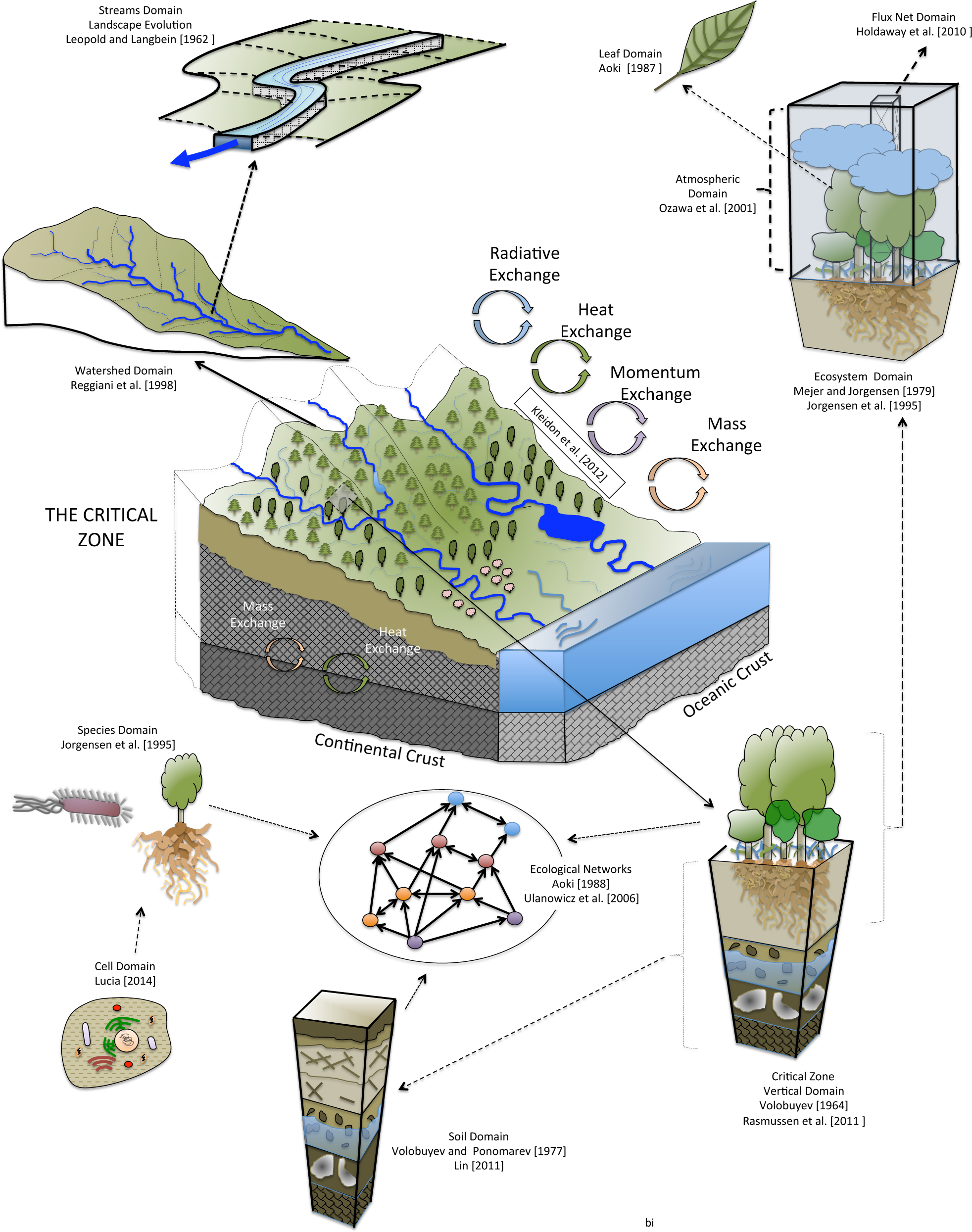
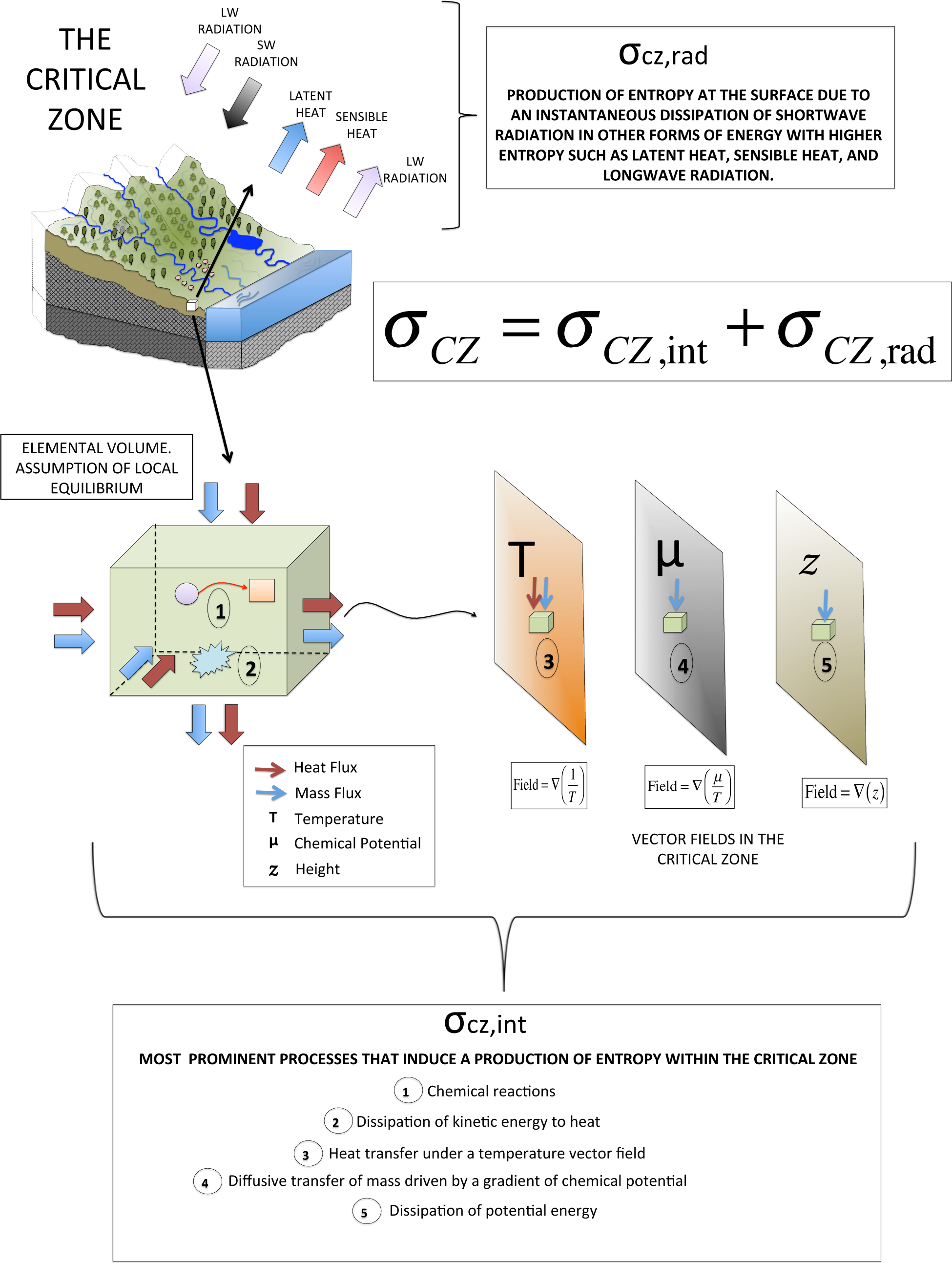
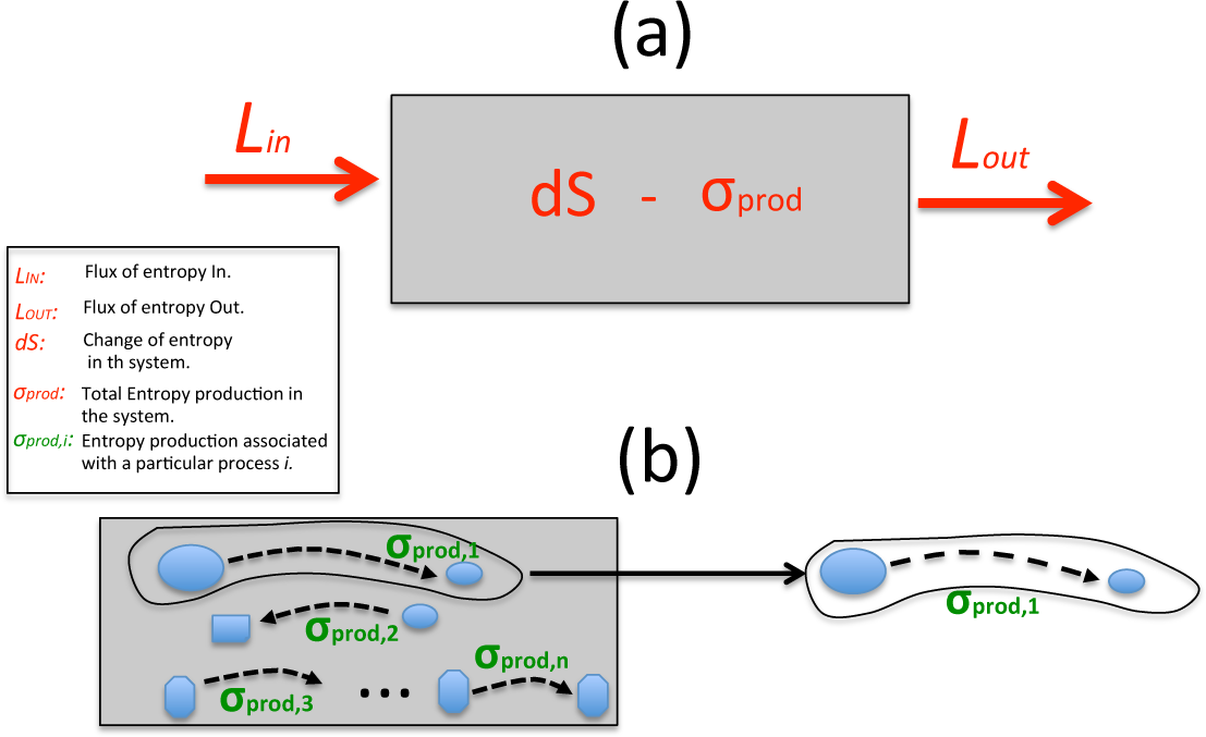
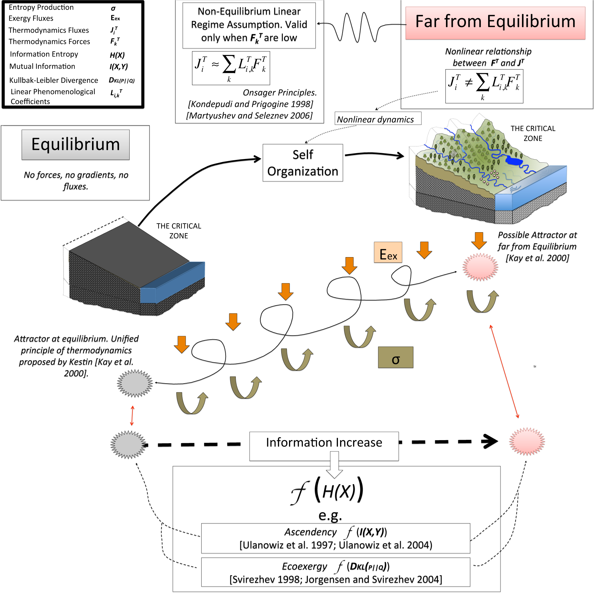
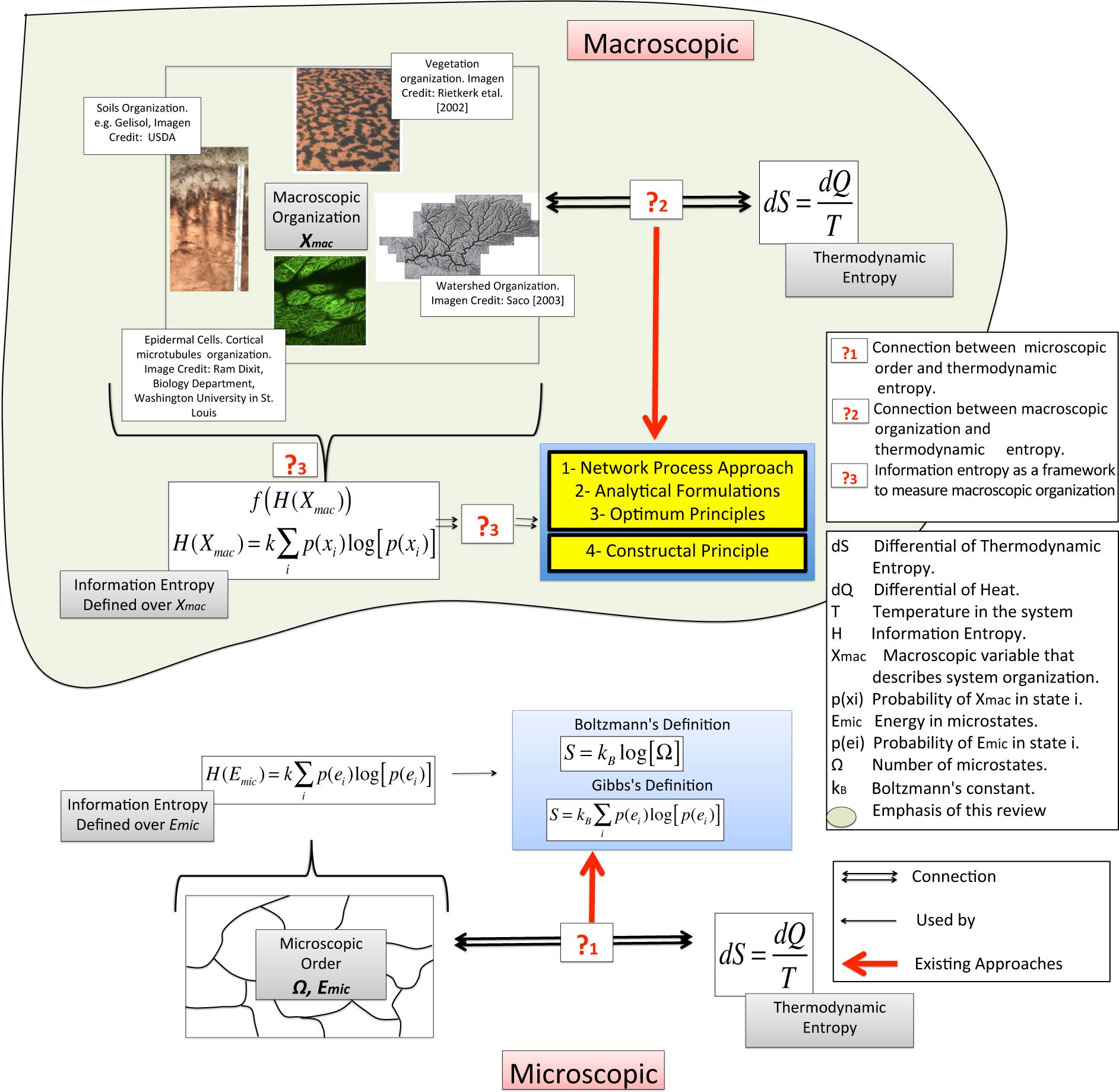
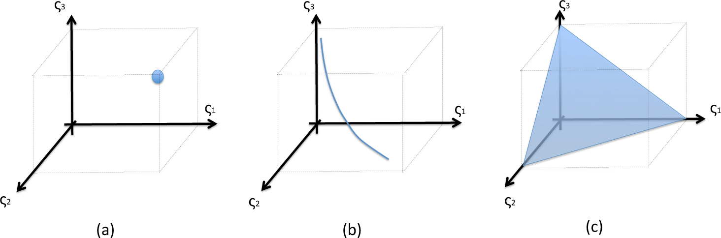
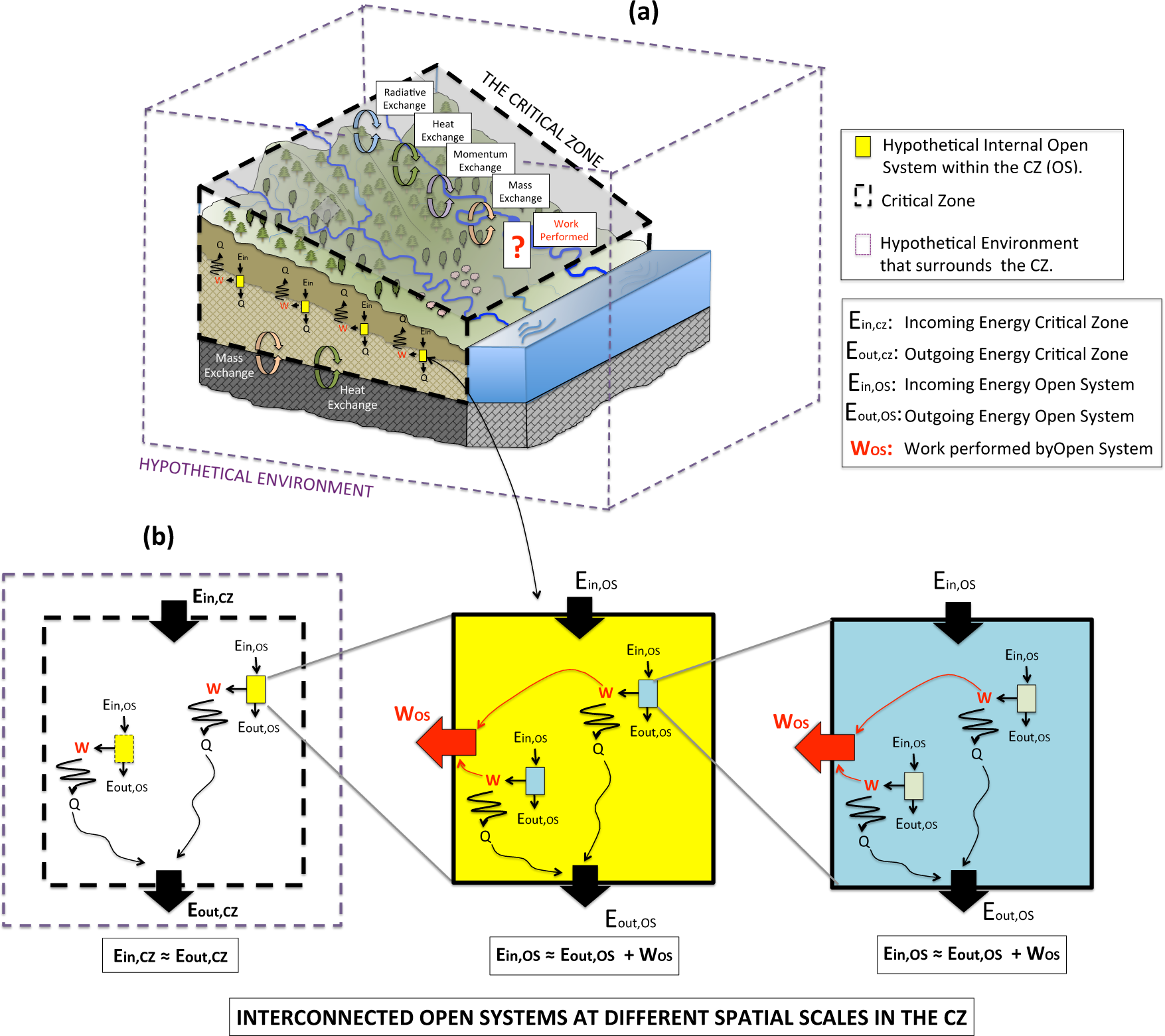
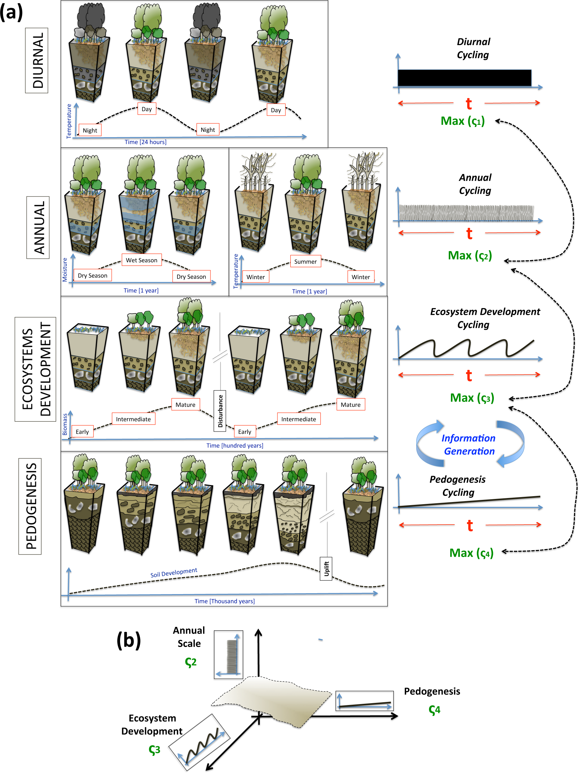
| Description | Formulation | Notations |
|---|---|---|
| (I) Entropy Flux Across the Surface of an Elemental Volume in the Critical Zone | ||
| Heat Flux | Jq Heat Flux Ik: flux of component k Mass Lrad: Flux of entropy due to radiation k T: CZ Temperature | |
| Radiation Flux | RF: Radiation Factor* Tsource: Temperature at which radiation is emitted | |
| Mass Flux | nk Mole: number per unit volume sk: Molar entropy of component k | |
| (II) Processes Associated with Entropy Production within the Critical Zone | ||
| 1. Chemical Reactions | Af: Affinity chemical reaction υi: Velocity of reaction | |
| 2. Dissipation of Kinetic Energy | δΦ: Rate of Dissipation of kinetic energy to heat | |
| 3. Heat Transfer | uk: Internal energy in component k | |
| 4. Diffusion | Mk Molar mass in component k μk: Chemical potential in component k | |
| 5. Dissipation of Potential Energy | g: Gravity of Earth z: Height | |
*RF is explained in the Online Supplement Section 3. RF for black body radiation is (4/3).
| Concept | Description | Physical Units | Units Int. System | Original Source |
|---|---|---|---|---|
| Thermodynamic Entropy (S) | A quantity associated with irreversible dissipation of free energy [11]. The product S x T in a system is a measure of the fraction of available energy that is not useful to perform work. It has also been associated with the order of a microscopic structure in terms of the number of microstates Ω [60]. | Joules Kelvin | [59] | |
| Free Energy (G) | Fraction of available energy useful to perform work. | Energy | Joules | [61,62] |
| Work (Mechanics) | When a force displaces a body an amount dx in space [11]. | Energy | Joules | |
| Work (W) (Thermodynamics) | Work of a system over the environment is done if the sole effect on everything external to the system could have been the raising of a weight [15] * | Energy | Joules | |
| Exergy (Eex) | The maximum theoretical work that can be obtain from an overall system consisting of a system its environment as the system comes into equilibrium with the environment [15]. | Energy | Joules | [61,63] |
| Eco-exergy (Ecx) | Is the conceptualization of the exergy concept to ecosystems. It quantifies the work capacity of a given ecosystem by comparing its current state with a dead homogeneous state with no gradients (thermodynamic equilibrium) [16]. | Energy | Joules | [47–49] |
| Power (Thermodynamics) | The rate of energy transfer by work [15]. | Watts | ||
| Emergy | Embodied Energy. Available energy previously used up directly or indirectly to make a product or service. In ecology it is the energy required for the formation of organisms in different trophic levels and radiation equivalent that are used | Energy | EmJoules | [55] |
| Empower | Total emergy flowing through a system over a unit time | [64] |
*In thermodynamics work is considered as a mechanism of transfer of useful energy. The definition of work in thermodynamics is more broad than the definition in mechanics.
| Application | Field | Description | Reference |
|---|---|---|---|
| Shannon Entropy H(X) | |||
| Diversity | Ecology | Used as an index to quantify the species diversity. | [69] |
| Networks | Ecology | As a measure of the stability of the network. | [70,108] |
| Time Series | Hydrology | To characterize uncertainty of hydrologic data | [78] |
| Time Series | Hydrology | As a measure of complexity in hydrological variables | [79] |
| Time Series | Hydrology | To quantify the probabilistic distribution of variables | [74,76,80] |
| Modeling | Hydrology | To analyze hydrological networks | [81] |
| Networks | Hydrology | As a different formulation to model hydrological processes | [82–84] |
| Joint Entropy H(X,Y) | |||
| Networks | Ecology | Claimed to be a measure of total flow diversity in a network | [85] |
| Mutual Information I(X,Y) | |||
| Networks | Ecology | The amount from the diversity H(X, Y) that is encumbered by structural constraints [96]. It is a primary property of a developing network [85], and the base to compute ascendency. | [109] |
| Modeling | Hydrology | To validate model predictions. | [78] |
| Time and Spatial Series | Hydrology | To analyze the uncertainty of different variables using time or spatial data. | [110,111] |
| Time and Spatial Series | Hydrology | To analyze the nonlinear dependencies between different hydrological variables. | [92,99] |
| Directional Information Transfer DITXY | |||
| Networks | Hydrology | Measure of information transfer between nodes in a network. | [92] |
| Kullback–Leibler Divergence DKL(p||q) | |||
| Networks | Ecology | Difference in the distribution between a priori and posteriori fluxes in networks | [98] |
| Networks | Ecology | To quantify eco-exergy based on the difference between the distribution of biomass at two stages of ecosystem development. | [112] |
| Conditional Uncertainty | |||
| Networks | Ecology | A measure of the amount of choice pertaining to both the inputs and outputs of an average node in the network. [85] | [85] |
| Transfer Entropy TEY→X | |||
| Networks | Ecohydrology | Measure of information flow between ecohydrological variables | [106] |
| Concept | Symbol | Symmetric | Concept | Source |
|---|---|---|---|---|
| Shannon Entropy | H(X) | A measure of uncertainty about a random variable X. | [69] | |
| Relative Shannon Entropy | HR(X) | Normalized measure of Shannon entropy.△ | ||
| Joint Entropy | H(X,Y) | Yes | A measure of uncertainty about random variables X and Y. | [69] |
| Conditional Entropy Non-Symmetric overhead (Φn) | H(X|Y) | No | A measure of uncertainty about random variable X once Y is known. | [69] |
| Mutual Information | I(X,Y) | Yes | Reduction in the uncertainty of X due to knowledge of Y. | [85] |
| Conditional Uncertainty Symmetric Overhead (Φs) | H(X,Y)−I(X,Y) | Yes | Remaining flexibility or amount of choice associated with inputs and outputs in a network | [86] |
| Conditional Mutual Information | I(X; Y|Z) | Reduction in the uncertainty of X due to knowledge of Y when Z is given. | [87] | |
| Kullback–Leibler Divergence | DKL(P||Q) | No | A measure of the distance between the distribution of two random variables. For instance, it gives a measure of the inefficiency of assuming that the distribution is Q when the true distribution is P [87]. | [88] |
| Directional Information Transfer | DITXY | No | A measure of the information transfered from Y to X. | * |
| Transfer Entropy | TEY→X | No | A measure of the distance from the hypothesis that the dynamics of X can be described entirely by its own past and no information is gained considering the dynamics of Y [90]. | [89] |
△ Introduced in 1970 by C. H. Coombsy R. Dawes, and A. Tversky [91,92].
| Optimum Principle | Description | Math. Formulation | Original Source and Discipline |
|---|---|---|---|
| - Least Work | FLUVIAL GEOMORPHOLOGY [65] | ||
| - Minimum Energy Degradation Rate | FLUVIAL GEOMORPHOLOGY [122] | ||
| - Least Rate of Energy Expenditure | • During evolution towards equilibrium conditions a natural stream chooses its course of flow in such a manner that the rate of potential energy expenditure per unit mass is maximum. | [66] FLUVIAL GEOMORPHOLOGY | |
| - Minimum Unit Stream Power | [123,124] FLUVIAL GEOMORPHOLOGY | ||
| - Minimum Stream Power | [125] FLUVIAL GEOMORPHOLOGY | ||
| - Minimum Energy Dissipation Rate | • A system is in an equilibirium condition when its rate of energy dissipation is at its minimum value. [128] | [126,127] FLUVIAL GEOMORPHOLOGY | |
| - Minimum entropy Production (MinEnt) | • In the linear regime, the total production in a system subject to flow of energy and matter reaches a minimum value at the nonequilibirum stationary state | [45] ECOLOGY FLUVIAL GEOMORPHOLOGY HYDROLOGY | |
| - Maximum Energy Flow | • Natural selection tends to make the energy flux trough the system a maximum, so far with the constraints in which the system is subject. | [4] BIOGEOCHEMISTRY ECOLOGY | |
| - Maximum Power Output | • Systems perform at an optimum efficiency for maximum power output, which is always less than the maximum efficiency. | [54] BIOGEOCHEMISTRY ECOLOGY | |
| - Maximum Emergy | • Systems that will prevail in competition with others develop the most useful work with inflowing emergy sources by reinforcing productive processes and overcoming limitations through system organization. [129] | [55] BIOGEOCHEMISTRY ECOLOGY | |
| - Maximum Empower | • In the competition among self-organizing processes, network designs that maximize empower will prevail | [64] ECOLOGY BIOGEOCHEMISTRY | |
| -Maximum Exergy Storage | • open systems has the propensity to select the organization that gives the system as much storage exergy as possible | [48] ECOLOGY BIOGEOCHEMISTRY | |
| - Principle of Maximum Entropy Production (MEPP) | • A non-equilibrium system develops so as to maximize its entropy production under present constraints [114] | [130,131] HYDROLOGY, ECOLOGY | |
| - Maximum Exergy Dissipation | • As an ecosystem develops it becomes more efficient in capturing and dissipating the exergy of incoming solar radiation | [115] ECOLOGY | |
| - Maximum Ascendency | • In the absence of major perturbations ecosystems exhibit a tendency to increase in ascendency | [109,132] ECOLOGY | |
| - Principle of Maximum Entropy (POME) | • When making inferences based on incomplete information, the probability distribution to be drawn must have the maximum entropy permitted by the available information expressed in the form of constraints [76] | [133] HYDROLOGY | |
| - Principle of Minimum Cross Entropy (POMCE) | • When making inference based on incomplete information and knowing that the data follows a reference Q distribution then the distribution P to be drawn must be that where the cross entropy is minimized | [88] HYDROLOGY |
Subscripts Description: (s) System storage; (T) flux throughout system; (d) Dissipation.
 |
 |
 |
| Objective Functions | Application |
|---|---|
| SPACE | |
| (1) At the Link Scale: Minimum Energy Expenditure and (2) At the Channel Scale: Equal Energy Expenditure per Unit Area and (3) At the Network Scale: Minimum Total Energy Expenditure | Rodríguez-Iturbe et al. [151] (Evolution of Stream Networks) |
| TIME | |
| (1) At Short Time Scales: Vegetation density will equilibrate with climate and soil to minimize plant water stress and (2) At Successional Time Scales: Species will generate optimal equilibrium community composition where canopy efficiency maximizes soil moisture and (3) At Pedogenesis Scale: Co-evolution of soils and vegetation. Vegetation will alter soil properties to maximize canopy density | Eagleson [210] (Ecohydrology) |
© 2014 by the authors; licensee MDPI, Basel, Switzerland This article is an open access article distributed under the terms and conditions of the Creative Commons Attribution license (http://creativecommons.org/licenses/by/3.0/).
Share and Cite
Quijano, J.; Lin, H. Entropy in the Critical Zone: A Comprehensive Review. Entropy 2014, 16, 3482-3536. https://doi.org/10.3390/e16063482
Quijano J, Lin H. Entropy in the Critical Zone: A Comprehensive Review. Entropy. 2014; 16(6):3482-3536. https://doi.org/10.3390/e16063482
Chicago/Turabian StyleQuijano, Juan, and Henry Lin. 2014. "Entropy in the Critical Zone: A Comprehensive Review" Entropy 16, no. 6: 3482-3536. https://doi.org/10.3390/e16063482