“Lagrangian Temperature”: Derivation and Physical Meaning for Systems Described by Kappa Distributions

Abstract

The paper studies the “Lagrangian temperature” defined through the entropy maximization in the canonical ensemble, which is the negative inverse Lagrangian multiplier corresponding to the constraint of internal energy. The Lagrangian temperature is derived for systems out of thermal equilibrium described by kappa distributions such as space plasmas. The physical meaning of temperature is manifested by the equivalency of two different definitions, that is, through Maxwell’s kinetic theory and Clausius’ thermodynamics. The equivalency of the two definitions is true either for systems at thermal equilibrium described by Maxwell distributions or for systems out of thermal equilibrium described by kappa distributions, and gives the meaning of the actual temperature, that is, the real or measured temperature. However, the third definition, that of the Lagrangian temperature, coincides with the primary two definitions only at thermal equilibrium, and thus, in the general case of systems out of thermal equilibrium, it does not represent the actual temperature, but it is rather a function of this. The paper derives and examines the exact expression and physical meaning of the Lagrangian temperature, showing that it has essentially different content to what is commonly thought. This is achieved by: (i) maximizing the entropy in the continuous description of energy within the general framework of non-extensive statistical mechanics, (ii) using the concept of the “N-particle” kappa distribution, which is governed by a special kappa index that is invariant of the degrees of freedom and the number of particles, and (iii) determining the appropriate scales of length and speed involved in the phase-space microstates. Finally, the paper demonstrates the behavior of the Lagrangian against the actual temperature in various datasets of space plasmas.

PACS Codes: 05.20.-y (Classical Statistical Mechanics); 05.20.Dd (Kinetic theory); 94.05.-a (Space plasma physics)

1. Introduction

Numerous independent developments in space plasma physics have revealed the peculiar statistical behavior of this typical category of plasmas: particle populations of space plasmas reside in stationary distributions that are out of thermal equilibrium. Thermal equilibrium is a special stationary state; systems at thermal equilibrium have their distribution function of particle velocities stabilized into a Maxwell distribution, which is connected with the classical framework of Boltzmann-Gibbs statistical mechanics. However, Maxwell distributions are extremely rare in space plasmas. The vast majority of space plasmas reside at stationary states out of thermal equilibrium, described by kappa distributions, which belong to a broader statistical framework. The kappa index that governs these distributions characterizes and distinguishes these non-equilibrium stationary states (cf. Figure 2 in [1]).

Kappa distributions have successfully described plasmas in numerous locations, including: (1) the inner heliosphere, e.g., solar wind (e.g., [1–8]), and planetary magnetospheres (e.g., [9–17]), (2) the outer heliosphere and the inner heliosheath (e.g., [18–27]), and (3) other various plasma-related analyses (e.g., [28–48]). Kappa distributions are non-Maxwellian and thus cannot embody Boltzmann-Gibbs statistical mechanics, but instead, must be described within the generalized statistical framework of non-extensive statistical mechanics that offers a solid theoretical basis for describing particle systems like space plasmas in non-equilibrium stationary states (e.g., see [49–52] and [1,34]).

Non-extensive statistical mechanics generalizes the classical framework of Boltzmann-Gibbs standing on two bases, that is (i) the Tsallis formulation of entropy parameterized by the q-index [49], and (ii) the duality of probability distributions, that is given by the ordinary p(ɛ) and escort P(ɛ)^q probability distributions of energy ɛ, related by P(ɛ)~p(ɛ)^q (normalized accordingly) [52]. The respective generalization of the Maxwellian distribution of velocities is derived by maximizing the Tsallis entropy (under the constraints of Canonical Ensemble [34]). The generalized distribution is a q-exponential function (see [34] and references therein). Such q-exponential distributions are observed quite frequently in nature and it is now widely accepted that these distributions constitute a suitable generalization of the Boltzmann-Gibbs exponential distribution. (For applications of q-exponential distributions, see [50,34] and refs therein.) [34] showed that the q-exponential distribution coincides precisely with the kappa distribution and that the entropic index q that characterizes the Tsallis entropy [49], is related to the κ-index of the kappa distribution by q = 1 + 1/κ [34]. Therefore, the q-exponential distribution is expressed in terms of the q-index and is widely used in the Statistical Physics community, while its equivalent, the kappa distribution, is expressed in terms of the κ-index and is more commonly used in the Space Physics community. The kappa distribution for a 3-dimensional system is given by the escort distribution [1,34,36],

$$P(\varepsilon )~{\left(1+\frac{1}{\kappa -\frac{3}{2}}·\frac{\varepsilon }{k_{\text{B}}T}\right)}^{-\kappa -1}$$

(1)

(k_B is the Boltzmann constant), while the respective ordinary probability distribution is:

$$p(\varepsilon )~{\left(1+\frac{1}{\kappa -\frac{3}{2}}·\frac{\varepsilon }{k_{\text{B}}T}\right)}^{-\kappa }$$

(2)

The ordinary distribution can be rewritten using the “deformed exponential” function, that is:

$${\text{exp}}_q(x)\equiv {[1+(1-q)·x]}_{+}^{\frac{1}{1-q}}\mathrm{\hspace{0.17em} }\text{or\hspace{0.28em}}{\text{exp}}_{\kappa }(x)\equiv {(1-x/\kappa )}_{+}^{-\kappa }$$

(3)

which recovers to the exponential function for q→1, or, κ→∞. (The subscript “+” denotes the cut-off condition [y]₊ = y, if y ≥ 0 and [y]₊ = 0, if y ≤ 0, [50]). Indeed, Equation (2) becomes:

$$p(\varepsilon )~{\left[1+\frac{1}{\kappa }·\frac{\varepsilon }{k_{\text{B}}T(\kappa -\frac{3}{2})/\kappa }\right]}^{-\kappa }={\text{exp}}_{\kappa }\hspace{0.17em}\left(-\frac{\varepsilon }{k_{\text{B}}{\tilde{T}}_{\text{mx}}}\right)$$

(4)

Thus, the ordinary distribution is expressed using the formulation of the deformed exponential, and naturally recovers to the classical Boltzmann-Gibbs distribution, p(ɛ) ~ exp[−ɛ/(k_BT̃_mx)], for κ→∞. However, the included temperature T̃_mx does not constitute the actual temperature T (that is the real or measure one), but some function of the actual temperature T and the kappa index κ, T̃_mx = T̃_mx (T;κ), that is:

$${\tilde{T}}_{\text{mx}}=\frac{\kappa -\frac{3}{2}}{\kappa }·T$$

(5)

This is usually called “Maxwellian temperature”. It is a function of the actual temperature T coinciding with T only at thermal equilibrium.

It is generally thought that the Maxwellian temperature T̃_mx is defined and determined by the temperature that the system would have if it was residing at thermal equilibrium and described by a Maxwell distribution (e.g., see [20,27,30,53]). However, such a definition is inconsistent:

First, both the following limits at κ→∞ lead to the same exponential function,

$${\tilde{T}}_{\text{mx}}=\frac{\kappa -\frac{3}{2}}{\kappa }·T\Rightarrow \underset{\kappa \to \infty }{\text{lim}}\hspace{0.17em}{\left(1+\frac{1}{\kappa -\frac{3}{2}}·\frac{\varepsilon }{k_{\text{B}}T}\right)}^{-\kappa }=\text{exp\hspace{0.17em}}\left(-\frac{\varepsilon }{k_{\text{B}}{\tilde{T}}_{\text{mx}}}\right)$$

(6)

$${\tilde{T}}_{\text{mx}}=T\Rightarrow \underset{\kappa \to \infty }{\text{lim}}\hspace{0.17em}{\left(1+\frac{1}{\kappa -\frac{3}{2}}·\frac{\varepsilon }{k_{\text{B}}T}\right)}^{-\kappa }=\text{exp\hspace{0.17em}}\left(-\frac{\varepsilon }{k_{\text{B}}{\tilde{T}}_{\text{mx}}}\right)$$

(7)

In fact, it could be equivalently meaningful to define the Maxwellian temperature through any general function g(κ) that becomes ~1 at thermal equilibrium, $\underset{\kappa \to \infty }{\text{lim}}g(\kappa )=1$, namely:

$${\tilde{T}}_{\text{mx}}=g(\kappa )·T\Rightarrow \underset{\kappa \to \infty }{\text{lim}}\hspace{0.17em}{\left(1+\frac{1}{\kappa -\frac{3}{2}}·\frac{\varepsilon }{k_{\text{B}}T}\right)}^{-\kappa }=\underset{\kappa \to \infty }{\text{lim}}\hspace{0.17em}{\left(1+\frac{g(\kappa )}{\kappa -\frac{3}{2}}·\frac{\varepsilon }{k_{\text{B}}{\tilde{T}}_{\text{mx}}}\right)}^{-\kappa }=\text{exp\hspace{0.17em}}\left(-\frac{\varepsilon }{k_{\text{B}}{\tilde{T}}_{\text{mx}}}\right)$$

(8)

The concept of temperature at thermal equilibrium could not be dependent on an arbitrary function g(κ) whose limit is 1, so that the limit of the kappa distribution to be exp(−ɛ/k_BT).

Second, the temperature of the system is independent of the value of the kappa index. Namely, the temperature remains constant when varying the kappa index, even when the kappa index is infinite and the kappa distribution recovers to the Maxwell distribution. Thus, statements such as “the temperature that the system would have if it was described by a Maxwell instead of a kappa distribution” are rather mistaken, because the concept and definition of temperature must be common for any kappa distribution even when this becomes a Maxwell distribution.

The expression and physical meaning of the temperature at thermal equilibrium should arise from physical concepts, and this is the main content of this paper. In particular, the two basic definitions of temperature, the kinetic and thermodynamic, are valid and equivalent either at thermal equilibrium (described by Maxwell distribution) or in stationary states out of thermal equilibrium (described by kappa distributions). These two equivalent characterizations constitute the actual temperature (the real or measured temperature). Another definition of temperature is related to the maximization of the entropy within the framework of the canonical ensemble, and leads to a well-defined temperature only at thermal equilibrium (Section 3). This constitutes the “Lagrangian temperature” and is the classical definition of temperature originated by statistical mechanics [17,34]. Similar to the Maxwellian temperature given in Equation (5), the Lagrangian temperature coincides with the actual temperature only at thermal equilibrium, while in general, it is a function of the actual temperature T and the kappa index κ.

The paper is organized as follows: Section 2 derives the canonical probability distribution by maximizing the Tsallis entropy for continuous energy states and within the framework of non-extensive Statistical Mechanics. Section 3 provides the basic definitions of temperature for systems out of thermal equilibrium described by kappa distributions. Section 4 describes the N-particle kappa distribution. Section 5 shows the analytical development of the formulation that involves the Lagrangian temperature. Section 6 derives the scale parameters that are involved in the expression of the Lagrangian temperature. Section 7 applies the theory to the proton populations of solar wind throughout the heliosphere, where the functional behavior of the Lagrangian temperature is determined. Finally, Section 8 summarizes the conclusions.

2. Derivation of the Canonical Probability Distribution

The entropy is a functional of the ordinary probability distribution in the velocity space, p(u⃗):

$$S[p(\overrightarrow{u})]=\frac{1-{\varphi }_q[p(\overrightarrow{u})]}{q-1}$$

(9)

where the argument ϕ_q is the following probability functional:

$${\varphi }_q[p(\overrightarrow{u})]\equiv {\int }_{-\infty }^{+\infty }{\left[p(\overrightarrow{u})·{{\sigma }_u}^f\right]}^q\frac{{du}_1\hspace{0.17em}{du}_2\dots {du}_f}{{{\sigma }_u}^f}$$

(10)

σ_u is the smallest speed scale parameter characteristic of the system, so that the quantity:

$$d\mathrm{\Omega }\equiv \frac{{du}_1\hspace{0.17em}{du}_2\dots {du}_f}{{{\sigma }_u}^f},$$

(11)

gives the number of microstates in the f-dimensional phase-space (see Section 5). (Note that the probability distribution p(u⃗) scales as σ_u^−f, or, p(u⃗)·σ_u^f is dimensionless.)

In the canonical ensemble, the entropy is maximized under the constraint of normalization, μ[p(u⃗)]=1, where:

$$\mu [p(\overrightarrow{u})]\equiv {\int }_{-\infty }^{+\infty }\left[p(\overrightarrow{u})·{{\sigma }_u}^f\right]\frac{{du}_1\hspace{0.17em}{du}_2\dots {du}_f}{{{\sigma }_u}^f}$$

(12)

and the constraint of the mean energy, E[p(u⃗)]=0, where:

$$E[p(\overrightarrow{u})]\equiv \frac{1}{{\varphi }_q}·{\int }_{-\infty }^{+\infty }{\left[p(\overrightarrow{u})·{{\sigma }_u}^f\right]}^q·[\varepsilon (\overrightarrow{u})-U]\frac{{du}_1\hspace{0.17em}{du}_2\dots {du}_f}{{{\sigma }_u}^f}$$

(13)

where ɛ(u⃗)=(1/2)m(u⃗−<u⃗>)² is the particle kinetic energy, and <ɛ>=(1/2)m<(u⃗−<u⃗>)²> is the particle mean kinetic energy, that is, the internal energy U in the absence of a potential energy. Given the two constraints, the entropy is maximized using the Lagrange method, that is, by using the two Lagrange multipliers λ₁ and λ₂ to maximize the constructed probability functional G[p(u⃗)] ≡ S[p(u⃗)] + λ₁·μ[p(u⃗)] + λ₂·E[p(u⃗)], i.e.:

$$\delta S=-\frac{q}{q-1}·{\int }_{-\infty }^{+\infty }{\left[p(\overrightarrow{u})·{{\sigma }_u}^f\right]}^{q-1}·\left[\delta p(\overrightarrow{u})·{{\sigma }_u}^f\right]\frac{{du}_1{du}_2\dots {du}_f}{{{\sigma }_u}^f}$$

(14)

$$\delta E\cong \frac{q}{{\varphi }_q}·{\int }_{-\infty }^{+\infty }{\left[p(\overrightarrow{u})·{{\sigma }_u}^f\right]}^{q-1}[\varepsilon (\overrightarrow{u})-U]·\left[\delta p(\overrightarrow{u})·{{\sigma }_u}^f\right]\frac{{du}_1{du}_2\dots {du}_f}{{{\sigma }_u}^f}$$

(15)

$$\delta \mu \cong {\int }_{-\infty }^{+\infty }\left[\delta p(\overrightarrow{u})·{{\sigma }_u}^f\right]\frac{{du}_1\hspace{0.17em}{du}_2\dots {du}_f}{{{\sigma }_u}^f},\hspace{0.17em}\text{hence}$$

(16)

$$\delta G=\delta S+{\lambda }_1\delta \mu +{\lambda }_2\delta E={\int }_{-\infty }^{+\infty }I(\overrightarrow{u})·\left[\delta p(\overrightarrow{u})·{{\sigma }_u}^f\right]\frac{{du}_1{du}_2\dots {du}_f}{{{\sigma }_u}^f}=0.$$

(17)

In order for the integral (17) to be zero for every fluctuating distribution p(u⃗), must I(u⃗) = 0, where:

$$I(\overrightarrow{u})\equiv {\lambda }_1-\frac{q}{q-1}·{\left[p(\overrightarrow{u})·{{\sigma }_u}^f\right]}^{q-1}·\left[1+(1-q)·{\lambda }_2·\frac{\varepsilon (\overrightarrow{u})-U}{{\phi }_q}\right]$$

(18)

The maximization leads to the Canonical probability distribution of velocities:

$$p(\overrightarrow{u})~{\left[1-(1-q)·(-{\lambda }_2)·\frac{\varepsilon (\overrightarrow{u})-U}{{\varphi }_q}\right]}^{\frac{1}{1-q}}$$

(19)

The second Lagrangian multiplier λ₂ represents the negative inverse of the Lagrangian temperature T_L, i.e., λ₂ ≡ −β_L with β_L ≡ 1/(k_BT_L), while the actual temperature T is given by β = β_L/φ_q and β = 1/(k_BT). Hence:

$$T\equiv {\varphi }_q{T}_{\text{L}}$$

(20)

The characteristic thermal speeds are $\theta \equiv \sqrt{2k_{\text{B}}T/m}$ and ${\theta }_{\text{L}}\equiv \sqrt{2k_{\text{B}}{T}_{\text{L}}/m}$. The mean kinetic energy (noted by U) is given by:

$$\langle \varepsilon \rangle =\frac{1}{2}m·\langle {(\overrightarrow{u}-<\overrightarrow{u}>)}^2\rangle =\frac{f}{2}{k}_{\text{B}}T\mathrm{\hspace{0.17em} }\text{or\hspace{0.28em}}\langle {(\overrightarrow{u}-<\overrightarrow{u}>)}^2\rangle =\frac{f}{2}·{\theta }^2$$

(21)

and thus, the ordinary p(u⃗) and escort P(u⃗) distribution functions are written as:

$$p~{\left[1+(q-1)·\frac{\varepsilon (\overrightarrow{u})-U}{k_{B}T}\right]}^{\frac{1}{1-q}},\hspace{0.17em}P~{\left[1+(q-1)·\frac{\varepsilon (\overrightarrow{u})-U}{k_{B}T}\right]}^{\frac{q}{1-q}}$$

(22)

The escort distribution P(u⃗) generalizes the classical Maxwell distribution, and is called q-Maxwellian distribution. Using the notion of kappa index, κ = 1/(q−1), the q-Maxwell distribution is transformed to its equivalent, the so-called kappa distribution, written in terms of energy or velocities as:

$$P~{\left[1+\frac{1}{\kappa -\frac{f}{2}}·\frac{\varepsilon }{k_{B}T}\right]}^{-\kappa -1}~{\left[1+\frac{1}{\kappa -\frac{f}{2}}·\frac{{(\overrightarrow{u}-{\overrightarrow{u}}_b)}^2}{{\theta }^2}\right]}^{-\kappa -1}$$

(23)

where the average particle velocity represents the bulk speed of the flow of particles, u⃗_b ≡ <u⃗>.

The physical meaning of the kappa index can be given by the reciprocal correlation coefficient of the energies of any two correlated kinetic degrees of freedom. In particular, the correlation coefficient equals to ρ = (d/2)/(κ₀+d/2) [36]: The known kappa index κ is dependent on the correlated degrees of freedom f, and can be related to an invariant kappa index κ₀ by κ(f) = κ₀ + (1/2)f. If N_C is the number of correlated particles and d is the number of degrees of freedom per particle, then f = d·N_C, and the dependent kappa index is κ(N_C) = κ₀ + (d/2)N_C. Note that κ₀ is the actual kappa index that characterizes a stationary state, and it is invariant from the number of particles and degrees of freedom of the system [36]. The “thermalization” of the system—the system to reach thermal equilibrium—is realized for quite large values of the kappa index, i.e., 1 ≪ N_C ≪ κ₀ → ∞, that is to approach infinity and the distribution to become Maxwellian. 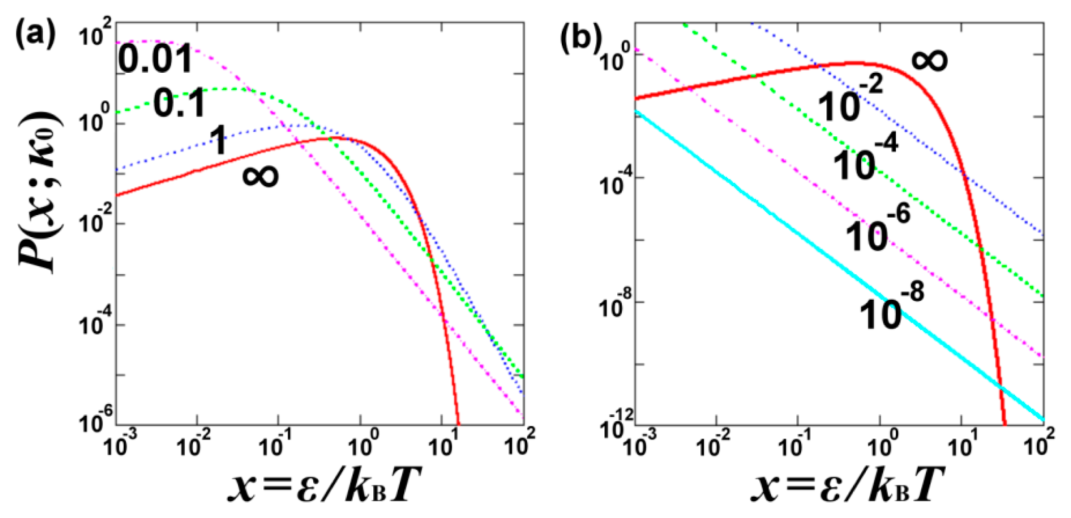Using the invariant kappa index κ₀, the kappa distribution is written as:

$$P~{\left[1+\frac{1}{{\kappa }_0}·\frac{\varepsilon }{k_{\text{B}}T}\right]}^{-{\kappa }_0-1-\frac{f}{2}}~{\left[1+\frac{1}{{\kappa }_0}·\frac{{(\overrightarrow{u}-{\overrightarrow{u}}_b)}^2}{{\theta }^2}\right]}^{-{\kappa }_0-1-\frac{f}{2}}$$

(24)

Figure 1 shows the kappa distribution of energy ɛ/(k_BT), for f = 3 degrees of freedom, and various values of the kappa index. As the kappa index increases, the maximum of the distribution lowers, while the two “edges” (for small and large x) raise, so that the mean value of x (mean energy) to be preserved. Indeed, the mean kinetic energy does not depend on the kappa index, thus, it remains constant under variations of the kappa index (kinetic definition of temperature—see Section 3).

3. Kinetic/Thermodynamic Definitions of Temperature for Systems out of Thermal Equilibrium

The temperature is a well-understood concept for particle systems at thermal equilibrium. This is based on the equivalency of the two fundamental definitions of temperature, that is (1) the kinetic definition of Maxwell (1866) [54] and (2) the thermodynamic definition of Clausius (1862) [55].

According to the Maxwell’s kinetic theory [54], the mean kinetic energy provides the kinetic definition of temperature, <ɛ> ≡ (f/2)k_BT. This is the equipartition theorem applied to each of the (f) kinetic degrees of freedom of a particle system at thermal equilibrium. In other words, the mean kinetic energy per (half) degrees of freedom defines the kinetic energy k_BT, or, the temperature (in units of J/k_B). The temperature must be independent of other thermodynamic parameters, e.g., the kappa index. Indeed, the kinetic definition of temperature is applicable for both systems at or out of thermal equilibrium, and the equipartition theorem is identical for any kappa index [1,17,34]. While the mean kinetic energy defines the temperature, the correlations between the individual particle energies define the kappa index κ₀ [36]. In principle, the kappa index and temperature are independent thermodynamic parameters, meaning that the mean kinetic energy has no effect on the particle correlations. As it was correctly stated in [32], “… clearly, from the definition of temperature, all distributions with the same mean energy per particle have the same temperature”. It is worth noting that only the second statistical moment of velocities has this fundamental physical meaning of defining temperature, and thus, no other moment is independent of the kappa index. It can be shown that the α^th moment, μ ≡ <x^α/2>^1/α (with x ≡ ɛ/(k_BT) = (u⃗−u⃗_b)²/θ²), is $\mu {(\alpha ;{\kappa }_0)}^{\alpha }\equiv {{\kappa }_0}^{\frac{\alpha }{2}}·\mathrm{\Gamma }({\kappa }_0+1-\frac{\alpha }{2})/\mathrm{\Gamma }({\kappa }_0+1)$. Figure 2 demonstrates the derivative of the α^th statistical moment with respect to the invariant kappa index κ₀, showing that only the moments for α = 0 and α = 2 are independent of the kappa index.

The thermodynamic definition of temperature is given by the connection of entropy S with the internal energy U, i.e., T ≡ (∂S/∂U)⁻¹ [55]; in the absence of a potential energy, the internal energy is given by the mean kinetic energy, i.e., the temperature. At thermal equilibrium, the two temperature definitions are equivalent, namely, they lead to the same temperature, $T\equiv {(\partial S/\partial U)}^{-1}=\frac{2}{f\hspace{0.17em}{k}_{\text{B}}}·<\varepsilon >$.

For systems out of thermal equilibrium that are described by kappa distributions, the thermodynamic definition of temperature is given by T ≡ (∂S/∂U)⁻¹·[1−(1/κ)·S/k_B]. [56] showed that this is the most generalized formulation of the temperature’s thermodynamic definition that can be consistent with the zero-th law of Thermodynamics. [34] showed the equivalence of these two different temperature definitions—the kinetic and thermodynamic—that produces a well-defined temperature for systems out of thermal equilibrium described by kappa distributions.

The “Lagrangian temperature” is a third definition, which is expressed through the second Lagrangian multiplier (λ₂) that corresponds to the constraint of internal energy in the Canonical Ensemble, as it is shown in Equations (16) and (17). While all three temperature definitions (kinetic, thermodynamic, Lagrangian) coincide at thermal equilibrium, they are typically different out of thermal equilibrium. In particular, for systems out of thermal equilibrium described by kappa distributions, the kinetic and thermodynamic temperature definitions are still equivalent, leading to a well-defined temperature for stationary states out of thermal equilibrium. However, the Lagrangian definition gives the actual temperature only at thermal equilibrium, while for any state other than thermal equilibrium, it behaves like a function of the actual temperature. (Note: The Lagrangian definition gives the temperature used in the formulation of Maxwell distribution of velocities. Therefore, the Lagrangian temperature can be also referred to as Maxwellian temperature—see Equation 8.)

The relation between the Lagrangian temperature T_L and the actual temperature T may not be a simple proportionality. The origin of the Lagrangian temperature is T_L = (−λ₂)⁻¹/k_B or T_L = (∂S/∂U)⁻¹ = T/[1−(1/κ)·S/k_B] = T/ϕ_q, that is Equation (20), which coincides with T at thermal equilibrium (κ→∞). The non-proportionality arises because the argument ϕ_q depends also on the temperature, ϕ_q = ϕ_q(T). This dependence is inherited by the speed scale σ_u = σ_u(T) (Section 5).

4. The N-Particle Kappa Distribution

The N-particle distributions can be reduced to 1-particle distributions, which are more convenient to handle but less accurate for describing the statistics of the system. In particular, the N_C-particle kappa distribution gives the probability of N_C correlated particles to have kinetic energies ɛ₁, ɛ₂, …, ɛ_N [1], i.e.:

$$P~{\left[1+\frac{1}{{\kappa }_0}·\frac{{\sum }_{i=1}^{N_{\text{C}}}{\varepsilon }_i}{k_{\text{B}}T}\right]}^{-{\kappa }_0-1-\frac{d}{2}{N}_{\text{C}}}~{\left[1+\frac{1}{{\kappa }_0}·\frac{{\sum }_{i=1}^{N_{\text{C}}}{({\overrightarrow{u}}_i-{\overrightarrow{u}}_b)}^2}{{\theta }^2}\right]}^{-{\kappa }_0-1-\frac{d}{2}{N}_{\text{C}}}$$

(25)

(which applies in the absence of a potential energy). Each particle has d kinetic degrees of freedom, thus all the N_C correlated particles have f = d·N_C total kinetic degrees of freedom. Each velocity vector contributes equally to the summation in Equation (25), which can be rewritten by substituting the summation on the particles with the summation on the degrees of freedom, i.e.:

$$P~{\left[1+\frac{1}{{\kappa }_0}·\frac{{\sum }_{j=1}^{d·N_{\text{C}}}{(u_j-u_{b,j})}^2}{{\theta }^2}\right]}^{-{\kappa }_0-1-\frac{d}{2}{N}_{\text{C}}}$$

(26)

where u_j and u_b,j denote components of the particle velocity and the bulk velocity of the plasma, respectively. The bulk velocity vector is identical for all the particles, so that the j-th component is the same with the mod(j, d) -th. Then, the summation ${\sum }_{j=1}^{d·N_{\text{C}}}{(u_j-u_{b,j})}^2$ can be considered as the velocity magnitude of a (f=d·N_C)-dimensional velocity vector u⃗. Hence, the N_C-particle kappa distribution is written as Equation (24), but now the kinetic degrees of freedom for the velocity vector are f = d·N_C instead of d.

One of the primary applications of the N-particle kappa distribution is for deriving the non-extensive thermodynamic parameters, such as the argument ϕ_q. In general, the formalism of non-extensive statistical mechanics is not supporting the usage of the more simplified 1-particle kappa distribution, but rather the more complicated N-particle kappa distribution.

5. Relation between the Lagrangian and Actual Temperature

First, we derive the expression of the argument ϕ_q that connects the actual temperature T with the classical temperature T_L. Then, substituting ϕ_q in Equation (20), we end up to the desired relation.

The argument ϕ_q is given in terms of a speed scale parameter σ_u, or equivalently, in terms of a dimensionless scale parameter σ = σ_u/θ. (The subscript u indicates that the constant σ_u is a scale of speed.) Then, we have:

$${\varphi }_q\equiv {\int }_{-\infty }^{+\infty }{[p(\overrightarrow{u})·{{\sigma }_u}^f]}^q\frac{{du}_1\hspace{0.17em}{du}_2\dots {du}_f}{{{\sigma }_u}^f}={{\sigma }_u}^{\frac{f}{\kappa }}·{\int }_{-\infty }^{+\infty }p{(\overrightarrow{u})}^{1+\frac{1}{\kappa }}\hspace{0.17em}{du}_1\hspace{0.17em}{du}_2\dots {du}_f$$

(27)

where the ordinary probability distribution in Equation (22) is normalized as follows:

$$p(\overrightarrow{u})={\pi }^{-\frac{f}{2}}{(\kappa -\frac{f}{2})}^{-\frac{f}{2}}\frac{\mathrm{\Gamma }(\kappa )}{\mathrm{\Gamma }(\kappa -\frac{f}{2})}·{\theta }^{-f}·{\left[1+\frac{1}{\kappa -\frac{f}{2}}·\frac{{(\overrightarrow{u}-{\overrightarrow{u}}_b)}^2}{{\theta }^2}\right]}^{-\kappa }$$

(28)

Without loss of generality we may set u⃗_b = 0, thus p(u⃗)=p(u) and:

$${\varphi }_q={{\sigma }_u}^{f/\kappa }\hspace{0.17em}B(f)·{\int }_{-\infty }^{+\infty }p{(u)}^{1+1/\kappa }\hspace{0.17em}{u}^{f-1}\hspace{0.17em}du$$

(29)

where the proportionality coefficient B(f) ≡ 2π^f/2/Γ(f/2) is the surface area of the f-dimensional sphere of unit radius. Then, by substituting p(u) to Equation (29), we obtain:

$${\varphi }_q={\sigma }^{\frac{f}{\kappa }}·\frac{\kappa -\frac{f}{2}}{\kappa }·{\left[{\pi }^{\frac{f}{2}}{(\kappa -\frac{f}{2})}^{\frac{f}{2}}\mathrm{\Gamma }(\kappa -\frac{f}{2})/\mathrm{\Gamma }(\kappa )\right]}^{-\frac{1}{\kappa }}$$

(30)

where we used the dimensionless scale parameter σ = σ_u/θ.

Another way to derive the argument ϕ_q is by using directly the escort distribution function, P(u⃗). This is more convenient method, because the distribution that describes the particles of the system and its statistical moments is the escort P(u⃗) and not the ordinary p(u⃗) distribution. The duality of ordinary/escort distributions is given by the following scheme:

$$P(\overrightarrow{u})·{{\sigma }_u}^f\equiv \frac{{\left[p(\overrightarrow{u})·{{\sigma }_u}^f\right]}^q}{{\int }_{-\infty }^{+\infty }{\left[p(\overrightarrow{u})·{{\sigma }_u}^f\right]}^q\frac{{du}_1\hspace{0.17em}{du}_2\dots {du}_f}{{{\sigma }_u}^f}}\iff p(\overrightarrow{u})·{{\sigma }_u}^f\equiv \frac{{\left[p(\overrightarrow{u})·{{\sigma }_u}^f\right]}^{\frac{1}{q}}}{{\int }_{-\infty }^{+\infty }{\left[P(\overrightarrow{u})·{{\sigma }_u}^f\right]}^{\frac{1}{q}}\frac{{du}_1\hspace{0.17em}{du}_2\dots {du}_f}{{{\sigma }_u}^f}}$$

(31)

from where we obtain that:

$${\varphi }_q\equiv {\int }_{-\infty }^{+\infty }{\left[p(\overrightarrow{u})·{{\sigma }_u}^f\right]}^q\frac{{du}_1\hspace{0.17em}{du}_2\dots {du}_f}{{{\sigma }_u}^f}={\left\{{\int }_{-\infty }^{+\infty }{\left[P(\overrightarrow{u})·{{\sigma }_u}^f\right]}^{\frac{1}{q}}\frac{{du}_1\hspace{0.17em}{du}_2\dots {du}_f}{{{\sigma }_u}^f}\right\}}^{-q}$$

(32)

or, in terms of the kappa index:

$${\varphi }_q={\left\{{\int }_{-\infty }^{+\infty }{\left[P(\overrightarrow{u})·{{\sigma }_u}^f\right]}^{\frac{\kappa }{\kappa +1}}\frac{{du}_1\hspace{0.17em}{du}_2\dots {du}_f}{{{\sigma }_u}^f}\right\}}^{-\frac{\kappa +1}{\kappa }}$$

(33)

The normalized escort distribution in Equation (23) is given by:

$$P(\overrightarrow{u})={\pi }^{-\frac{f}{2}}{(\kappa -\frac{f}{2})}^{-\frac{f}{2}}\frac{\mathrm{\Gamma }(\kappa +1)}{\mathrm{\Gamma }(\kappa -\frac{f}{2}+1)}·{\theta }^{-f}·{\left[1+\frac{1}{\kappa -\frac{f}{2}}·\frac{{(\overrightarrow{u}-{\overrightarrow{u}}_b)}^2}{{\theta }^2}\right]}^{-\kappa -1}$$

(34)

Again, we set u⃗_b = 0 for simplicity, so that P(u⃗) = P(u). Then, the argument ϕ_q, given by Equation (30), is derived by substituting P(u) into:

$${\varphi }_q={{\sigma }_u}^{f/\kappa }\hspace{0.17em}B{(f)}^{-\frac{\kappa +1}{\kappa }}·{\left\{{\int }_{-\infty }^{+\infty }P{(u)}^{\frac{\kappa }{\kappa +1}}\hspace{0.17em}{u}^{f-1}du\right\}}^{-\frac{\kappa +1}{\kappa }}$$

(35)

Having derived the argument ϕ_q, the connection between the actual temperature and the Lagrangian temperature is given by substituting Equation (30) into Equation (20), i.e.:

$$T_{\text{L}}=T·{\sigma }^{-\frac{f}{\kappa }}·\frac{\kappa }{\kappa -\frac{f}{2}}·{\left[{\pi }^{\frac{f}{2}}\hspace{0.17em}{\left(\kappa -\frac{f}{2}\right)}^{\frac{f}{2}}\mathrm{\Gamma }(\kappa -\frac{f}{2})/\mathrm{\Gamma }(\kappa )\right]}^{\frac{1}{\kappa }}$$

(36)

The kappa index depends on the correlated degrees of freedom as κ = κ₀ + (1/2)f [36]. Using the invariant kappa index, κ₀ ≡ κ − (1/2)f, Equation (30) is rewritten as:

$${\varphi }_q={\sigma }^{\frac{f}{\kappa }}·\frac{{\kappa }_0}{\kappa }·{\left[{\pi }^{\frac{f}{2}}{{\kappa }_0}^{\frac{f}{2}}\mathrm{\Gamma }({\kappa }_0)/\mathrm{\Gamma }(\kappa )\right]}^{-\frac{1}{\kappa }}\hspace{0.17em}\text{or}$$

(37)

$${\varphi }_q={\left(\frac{{\sigma }^2}{\pi \hspace{0.17em}e}\right)}^{1-\frac{{\kappa }_0}{\kappa }}·{\left[\frac{\mathrm{\Gamma }(\kappa ){(\kappa /e)}^{-\kappa }}{\mathrm{\Gamma }({\kappa }_0){({\kappa }_0/e)}^{-{\kappa }_0}}\right]}^{\frac{1}{\kappa }}$$

(38)

Given the number of correlated particles N_C and the degrees of freedom per particle d = 3, then f = 3N_C:

$${\varphi }_q={\left(\frac{{\sigma }^2}{\pi \hspace{0.17em}e}\right)}^{1-\frac{{\kappa }_0}{{\kappa }_0+\frac{3}{2}{N}_{\text{C}}}}{\left[\frac{\mathrm{\Gamma }({\kappa }_0+\frac{3}{2}{N}_{\text{C}})e^{\frac{3}{2}{N}_{\text{C}}}}{{({\kappa }_0+\frac{3}{2}{N}_{\text{C}})}^{{\kappa }_0+\frac{3}{2}{N}_{\text{C}}}\mathrm{\Gamma }({\kappa }_0){{\kappa }_0}^{-{\kappa }_0}}\right]}^{\frac{1}{{\kappa }_0+\frac{3}{2}{N}_{\text{C}}}}$$

(39)

that is approximated by:

$${\varphi }_q\cong {\left(\frac{3N_{\text{C}}}{2{\kappa }_0}\right)}^{-\frac{1}{3N_{\text{C}}}}·{\left(\frac{{\sigma }^2}{\pi \hspace{0.17em}e}\right)}^{1-\frac{2{\kappa }_0}{3N_{\text{C}}}}\cong \frac{{\sigma }^2}{\pi \hspace{0.17em}e}·\left\{1-\frac{1}{3N_{\text{C}}}\text{ln}\left[\left(\frac{3N_{\text{C}}}{2{\kappa }_0}\right)·{\left(\frac{{\sigma }^2}{\pi \hspace{0.17em}e}\right)}^{2{\kappa }_0}\right]\right\}$$

(40)

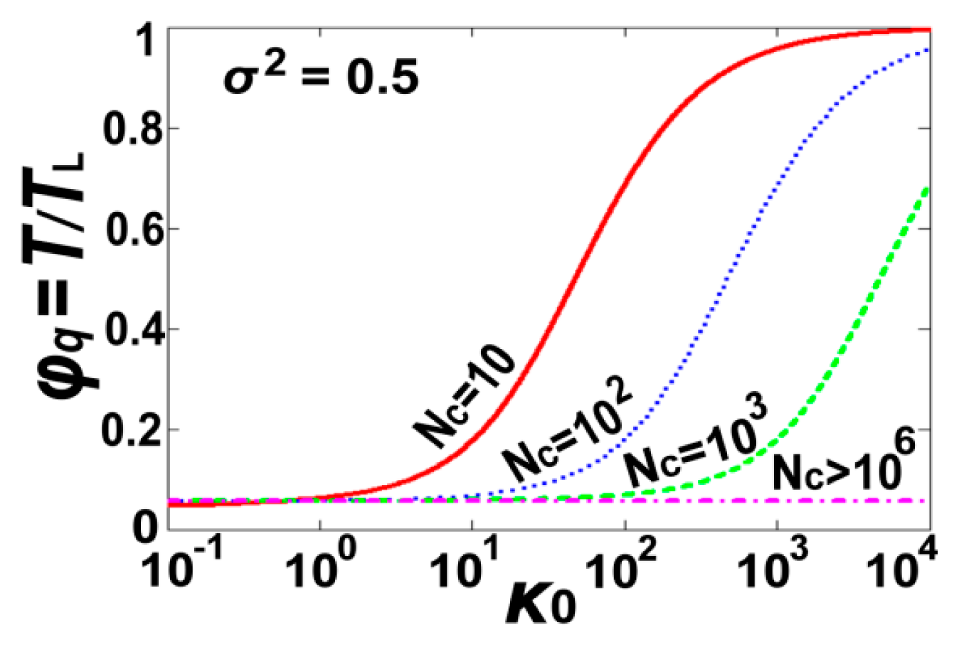
Then, the relation between the Lagrangian and actual temperature becomes:

$$T_{\text{L}}=T·{\left(\frac{\pi \hspace{0.17em}e}{{\sigma }^2}\right)}^{1-\frac{{\kappa }_0}{\kappa }}·{\left[\frac{\mathrm{\Gamma }({\kappa }_0){({\kappa }_0/e)}^{-{\kappa }_0}}{\mathrm{\Gamma }(\kappa ){(\kappa /e)}^{-\kappa }}\right]}^{\frac{1}{\kappa }}\hspace{0.17em}\text{or}$$

(41)

$$T_{\text{L}}\cong T·\frac{\pi \hspace{0.17em}e}{{\sigma }^2}·\left\{1+\frac{1}{3N_{\text{C}}}\text{ln}\left[\left(\frac{3N_{\text{C}}}{2{\kappa }_0}\right)·{\left(\frac{\pi \hspace{0.17em}e}{{\sigma }^2}\right)}^{-2{\kappa }_0}\right]\right\}$$

(42)

For large number of correlated particles, N_C≫1, the argument φ_q is ~σ²/πe, i.e., it is independent of the kappa index. Such examples are the weakly coupled plasmas; these have large number of correlation particles within Debye spheres, N_D ≡ (4π/3)nλ_D³ ≫ 1, where λ_D is the Debye length. For smaller N_C numbers, ϕ_q increases slightly with the kappa index. When the kappa index exceeds the number of particles, κ₀ > (3/2)N_C, ϕ_q increases more abruptly with the kappa index, approaching ϕ_q ~ 1. The dependence of ϕ_q on the invariant kappa index κ₀, and for various N_C, is shown in Figure 3. Next, we derive the dimensionless scale σ that can be related to the temperature, and other thermodynamic parameters, depending on the system and its correlation length.

6. The Scale Parameter

The number of microstates included in a system’s phase-space that is clustered in groups of N_C correlated particles is different from that of a classical system of uncorrelated particles (at thermal equilibrium). For classical systems, the number of microstates in an infinitesimal volume of N-particle phase-space is given by dΩ = m^3Nd⇉₁du⃗₁···d⇉_Ndu⃗_N/(N!h^3N). For systems with local correlations, the microstate number is dΩ = m^3Nd⇉₁du⃗₁···d⇉_Ndu⃗_N/(c_Nh^3N), where the combinations of correlated particles give c_N ≅ N!N_C!^N/N_C, or (c_N/N!)^1/N = N_C!^−1/N_C ≅ e/N_C.

In general, the number of microstates is written as:

$$d\mathrm{\Omega }=\frac{d^3{\overrightarrow{r}}_1{d}^3{\overrightarrow{u}}_1\cdots d^3{\overrightarrow{r}}_N{d}^3{\overrightarrow{u}}_N}{{({{\ell }_{\text{C}}}^3{\theta }^3)}^N}·{\sigma }^{-3N}$$

(43)

where the dimensionless scale parameter σ is given by:

$$\sigma \cong {(n/N_{\text{C}})}^{\frac{1}{3}}h/(m\theta )$$

(44)

with N_C ≡ (4π/3)nℓ_C³ counting the number of correlated particles. In a different approach, we can show this using the number of phase-space microstates of the correlated particles, that is:

$$d\mathrm{\Omega }=\frac{d^3{\overrightarrow{r}}_1\cdots d^3{\overrightarrow{r}}_{N_{\text{C}}}}{{{\ell }_{\text{C}}}^{3N_{\text{C}}}}·\frac{d^3{\overrightarrow{u}}_1\cdots d^3{\overrightarrow{u}}_{N_{\text{C}}}}{{{\sigma }_u}^{3N_{\text{C}}}}=\frac{d^3{\overrightarrow{r}}_1{d}^3{\overrightarrow{u}}_1\cdots d^3{\overrightarrow{r}}_{N_{\text{C}}}{d}^3{\overrightarrow{u}}_{N_{\text{C}}}}{{(h/m)}^{3N_{\text{C}}}}$$

(45)

so that:

$${\sigma }_u=\frac{h}{m{\ell }_{\text{C}}}\text{or\hspace{0.17em}}\sigma =\frac{h}{m\theta {\ell }_{\text{C}}}$$

(46)

or, given the number of correlated particles, N_C:

$$\sigma ={\left(\frac{n}{N_{\text{C}}}\right)}^{\frac{1}{3}}\frac{h}{m\theta }$$

(47)

Note that as it has been shown in [38], the presence of correlations in collisionless space plasma causes the system to be characterized on a quite large phase-space quantum, ħ_* ~10⁻²² J·s, that replaces the Planck’s constant ħ ~10⁻³⁴ J·s.

The classical case, where no correlations exist, can be considered as if the number of correlated particles were just 1, i.e., N_C ≈ 1, and the “correlation” length were reduced to the interparticle distance, ℓ_C≅b≡n^−1/3. (Precisely, it is ℓ_C = e^1/3b, for recovering the undistinguished particles combination, N!.) In this case, we have:

$$d\mathrm{\Omega }=\frac{d^3{\overrightarrow{r}}_1\cdots d^3{\overrightarrow{r}}_N}{L^{3N}}·\frac{d^3{\overrightarrow{u}}_1\cdots d^3{\overrightarrow{u}}_N}{{{\sigma }_u}^{3N}}=\frac{d^3{\overrightarrow{r}}_1{d}^3{\overrightarrow{u}}_1\cdots d^3{\overrightarrow{r}}_N{d}^3{\overrightarrow{u}}_N}{N!{(h/m)}^{3N}}$$

(48)

so that:

$${\sigma }_u=\frac{N{!}^{\frac{1}{3N}}}{L}·\frac{h}{m}\cong {\left(\frac{n}{e}\right)}^{\frac{1}{3}}\frac{h}{m}\text{or\hspace{0.17em}}\sigma \cong {\left(\frac{n}{e}\right)}^{\frac{1}{3}}\frac{h}{m\theta }$$

(49)

where we used the approximation N!≅(N/e)^N.

Different characteristic correlation lengths induce different types of relation between the Lagrangian temperature-like parameter T_L and the system’s (actual) temperature T. For κ₀ ≪ N_C→∞, all of these relations can be described by a power-law dependence, T_L~T^α, where α is hereby called thermal equilibrium index. Therefore, different correlation lengths induce different types of the exponent α. Consider the following five types of correlation lengths ℓ_C : (i) Interparticle distance, b~n^−1/3, that gives the lower limit of a correlation length, because below this limit, there is one particle the most, and thus, correlations are no effective; (ii) Debye length, ${\lambda }_{\text{D}}\propto \sqrt{T/n}$, that is the smallest length scale of local correlations in plasmas and is caused by Debye shielding electrostatic particle-particle interactions [39]; (iii) thermal wavelength, ${\lambda }_{\text{W}}~\sqrt{T}$, that is the particle thermal speed over the wave frequency, and is caused by wave-particle interactions [57]; (iv) thermal gyro-radius, ${\rho }_g~\sqrt{T}/B$, that is the ion thermal gyro-radius caused by an ambient magnetic field; (v) mean free path, L_m ~ θ/ν_col ~T²/n (ν_col: collision rate), that gives the upper limit of a correlation length; beyond the mean free path, correlations are strongly damped by collisions.

Finally,

Table 1. Lagrangian temperature for various correlation lengths.

ℓC	${\sigma }_u\propto {\ell }_{\text{C}}^{-1}$	γ = log n/logT[a]	TL∝T2ℓC2	α = log TL/logT[b]
b ~ n−1/3	n1/3	5/3	T2n−2/3	$2-\frac{2}{3}\nu =2-\frac{2}{3(\gamma -1)}$
${\lambda }_{\text{D}}\propto \sqrt{T/n}$	$\sqrt{n/T}$	3/2	T3n−1	$3-\nu =3-\frac{1}{\gamma -1}$
${\lambda }_{\text{W}}~\sqrt{T}$	$1/\sqrt{T}$	1	T3	3
${\rho }_g~\sqrt{T}/B$	$B/\sqrt{T}$	1+b[c]	T3n−2b	$3-2b\nu =3-\frac{2b}{\gamma -1}$
Lm ~ θ/νcol ~T2n−1	n/T2	7/5	T6n−2	$6-2\nu =6-\frac{2}{\gamma -1}$

^[a]Polytropic index for a constant σ;

^[b]Given a polytropic relation n ~ T^ν, γ ≡ 1+1/ν;

^[c]Given a relation of the type B ~ n^b.

shows for the limiting case κ₀ ≪ N_C → ∞, the relation between the Lagrangian temperature T_L and the actual temperature T, and gives the various values of the index α that correspond to the above five correlation lengths ℓ_C.

7. Application to the Solar Wind Throughout the Heliosphere

The presented theory is applied to the proton populations of solar wind throughout the heliosphere, that is from the inner heliosphere (some decimals of AU to ~10 AU) to the distant inner heliosheath. Equation (42) is used for deriving T_L, where the involved scale is given by Equation (46):

$$\sigma =h_{*}/(m\theta \hspace{0.17em}{\ell }_{\text{C}})=2\pi \hspace{0.17em}{\hslash }_{*}/(\sqrt{2m{k}_{\text{B}}T}{\ell }_{\text{C}}),$$

(50)

For a proton/ion single-charged plasma, this is written as:

$$\sigma =h_{*}/(\sqrt{m_i{m}_e{\theta }_i{\theta }_e}\hspace{0.17em}{\ell }_{\text{C}})=2\pi \hspace{0.17em}{\hslash }_{*}/(\sqrt{2k_{\text{B}}{m}_i{m}_e{T}_i{T}_e}{\ell }_{\text{C}})$$

(51)

Hence:

$$\sigma \cong 6^{\frac{1}{3}}{\pi }^{\frac{2}{3}}{2}^{-\frac{1}{2}}{k_{\text{B}}}^{-1}{\varepsilon }^{-\frac{1}{2}}e{(m_i{m}_e)}^{-\frac{1}{4}}{\hslash }_{*}\hspace{0.17em}{n}^{\frac{1}{2}}{(T_i{T}_e)}^{-\frac{3}{4}}{(T_i+T_e)}^{\frac{1}{2}}$$

(52)

Considering that the correlation length is the Debye length, ${\ell }_{\text{C}}={\lambda }_{\text{D}}\cong \sqrt{(k_{\text{B}}\varepsilon /{q_e}^2)T_0/n}$ , where $T_0={(T_i^{-1}+T_e^{-1})}^{-1}$ is the “effective” temperature, q_e is the elementary charge, and ɛ is the plasma permittivity; (in Figure 4 we assume T_i ≅ T_e, i.e., T₀ ≅ T_i/2).

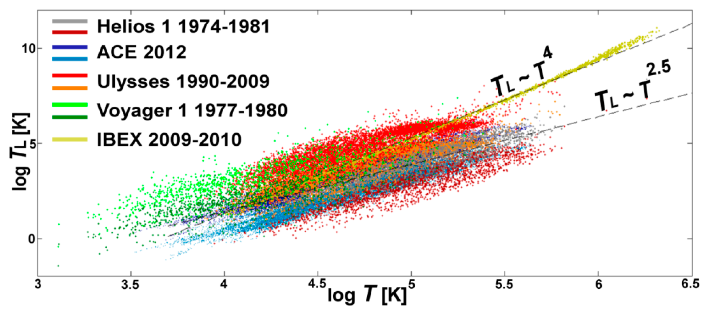
Figure 4 shows the relation between the (calculated) Lagrangian temperature T_L and the (given) actual temperature T of solar wind throughout the heliosphere. While the values of the solar wind’s temperature span a range between a few thousands to a few million degrees, the derived values of the Lagrangian temperature span a larger range from 1 K to 10¹⁰ K. For example, for T ~ 10⁴ K the Lagrangian temperature ranges from T_L ~ 1 K to T_L ~ 10⁴ K, while for T ~ 10⁵ K the Lagrangian temperature ranges from T_L ~ 10² K to T_L ~ 10⁶ K. The auxiliary line, given by log T_L ~ −8.6+2.5·logT, describes the average of the determined values of the Lagrangian temperature for the inner heliosphere (r up to 10 AU), that is for all the used datasets except IBEX. The slope (on a log-log scale) is α ~ 2.5 (see Table 1), corresponding to average polytropic index ν ~ 0.5 or γ ~ 3, that is the polytropic index that characterizes space plasmas (e.g., see [58]). The auxiliary line, given by logT_L~−14.7+4·logT, describes the average of the determined values for the inner heliosheath using the IBEX datasets [22,24,26].) In this case, the slope (on a log-log scale) is α ~ 4, corresponding to average polytropic index ν ~ −1 or γ ~ 0, that is the value of polytropic index that was found to describe the inner heliosheath [8].

8. Conclusions

The paper presented a theoretical result that has not been previously reported, the derivation of the “Lagrangian temperature” and its exact expression in terms of physical characteristics and thermodynamic parameters of the system. The Lagrangian temperature is a physical quantity, a temperature-like parameter that coincides with the actual temperature of the system only when the particles of the system reside at thermal equilibrium, while it completely differs with the temperature when the system is out of thermal equilibrium. In particular, the paper studied the behavior of the Lagrangian temperature for systems out of thermal equilibrium described by kappa distributions, such as space plasmas.

The derivation of the Lagrangian temperature was achieved by: (i) maximizing the entropy in the continuous description of energy within the general framework of non-extensive statistical mechanics, (ii) using the concept of the “N-particle” kappa distribution, which is governed by a special kappa index that is invariant of the degrees of freedom and the number of particles, and (iii) determining the appropriate scales of length and speed involved in the phase-space microstates.

The exact expression and physical meaning of the Lagrangian temperature has essentially different content to what is commonly thought. It was shown that the Lagrangian temperature is a function of the actual temperature of the system, the number of correlated particles, and a characteristic speed scale that depends on several other thermodynamic parameters.

The importance of the Lagrangian temperature is not restricted to the theoretical understanding of the concept of temperature (e.g., [56,59,60]). It has also significant merit for understanding the mixing process of systems that are out of thermal equilibrium. For example, what would be the outcome of mixing two space plasmas that are out of thermal equilibrium described by kappa distributions? The temperature follows the simple calorimetry rules when mixing two classical gases, that is, if we mix two plasmas with different temperatures and densities, the mixed-plasma would have a mass-weighted average temperature of the combined plasma [1]. However, the respective rule for the kappa indices is still unknown. Since the mean energy (i.e., the temperature) is independent of the kappa index, it cannot be used to extract the missing rule. It may be the case that the Lagrangian temperature follows the same type of rule as the actual temperature. Since the Lagrangian temperature is a function of the actual temperature and other thermodynamic parameters of the system including the kappa index. Then, any type of rules that include the Lagrangian temperature could lead to the mixing rule of kappa indices.