Feature Extraction Method of Rolling Bearing Fault Signal Based on EEMD and Cloud Model Characteristic Entropy

Abstract

The randomness and fuzziness that exist in rolling bearings when faults occur result in uncertainty in acquisition signals and reduce the accuracy of signal feature extraction. To solve this problem, this study proposes a new method in which cloud model characteristic entropy (CMCE) is set as the signal characteristic eigenvalue. This approach can overcome the disadvantages of traditional entropy complexity in parameter selection when solving uncertainty problems. First, the acoustic emission signals under normal and damage rolling bearing states collected from the experiments are decomposed via ensemble empirical mode decomposition. The mutual information method is then used to select the sensitive intrinsic mode functions that can reflect signal characteristics to reconstruct the signal and eliminate noise interference. Subsequently, CMCE is set as the eigenvalue of the reconstructed signal. Finally, through the comparison of experiments between sample entropy, root mean square and CMCE, the results show that CMCE can better represent the characteristic information of the fault signal.

1. Introduction

The rolling bearing is the most common element of the rolling mechanism. Approximately 30% of mechanical faults occur in rolling bearings; hence, detecting and diagnosing faults in rolling bearings are popular issues among scholars worldwide. In the last 10 years, acoustic emission (AE) technology has become significant in monitoring the states of rolling bearings. This technology can help effectively detect early signs of pitting corrosion defect and crack initiation, and thus, prevent disastrous consequences [1,2]. Researchers have investigated characteristic extraction methods for AE signals on bearings. A.M. Al-Ghamdi compared the root mean square (RMS), amplitude, and kurtosis values of the AE and vibration signals from the outer race fault of a rolling bearing. He asserted that AE technology was more effective than vibration technology in early fault diagnosis [3]. P. Beck investigated related parameters of AE, such as the relationship between physical properties and AE energy in material fracturing. The test results revealed a linear relationship between AE energy and fracture area or depth [4]. B. Kilundu employed a cyclostationary technique and proposed an indicator that was more sensitive to the continuous monitoring of defects compared with traditional temporal indicators (e.g., RMS, kurtosis, crest factor) [5].

Considering the poor working environment of mechanical equipment, signals collected on-the-spot are frequently seriously polluted. To eliminate noise from signals, some researchers introduced wavelet noise reduction technology into the feature extraction of AE signals and achieved good results. However, this method exhibits difficulties in selecting the wavelet base and determining the threshold. Empirical mode decomposition (EMD) does not have a fixed basis formula, and thus, difficulties in selecting wavelet base during wavelet analysis can be avoided. This technique is more effective in non-stationary signal de-noising than other wavelet transform methods. [6]. However, EMD suffers from model mixing problems, which can distort the decomposed intrinsic mode function (IMF). To solve the frequency mixing problem in EMD de-noising, Huang proposed ensemble EMD (EEMD) to perform signal decomposition and enhance the thoroughness of de-noising [7].

Given the complex structure of mechanical equipment, existing randomness and fuzziness in fault causes, fault phenomena, and fault mechanisms may result in uncertainty in signal acquisition. Uncertainty can influence the accuracy of signal feature extraction and reduce the precision of fault diagnosis. Entropy is a measurement unit of uncertainty. It can effectively reduce the dimension of an eigenvalue and fully represent the feature information of a signal. Energy entropy, information entropy, appropriate entropy (ApEn), sample entropy (SampEn), and so on, are frequently used as the eigenvalue of signals. Yan et al. [8] integrated ApEn into the state monitoring of bearings and achieved good results. Su et al. [9] introduced SampEn into fault feature extraction in rolling bearings. Based on the results of experiments, SampEn performs better than ApEn, which is suitable for distinguishing the fault states of rolling bearings. However, these two methods experience difficulty in terms of the complexity in parameter selection and other shortcomings, such as a slight variation in threshold will cause a sudden change in entropy, which affects the stability of statistics. To overcome the disadvantages of traditional entropy, this study presents a solution; namely, cloud model characteristic entropy (CMCE). CMCE (E_n) is obtained from a reverse cloud generator without threshold and dimension settings. This generator can prevent the difficulties caused by parameter selection and better solve the uncertainty problem.

Based on a cross of probability theory and fuzzy mathematic theory, Li [10] proposed that the cloud model, which was obtained from a specific structure algorithm, could be an alternative model of qualitative concepts and quantitative expressions. The cloud model cannot only reflect the uncertainty of a natural language concept, but also the correlation between randomness and fuzziness, which constitutes mutual mapping between qualitative and quantitative concepts. CMCE is one of the digital characteristics of the cloud model that can represent the uncertainty measurement of qualitative concepts. In [11], Li evaluated the stability of segmented sequence data, and then identified and expressed the basic characteristics of a time series in self-adaption. In [12], Yu used CMCE to measure the fluctuation range of harmonic current under normal operation mode. Harmonic current was determined according to the curves of the 3E_n outer boundary of normal cloud membership. Meanwhile, the cloud model is widely applied in the field of emitter identification, power transformer fault diagnosis, and network intrusion detection, among others [13,14,15]. However, the use of this model in the fault signal feature extraction of rolling bearings has not yet been reported. Accordingly, this study decomposes AE signals using the EEMD algorithm and selects sensitive IMFs that can represent characteristic information via the mutual information (MI) algorithm to eliminate noise interference. Meanwhile, CMCE is used as the eigenvalue of the reconstructed signal to overcome the shortcomings of traditional entropy. This process can improve the accuracy of signal feature extraction and the precision of fault diagnosis.

2. AE Signal Feature Extraction Theory of Rolling Bearing

2.1. EEMD Algorithm

The EEMD algorithm is an auxiliary signal processing method that deals with noises. In this algorithm, Gaussian white noise is imposed on the signals, and mixed signals are calculated repeatedly via empirical mode decomposition. After noise is added, signal continuity may be achieved in regions with different frequencies because of the evenly distributed statistical properties of Gaussian white noise frequencies. Consequently, the mixing degree of the IMF component model is reduced. The EEMD algorithm is described as follows [16].

(1)

The overall average time M and the standard deviation of white noise k are set.

(2)

The EMD experiments are performed m times after adding white noise.

(2.1)

After a random Gaussian white noise n_m(t) is added into the input signal x(t), signal x_m(t) is obtained as follows:

$$x_m(t)=x(t)+k{n}_m(t)$$

(1)

(2.2)

x_m(t) is decomposed by EMD to obtain c_j,m, which indicates that j IMF is obtained in the m-th decomposition (j = 1, 2, …, N_m). N_m denotes the number of IMF in the m-th decomposition.

(2.3)

If m < M, then let m = m + 1 and return to (2.2).

(2.4)

Take the minimum number of model components in each IMF group, which is obtained in M times decomposition as the final overall average number of IMF.

(3)

Each IMF in m times decomposition is averaged as follows:

$$\overline{X}=\frac{1}{n}{\displaystyle \sum _{i=1}^n{x}_i},\left(j=1,2,\dots ,N_m;m=1,2,\dots ,M\right)$$

(2)

(4)

${\overline{c}}_j$ is outputted as the j-th IMF obtained after EEMD decomposition. The added white noise n_m(t) is generated randomly in each experiment. When the value of M is large, the overall average of the added Gaussian white noise is close to zero.

2.2. MI Algorithm

The MI algorithm was proposed by Claude Elwood Shannon, the developer of information theory. This algorithm refers to the statistical correlation between two random variables and is obtained from the extended concept of entropy. Entropy refers to a measure of the degree of disordered state of a physical system. The variable of entropy X is defined as [17]

$$H(X)=-{\displaystyle \sum _{x\in X}p(x){\log }_{2}p(x)}$$

(3)

where p(x) is the probability that event X will occur.

Conditional entropy between two different random variables X and Y is defined as follows:

$$H(X|Y)=-{\displaystyle \sum _{x\in X,y\in Y}p(y)p(x|y){\log }_{2}p(x|y)}$$

(4)

where p(y) is the probability that event Y will occur independently, and p(x|y) is the conditional probability that event X will occur under the condition that event Y is occurring. The joint entropy of X and Y is

$$H(X,Y)=-{\displaystyle \sum _{x\in X,y\in Y}p(x,y){\log }_{2}p(x,y)}$$

(5)

where p(x, y) is the simultaneity probability (i.e., joint probability) that events X and Y will occur. In general, the relationship between the unite information entropy and the conditional information entropy is

$$H(X,Y)=H(X|Y)+H(Y)$$

(6)

For variables X and Y, the definition of MI is as follows:

$$I(X,Y)=H(X)-H(X|Y)=H(X)+H(Y)-H(X,Y)$$

(7)

The MI obtained from Equation (5) is not domesticated, and will be domesticated by Equation (6) as follows:

$$NMI=\frac{I(X,Y)}{\sqrt{H(X)\cdot H(Y)}}$$

(8)

2.3. Cloud Model Algorithm and CMCE

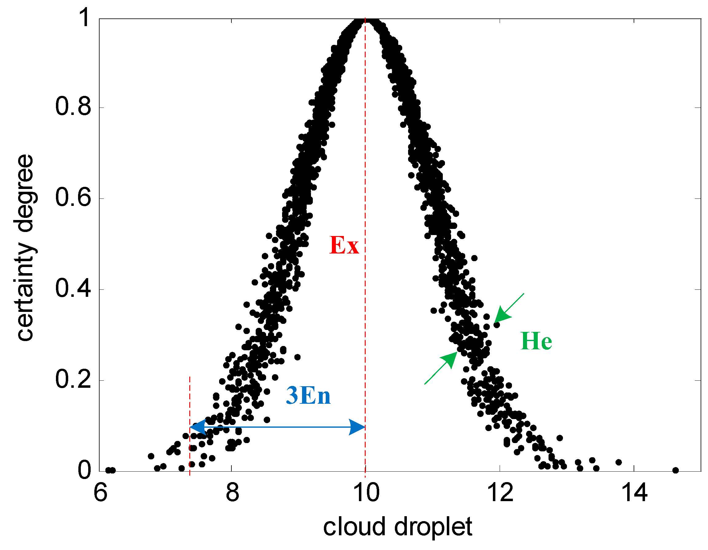
2.3.1. Cloud Model Algorithm

Let U be a quantitative universe that can be represented by a number, and C is the qualitative concept of U. If the quantitative value $x\in U$ is the first random realization of the qualitative concept C, then x’s certainty degree for C $\text{μ}(x)\in [0,1]$ is a stable tendency random number. If $\text{μ}:U\in [0,1]$, $\forall x\in U$, and x → μ(x), then the distribution of x in the universe is a cloud, which can be denoted as C(x). Each x is called a cloud droplet. The numerical characteristics of the cloud model include E_x (expected value), E_n (CMCE), and H_e (hyper entropy). The cloud model algorithm is divided into backward cloud generator algorithm and normal cloud generator algorithm [18].

The backward cloud generator algorithm indicates that a certain amount of data samples are expressed as qualitative concepts, which are expressed by digital characteristics, as shown in the following discussion.

(1)

Sample mean $\overline{X}=\frac{1}{n}{\displaystyle \sum _{i=1}^n{x}_i}$ is obtained according to sample point x_i, The first order of the sample absolute center distance is $\frac{1}{n}{\displaystyle \sum _{i=1}^n|x_i-\overline{X}|}$, and sample variance is $S^2=\frac{1}{n-1}{\displaystyle \sum _{i=1}^n{(x_i-\overline{X})}^2}$.

(2)

Calculate the expected value as follows.

$$E{}_x=\overline{X}$$

(9)

(3)

Calculate CMCE as follows.

$$E_n=\sqrt{\frac{\pi }{2}}\times \frac{1}{n}{\displaystyle \sum _{i=1}^n\left|x_i-E_x\right|}$$

(10)

(4)

Calculate hyper entropy as follows.

$$H_e=\sqrt{S^2-{E_n}^2}$$

(11)

A normal cloud generator represents a mapping from qualitative mode to quantitative mode, and the cloud droplet is obtained according to digital characteristics (E_x, E_n, H_e). This algorithm generates random quantitative values with uncertain concepts as well as the degree of certainty of random quantitative values. The steps of the normal cloud generator algorithm are described as follows.

(1)

Generate a normal random number E_n′ with expected value E_n and standard deviation H_e.

$$f_{{E^{\prime }}_n}(x)=\frac{1}{\sqrt{2\pi }{H}_e}\exp [-\frac{{(x-E_n)}^2}{2H_e^2}]$$

(12)

(2)

Generate a normal random number “x” with expected value E_x and standard deviation E_n′.

$$f_x(x)=\frac{1}{\sqrt{2\pi }\left|{E^{\prime }}_n\right|}\exp [-\frac{{(x-E_x)}^2}{2{E^{\prime }}_n^2}]$$

(13)

The probability density formula of X is

$$f_x(x)={f^{\prime }}_{E_n}(x)\times f_X(x|{E^{\prime }}_n)={\displaystyle {\int }_{-\infty }^{\infty }\frac{1}{2\pi He\left|y\right|}}\exp [-\frac{{(x-E_x)}^2}{2y^2}-\frac{{(y-E_n)}^2}{2H{e}^2}]dy$$

(14)

The expected value of cloud droplet X is E(X) = E_x, and its variance is D(X) = E_n² + H_e².

(3)

Calculate

$$y=\exp [-\frac{{(x-E_x)}^2}{2{({E^{\prime }}_n)}^2}]$$

(15)

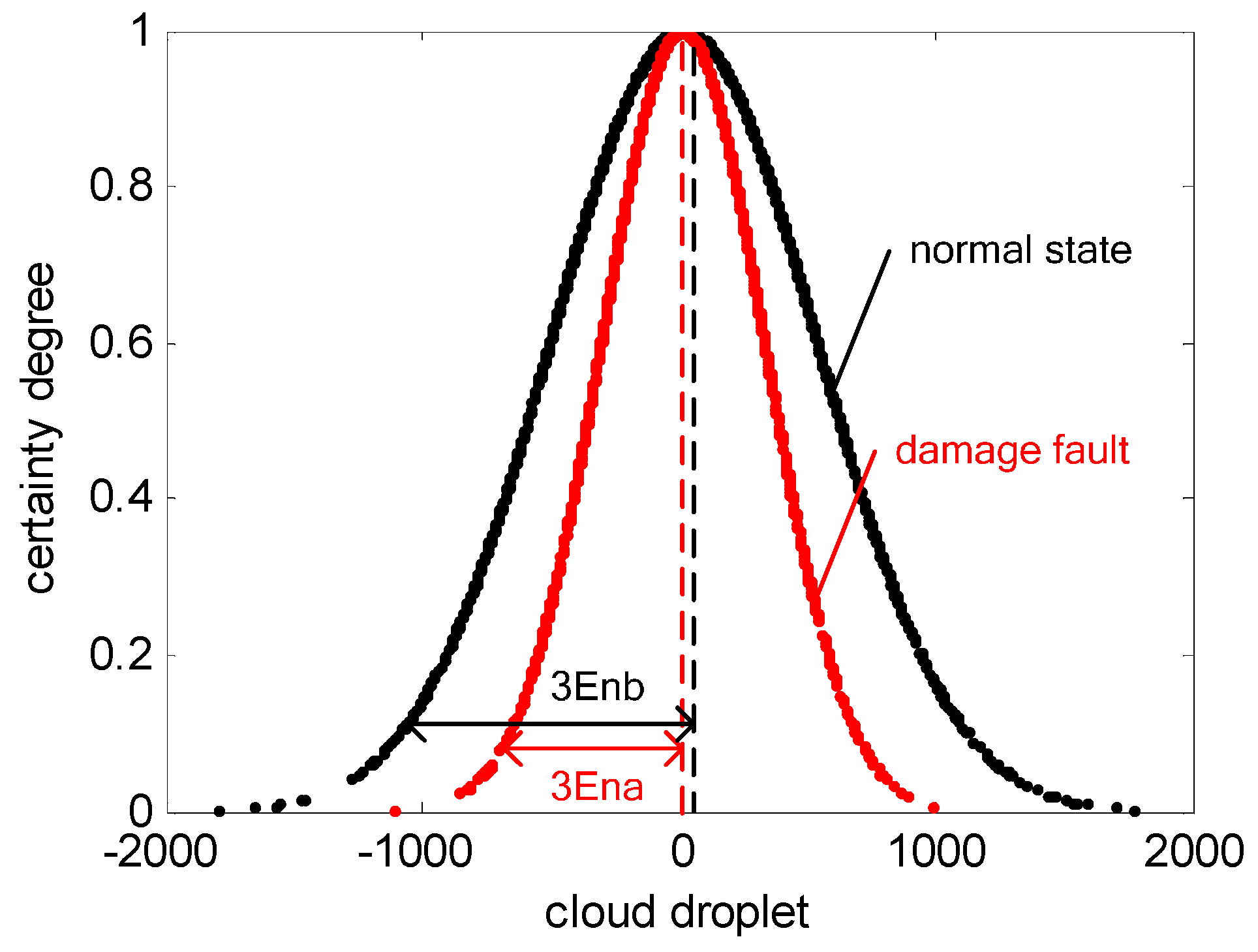
(4)

X is a cloud droplet of the universe, and y is the certainty degree.

(5)

Repeat Steps (1)–(4) until the required number of cloud droplets is generated. The schematic of the final cloud model is shown in Figure 1.

Figure 1. Schematic of the cloud model.

Figure 1. Schematic of the cloud model.

2.3.2. CMCE

All properties of the concept expressed by the cloud model can be reflected by the digital characteristics of the cloud. The cloud model uses expected value (E_x), CMCE (E_n), and hyper entropy (H_e). Overall, these three digital characteristics symbolize the same concepts C (E_x, E_n, H_e). Among these, CMCE (E_n) represents the uncertainty of the reflected qualitative concept. CMCE (E_n) indicates the range of the cloud droplet group accepted by linguistic terms in the log domain space, which is also called ambiguity. Alternatively, CMCE (E_n) denotes the randomness of the appearance of a cloud droplet; a cloud droplet can symbolize a qualitative concept. Moreover, entropy also indicates the relevance between uncertainty and randomness. CMCE (E_n) can be used to represent the particle size of a qualitative concept. In general, when entropy is high, the concept is macroscopic, fuzziness and randomness are considerable, and definite quantization is difficult.

2.4. Signal Feature Extraction Method Based on EEMD and CMCE

According to the preceding analysis, the feature extraction method based on EEMD and CMCE can be concluded through the following steps.

(1)

IMF_j (j = 1, 2, …, n) is obtained by decomposing the collected AE signals calculated by the EEMD algorithm.

(2)

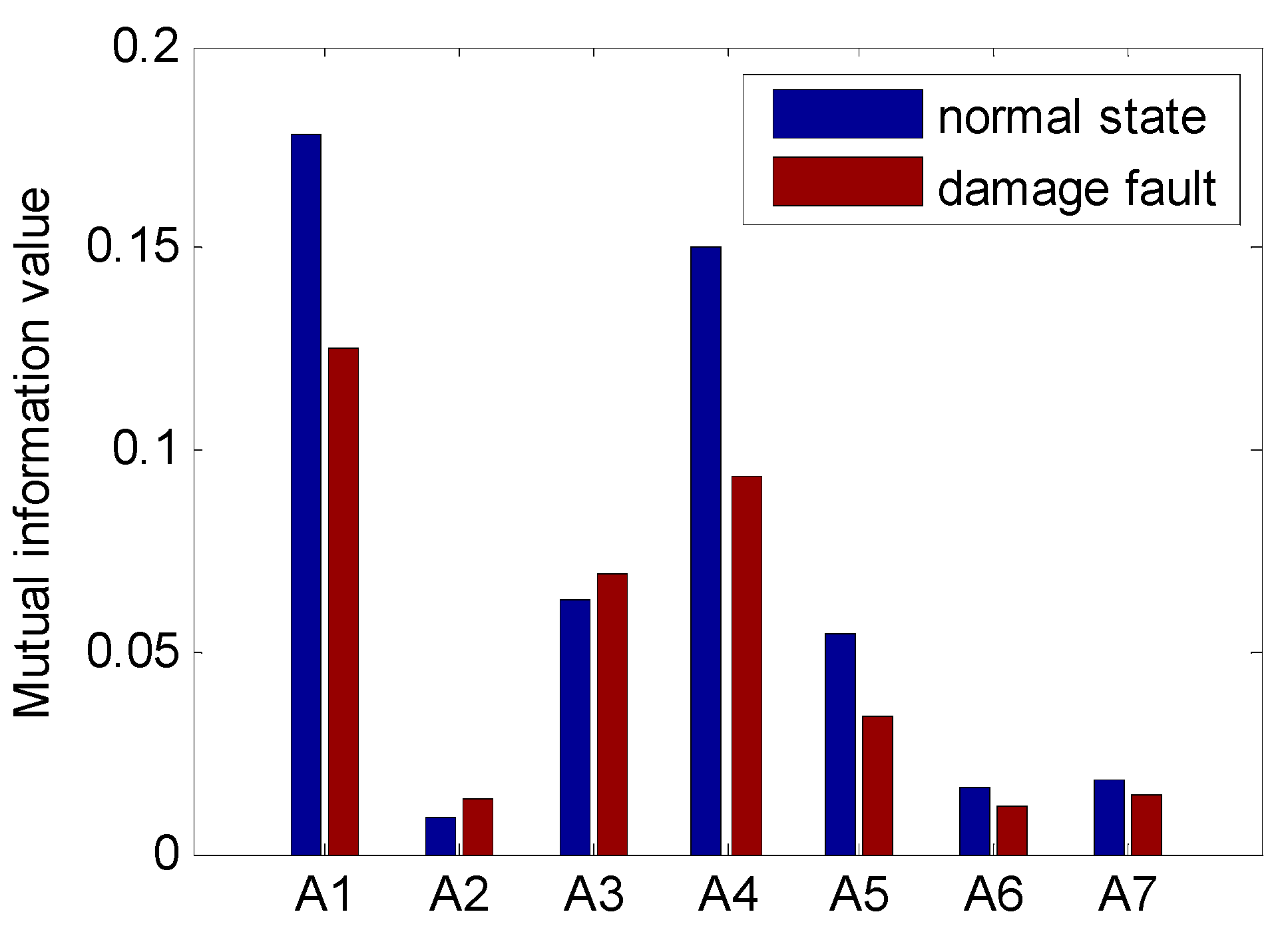
All MI values between all IMF_j and the original signal by the MI algorithm are calculated. Sensitive IMFs are selected according to MI threshold.

The formula of the MI threshold is shown as follows [19]

$${\text{μ}}_h=\frac{\max ({\mu }_i)}{10\times \max ({\mu }_i)-3}i=1,2,\dots ,n$$

(16)

In Equation (16), μ_i is the MI between the i-th IMF and the original signal, n is the number of IMFs, and max (μ_i) is the maximum number of MI.

For an IMF whose MI value with the original signal is larger than the MI threshold, μ_h is maintained. For sensitive IMFs, an IMF whose MI value with the original signal is smaller than the MI threshold, then μ_h is removed.

(3)

The selected sensitive IMFs are used to reconstruct signals.

(4)

CMCE as the eigenvalue is calculated using the backward cloud generator to reconstruct signals.

3. Experimental Verification and Result Analysis

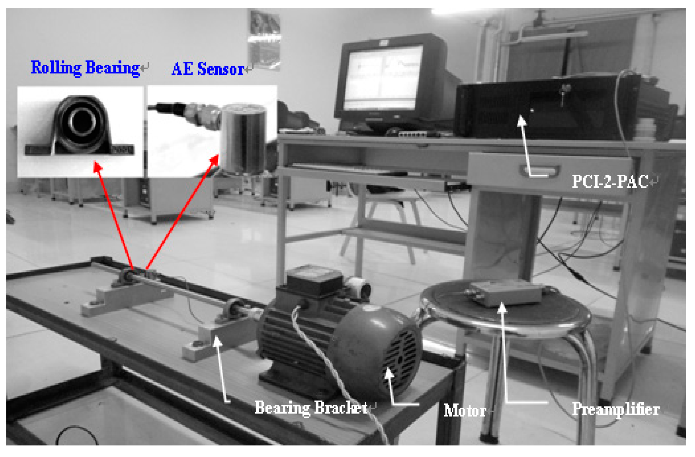
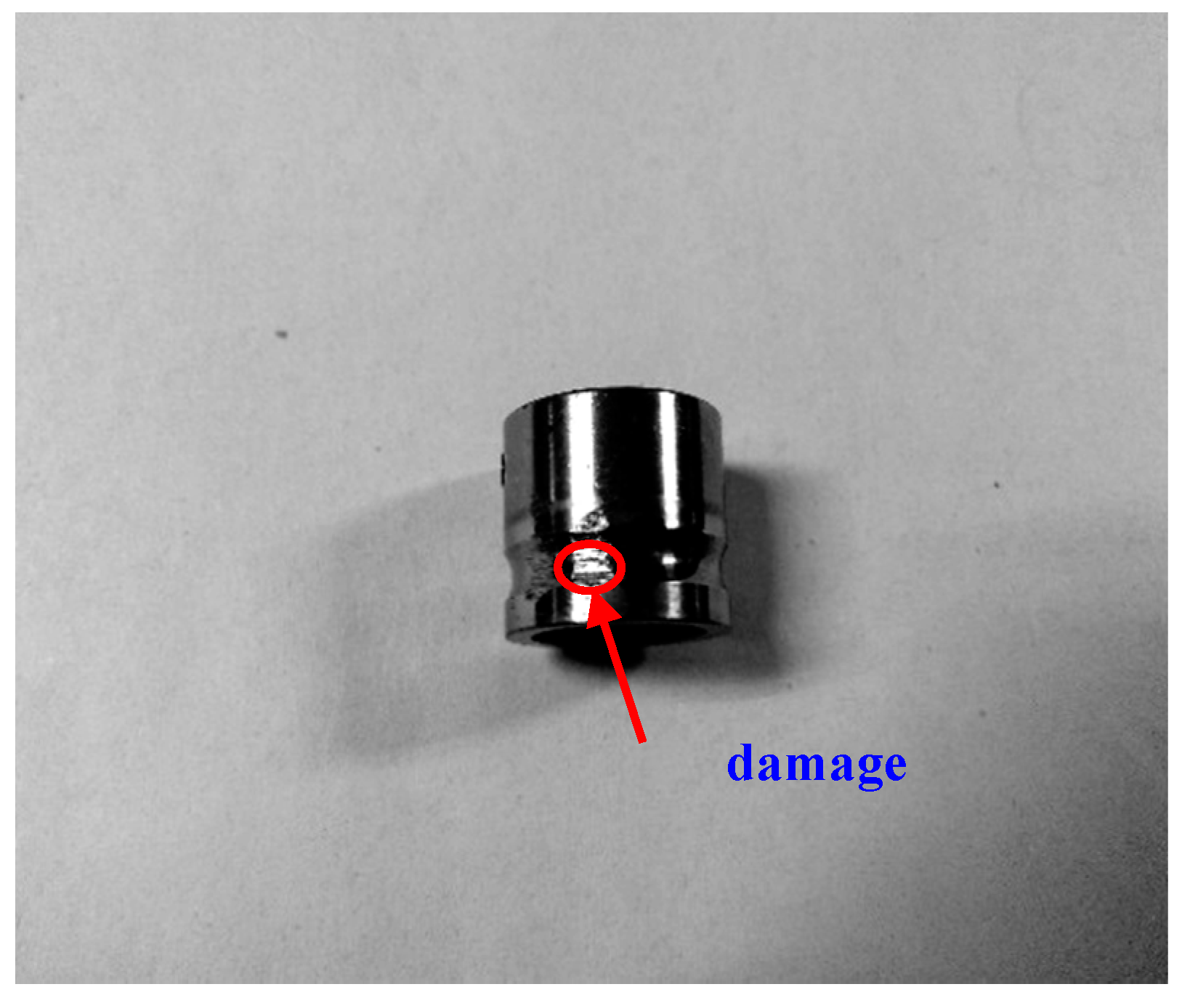
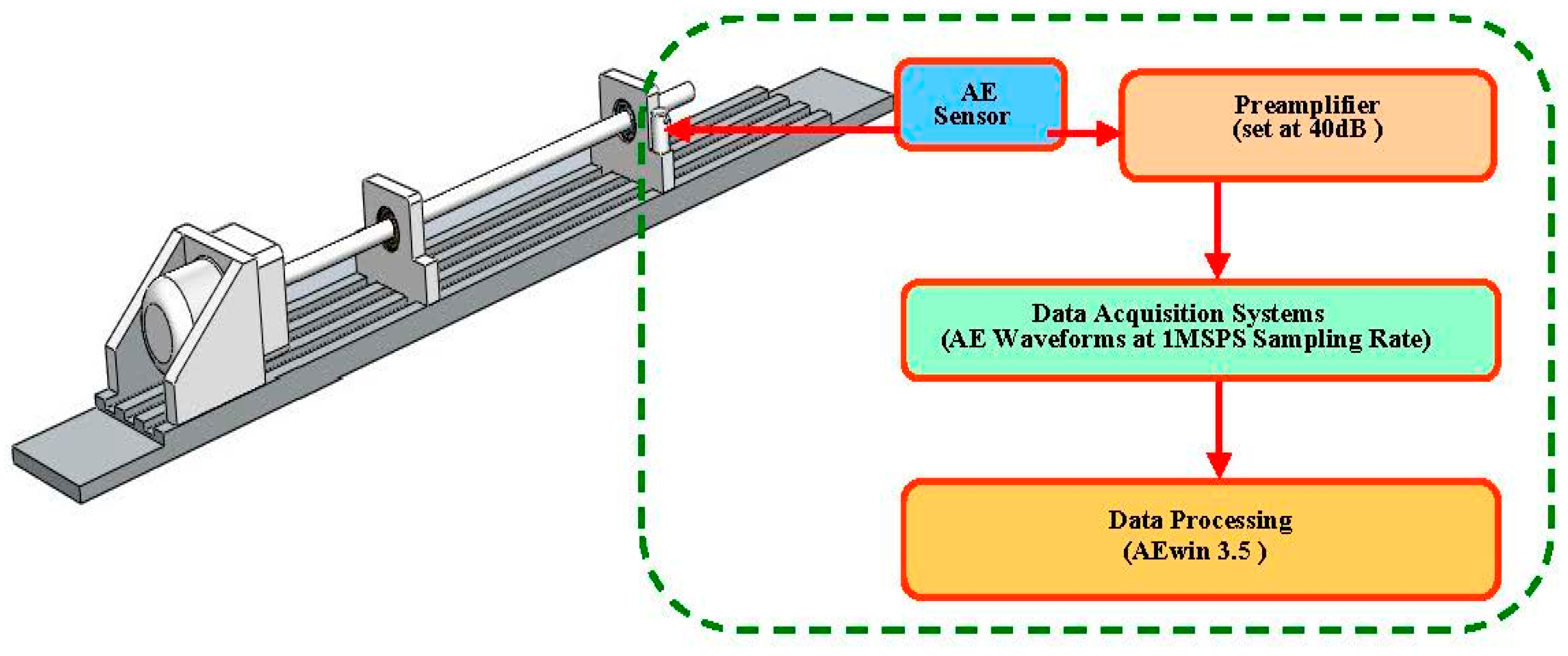
3.1. Design and Layout of Test Rig

To complete the simulation experiment, two conditions—namely, normal and damage states of the inner ring of the bearing—were tested. The rolling bearing experimental test rig is illustrated in Figure 2. The test rig consists of the motor, coupling, test bearing and support structure. The type of rolling bearing used is K001, which is produced by Chinese Nanjing haning Bearing Manufacturing Co., Ltd. The lesion area of the bearing sample is 6 mm², which is processed by electrical discharge. Physical samples are shown in Figure 3.

Figure 2. Rolling bearing experimental rig.

Figure 2. Rolling bearing experimental rig.

Figure 3. Damage fault in the inner ring of the bearing.

Figure 3. Damage fault in the inner ring of the bearing.

3.2. Instrumentation

The test instrument used in the experiment is a four-channel signal acquisition system of PCI-2-PAC produced by the American Acoustic Physics Company. The acoustic sensor is R15α, whose response frequency is 60~500 kHz and service temperature is −20~80 °C. The acoustic sensor is fixed to the stents, which are attached to the bearing by an M20 magnetic fixture. The acoustic sensor is then connected to the data acquisition system by a preamplifier (40 dB). The output impedance of the preamplifier is 50 Ω, and the working frequency is 10 KHz~2 MHz. The data acquisition systems employ AEwin 3.5 software in data acquisition and analysis. The speed of the rotating motor is 14,000 r/min, and the sampling rate is 1MSPS during the experiments. The schematic of the data acquisition process is shown in Figure 4.

Figure 4. Schematic of the data acquisition systems.

Figure 4. Schematic of the data acquisition systems.

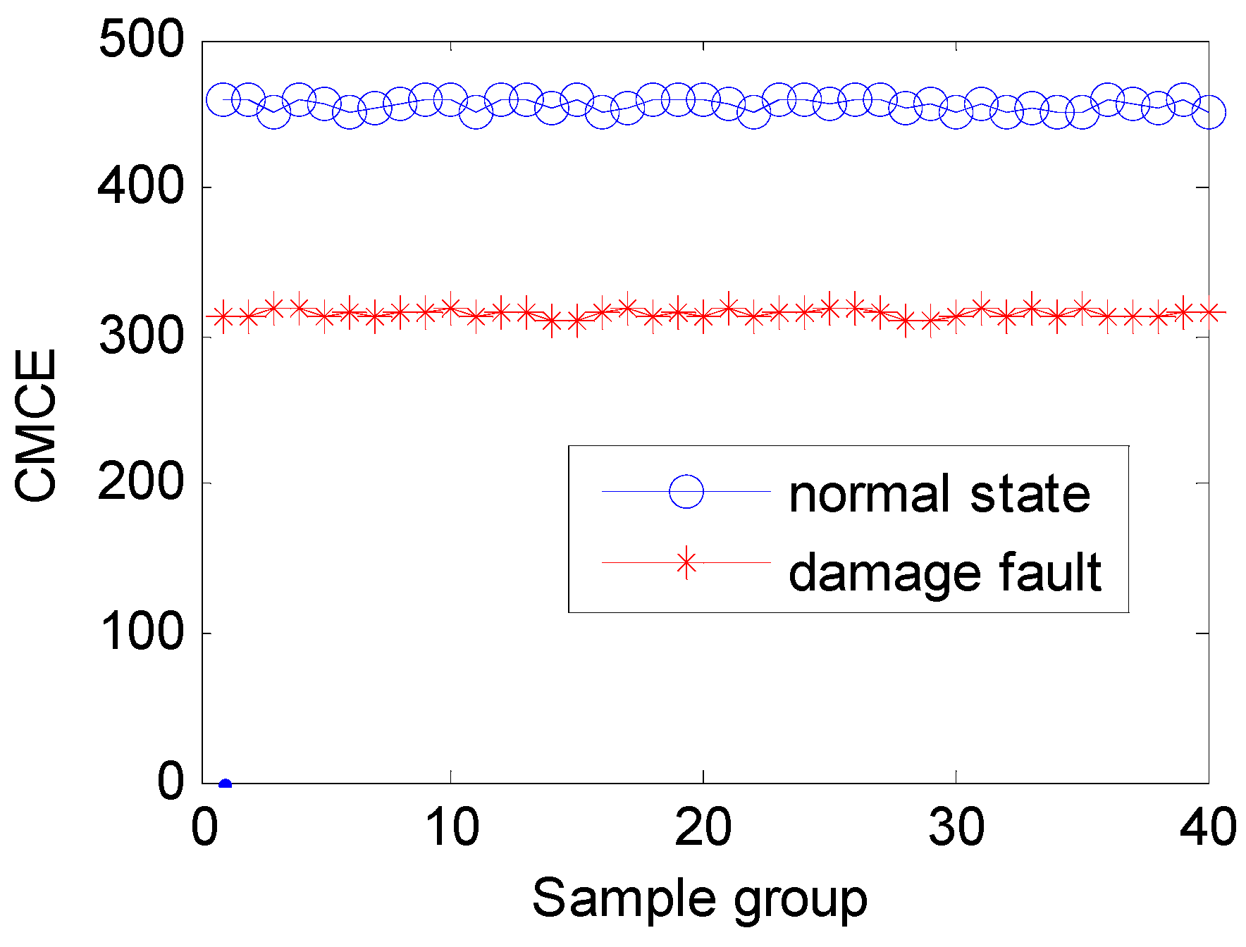
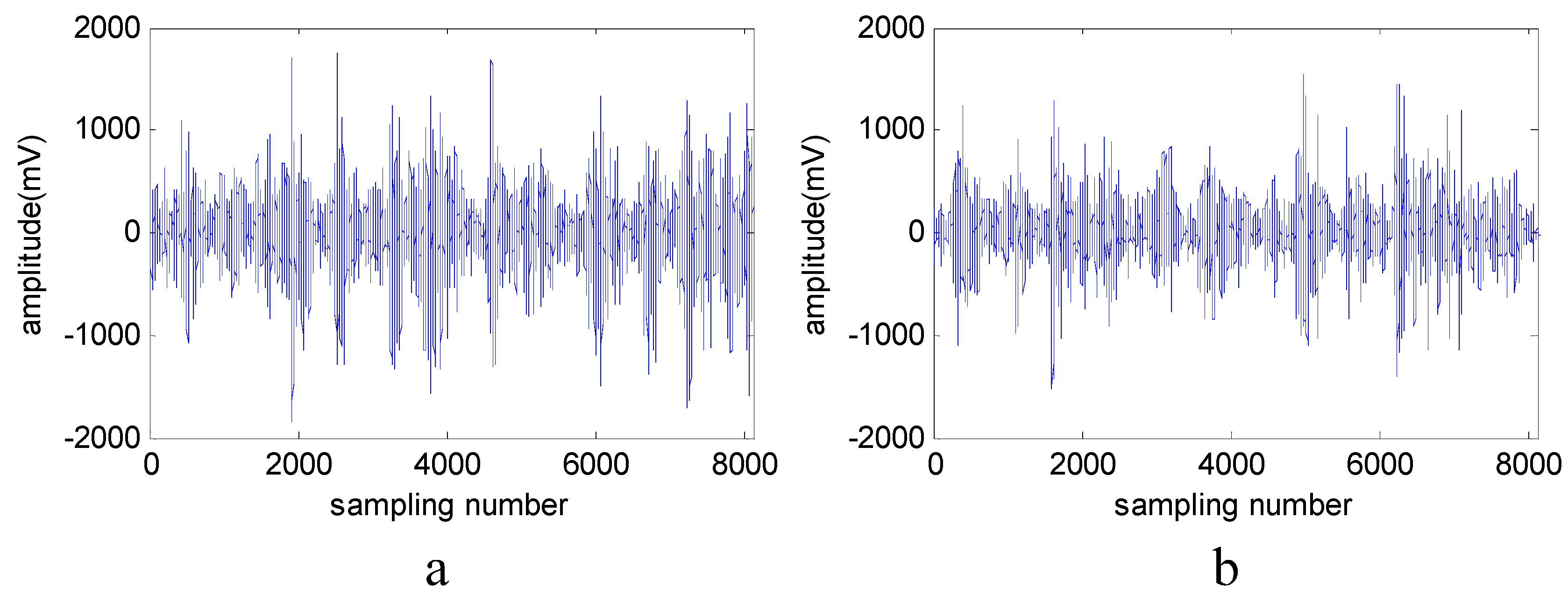
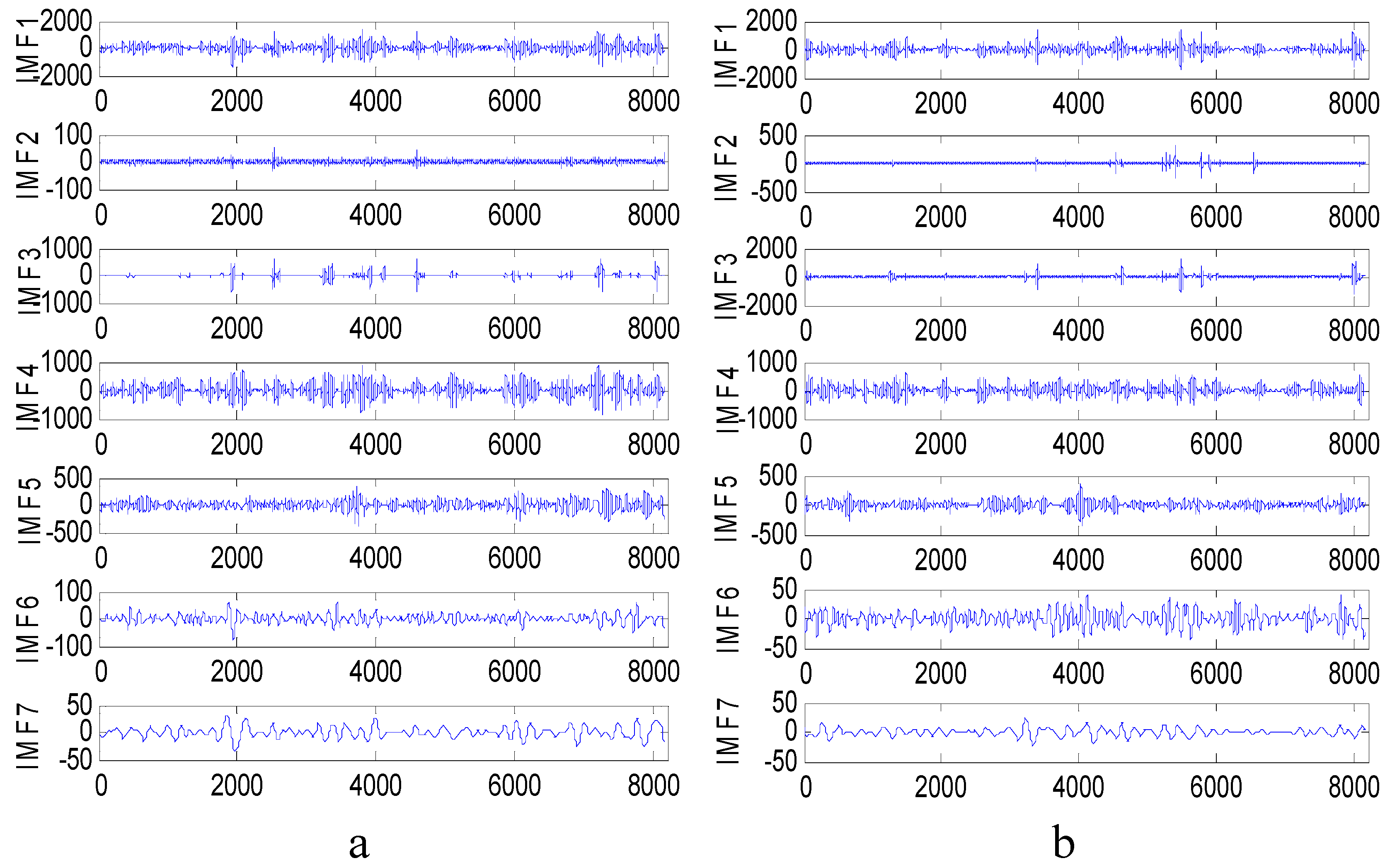
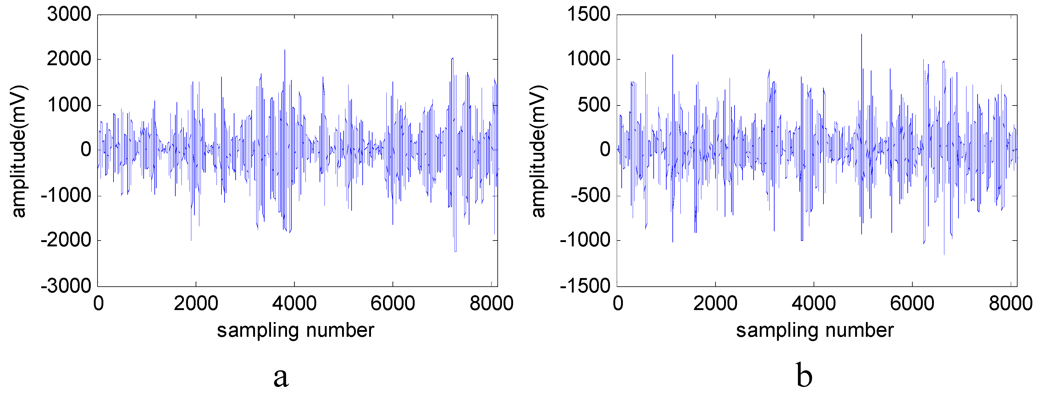
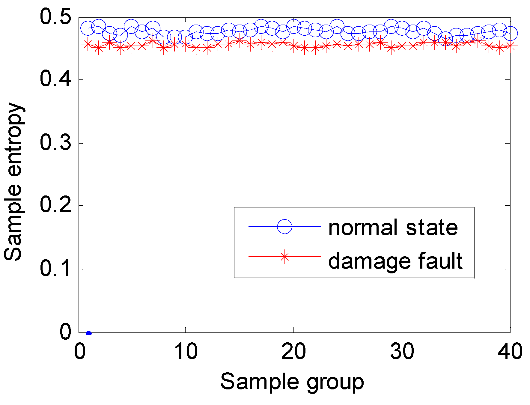
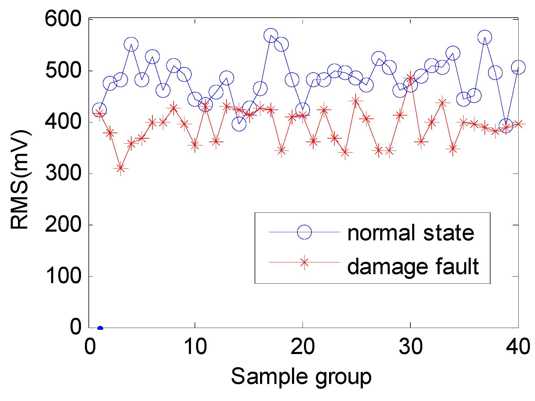
3.3. Feature Extraction of Two Kinds of Signals

The time domain waveform of the AE sensors measures the AE signals from the normal and damaged states of the inner ring of the rolling bearing, as shown in Figure 5. The decomposition of IMF1~IMF7 is achieved after the two kinds of AE signals are decomposed by the EEMD algorithm, as shown in Figure 6. The added noise amplitude value is 0.01 times of standard deviation of original signals, at the same time, The overall average time M = 200.

Figure 5. Waveforms of the two signals. (a) Normal acoustic emission (AE) signal waveform; (b) Damage AE signal waveform.

Figure 5. Waveforms of the two signals. (a) Normal acoustic emission (AE) signal waveform; (b) Damage AE signal waveform.

Figure 6. Decomposition results of the two signals. (a) The normal signal decomposition results; (b) The damage signal decomposition results.

Figure 6. Decomposition results of the two signals. (a) The normal signal decomposition results; (b) The damage signal decomposition results.

In general, the most significant information of the original signal is centralized in the first several IMF components of EEMD decomposition. The MI values between IMF1~IMF7 and the original signal under normal and damage states are calculated by the MI algorithm, as shown in Figure 7. In this figure, the abscissa mark A_i (i = 1, 2, …, 7) indicates IMF_i (i = 1, 2, …, 7) and the original signal. The normal and damage MI thresholds are calculated according to literature [19], with threshold values of 0.1452 and 0.0711, respectively. In addition, Figure 7 shows that the MI value between IMF1 and IMF4 and the original signal under normal state is higher than the threshold of 0.1452, hence, IMF1 and IMF4 are determined as sensitive IMFs. The MI value between the remaining IMFs and the original signal is lower than the threshold of 0.1452, thus, these IMFs are removed as false components. Similarly, the MI value between IMF1 and IMF4 and the original signal under damage state is higher than the threshold of 0.0711, hence, IMF1 and IMF4 are sensitive IMFs. Meanwhile, the MI values of the other IMFs are smaller than the threshold of 0.0711, and thus, these IMFs are removed as false components. In this manner, sensitive IMFs are determined under the two states. Consequently, we can obtain a summation according to sensitive IMFs. The reconstructed signals under the two states are shown in Figure 8.

Figure 7. MI value between IMF1~ IMF 7 under the two states and the original signal.

Figure 7. MI value between IMF1~ IMF 7 under the two states and the original signal.

Figure 8. Reconstruction signals. (a) The normal signal of reconstruction; (b) The damage signal of reconstruction.

Figure 8. Reconstruction signals. (a) The normal signal of reconstruction; (b) The damage signal of reconstruction.

The backward cloud generator algorithm is used to calculate the cloud model digital characteristic quantity of two kinds of reconstructed signals. The cloud model characteristic quantity of reconstruction in the damage signal is E_xa = 12.62; E_na = 317.2; and H_ea = 38.85. The cloud model characteristic quantity of reconstruction in the normal signal is E_xb = 43.62; E_nb = 443.93; and H_eb = 56.7. To conveniently observe the differences between the two kinds of cloud model, H_ea and H_eb are generally set to 0.1. The cloud model of the reconstructed signal calculated by the normal cloud generator algorithm is shown in Figure 9. As shown in the figure, the cloud models of the two kinds of reconstructed signals are obviously different. In particular, the difference between the values of cloud model characteristic entropy E_na and E_nb is significant.

Figure 9. Cloud model diagram of the reconstructed signal.

Figure 9. Cloud model diagram of the reconstructed signal.

To analyze further the distribution rules of CMCE under the two states, 40 group samples under normal and damage AE signals are selected separately. All samples should be de-noised and reconstructed by the EEMD algorithm, and the CMCE of the reconstructed signal should be calculated. The fitting curves of all CMCE values are shown in Figure 10. As shown in the figure, the distribution of CMCE under two states remains stable with the increase in sample number. Moreover, the difference between entropy values is considerable, and the effect of such difference is highly evident. Thus, CMCE can be regarded as the eigenvalue of the signals to distinguish among the different states of the bearing.

Figure 10. Fitting curves of all CMCE values under the two states.

Figure 10. Fitting curves of all CMCE values under the two states.

To compare the differences among CMCE, SampEn, and RMS, 40 sample groups of the normal and damage AE signals are selected separately. The samples should be denoised and reconstructed by the EEMD algorithm. The SampEn and RMS of the reconstructed signals should be calculated. The parameter of SampEn should be selected as follows, model dimension m = 2, threshold r = 0.2, and time series length N = 4096. The fitting curves of all SampEn and RMS values are shown in Figure 11 and Figure 12, respectively.

Figure 11. Fitting curves of all SampEn values under the two states.

Figure 11. Fitting curves of all SampEn values under the two states.

Figure 12. Fitting curves of all RMS values under the two states.

Figure 12. Fitting curves of all RMS values under the two states.

As shown in Figure 10 and Figure 11, change is relatively stable with the increasing number of sample CMCE and SampEn. However, the difference between normal and damage states of SampEn is minimal, and the distinguishing effect is not obvious. SampEn uses the unit step function, and threshold r is highly sensitive. Consequently, a sudden change occurs in SampEn, which causes the difference between the two states to decrease further. As shown in Figure 12, the RMS fluctuation of the AE signals under the two states is obvious and stability is relatively poor. Although differences occur in RMS between the normal and damage states, the distinguishing effect is poor. RMS can represent the change in signal amplitude, and thus, it is easily disturbed by the environment, has poor anti-noise capability, and fails to solve the signal uncertainty problem. Moreover, obvious fluctuations easily appear with the increase in sample number.

The CMCE and SampEn of the reconstructed signal are set as the eigenvalue. Fault diagnosis is performed with K-nearest neighbor (KNN) classification algorithm and support vector machine (SVM) algorithm [20,21,22]. One hundred and twenty groups of samples are selected from CMCE and SampEn samples, respectively, among which, 80 groups are for training and 40 groups are for testing. Setting K = 3 in K-nearest neighbor (KNN) classification algorithm, the penalty factor C = 150, σ = 1 in support vector machine (SVM) algorithm, the experimental results are shown in Table 1, which show that the diagnostic performances of KNN and SVM are both good under EEMD–CMCE. Also, this shows that the proposed EEMD–CMCE method is a better Feature Extraction method than the EEMD–SampEn method.

Table 1. Comparison of fault diagnosis results.

	Accuracy %
Method	KNN	SVM
EEMD–CMCE	96.2	97.5
EEMD–SampEn	83.4	88.7

Table 1. Comparison of fault diagnosis results.

	Accuracy %
Method	KNN	SVM
EEMD–CMCE	96.2	97.5
EEMD–SampEn	83.4	88.7

4. Conclusions

This study proposes a feature extraction method based on the EEMD and CMCE of rolling bearing fault signal. The EEMD algorithm is used in signal decomposition. Sensitive IMFs are then selected to reconstruct signals using the MI method, which finally eliminates noise. CMCE is used as the eigenvalue of the reconstructed signal to overcome the disadvantages of traditional entropy. According to the analysis of the AE signals from a rolling bearing under normal and damage states, the experimental results verify that the index, as bearing fault characteristics, is effective and superior.

References

- Li, B.Y.; Feng, J.L.; Dai, G.; Li, W. Progress in the study of acoustic emission for evaluation of pitting corrosion in metal. Tech. Acoust. 2005, 24, 170–172. [Google Scholar]
- Elforjani, M.; Mba, D. Monitoring the Onset and Propagation of Natural Degradation Process in a Slow Speed Rolling Element Bearing With Acoustic Emission. J. Vib. Acoust. 2008, 130, 1257–1261. [Google Scholar] [CrossRef]
- Al-Ghamdi, A.M.; Cole, P.; Such, R.; Mba, D. Estimation of bearing defect size with acoustic emission. Insight Non-Destr. Test. Cond. Monit. 2004, 46, 758–761. [Google Scholar] [CrossRef]
- Beck, P.; Bradshaw, T.P.; Lark, R.J.; Holford, K.M. A quantitative study of the relationship between concrete crack parameters and acoustic emission energy released during failure. Key Eng. Mater. 2003, 245–246, 461–466. [Google Scholar] [CrossRef]
- Kilundu, B.; Chiementin, X.; Duez, J.; Mba, D. Cyclostationarity of acoustic emissions (AE) for monitoring bearing defects. Mech. Syst. Signal Process. 2011, 25, 2061–2072. [Google Scholar] [CrossRef]
- Xu, F.; Liu, Y. Feature Extraction and Classification Method of Acoustic Emission Signals Generated from Plywood Damage Based on EMD-SVD. J. Basic Sci. Eng. 2014, 22, 1238–1247. [Google Scholar]
- Wu, Z.H.; Huang, N.E. Ensemble empirical mode decomposition: A noise assisted data analysis method. Adv. Adapt. Data Anal. 2009, 1, 1–41. [Google Scholar] [CrossRef]
- Yan, R.; Gao, R.X. Approximate entropy as a diagnostic tool for machine health monitoring. Mech. Syst. Signal Process. 2007, 21, 824–839. [Google Scholar] [CrossRef]
- Su, W.; Wang, F.; Zhu, H.; Guo, Z.; Zhang, Z.; Zhang, H. Feature extraction of rolling element bearing fault using wavelet packet sample entropy. J. Vib. Meas. Diagn. 2011, 31, 162–166. [Google Scholar]
- Li, D.Y.; Liu, C.Y.; Gan, W.Y. A new cognitive model: Cloud model. Int. J. Intell. Syst. 2009, 24, 357–375. [Google Scholar] [CrossRef]
- Li, H.L.; Guo, C.H. Piecewise aggregate approximation method based on cloud model for time series. Control Decis. 2011, 26, 1525–1529. [Google Scholar]
- Yu, N.H.; Li, L.F.; Wang, L. Abnormal Detection for Harmonic Currents Based on Cloud Model (In Chinese). CSEE Proc. 2014, 34, 4395–4401. [Google Scholar]
- Liu, H.J.; Liu, Z.; Jiang, W.L. A Method for Emitter Recognition Based on Cloud Model. J. Electron. Inf. Technol. 2009, 31, 2079–2083. [Google Scholar]
- Xu, H.J.; Wang, Z.Y.; Su, H.Y. Dissolved gas analysis based feedback cloud entropy model for power transformer fault diagnosis. Power Syst. Prot. Control 2013, 41, 115–119. [Google Scholar]
- Dang, Q.; Luo, J.W.; Wang, D. Research of anomaly detection algorithm based on cloud theory. Appl. Res. Comput. 2009, 26, 3724–3726. [Google Scholar]
- Zhang, J.; Yan, R.; Gao, R.X. Performance Enhancement of Ensemble Empirical Mode Decomposition. Mech. Syst. Signal Process. 2010, 2, 1018–1026. [Google Scholar] [CrossRef]
- Shen, Y.; Wang, L.; Zhao, Z. Fault diagnosis for rolling bearing of wind turbine based on improved HHT. Meas. Control Technol. 2013, 32, 40–44. [Google Scholar]
- Li, D.Y.; Du, Y. Artificial Intelligence with Uncertainty; National Defense Industry Press: Beijing, China, 2005; pp. 143–185. [Google Scholar]
- Albert, A.-P.; Nii, A.-O. A criterion for selecting relevant intrinsic mode functions in empirical mode decomposition. Adv. Adapt. Data Anal. 2011, 2. [Google Scholar] [CrossRef]
- Yuan, S.; Chu, F. Support vector machines and its application in machine fault diagnosis. J. Vib. Shock 2007, 26, 29–35. [Google Scholar]
- Salzberg, S.L. On comparing classifiers: Pitfalls to avoid and a recommended approach. Data Min. Knowl. Discov. 1997, 1, 317–328. [Google Scholar] [CrossRef]
- Zhu, B.; Yang, J.; Lv, W.; Chen, L.; Ma, Y.; Yao, W.; Zhang, Y. Ground-based visible cloud image classification methodbased on KNN algorithm. J. Appl. Meteorol. Sci. 2012, 23, 721–728. [Google Scholar]
© 2015 by the authors; licensee MDPI, Basel, Switzerland. This article is an open access article distributed under the terms and conditions of the Creative Commons Attribution license (http://creativecommons.org/licenses/by/4.0/).
Share and Cite
Han, L.; Li, C.; Liu, H. Feature Extraction Method of Rolling Bearing Fault Signal Based on EEMD and Cloud Model Characteristic Entropy. Entropy 2015, 17, 6683-6697. https://doi.org/10.3390/e17106683
Han L, Li C, Liu H. Feature Extraction Method of Rolling Bearing Fault Signal Based on EEMD and Cloud Model Characteristic Entropy. Entropy. 2015; 17(10):6683-6697. https://doi.org/10.3390/e17106683
Chicago/Turabian StyleHan, Long, Chengwei Li, and Hongchen Liu. 2015. "Feature Extraction Method of Rolling Bearing Fault Signal Based on EEMD and Cloud Model Characteristic Entropy" Entropy 17, no. 10: 6683-6697. https://doi.org/10.3390/e17106683
APA StyleHan, L., Li, C., & Liu, H. (2015). Feature Extraction Method of Rolling Bearing Fault Signal Based on EEMD and Cloud Model Characteristic Entropy. Entropy, 17(10), 6683-6697. https://doi.org/10.3390/e17106683